1. Introduction
Being able to make a profit consistently in Forex trading continues to remain a challenging endeavour, especially given the numerous factors that can influence price movements [
1]. To be successful, traders have to not only predict the market signals correctly, but also perform risk management to mitigate their losses in the event the market moves against them [
2]. As such, there has been increasing interest in developing automated system-driven solutions to assist traders in making informed decisions on the course of action they should take given the circumstances [
3]. However, these solutions tend to be rule-based or require the inputs of subject matter experts (SMEs) to develop the knowledge database for the system [
4]. This approach would negatively impact the performance of the system in the long run given the dynamic nature of the market, as well as making it cumbersome to update [
5].
Most recently, newer innovations have introduced more intelligent approaches through the use of advanced technologies, such as ML algorithms [
6]. Unlike the traditional rule-based approach, machine learning is able to analyze the Forex data and extract useful information from it to help traders make a decision [
7]. Given the explosion of data and how it is becoming more readily available nowadays, this has been a game-changer in the field of Forex trading with its fast-paced automated trading since it requires little human intervention and provides accurate analysis, forecasting, and timely execution of the trades [
8].
This study proposes a complete end-to-end system solution, coined as AlgoML, that incorporates both trade decisions as well as a risk and cash management strategy. The system is able to automatically extract data for an identified Forex pair, predict the expected market signal for the next day and execute the most optimal trade decided by the integrated risk and cash management strategy. The system incorporates several SOTA reinforcement learning, supervised learning, and optimized conventional strategies into a collective ensemble model to obtain the predicted market signal. The ensemble model gathers the output predicted signal of each strategy to give an overall final prediction. The risk and cash management strategy within the system helps to mitigate risk during the trade execution phase. In addition, the system is designed such that it makes it easier to train and back test strategies to observe the performance before actual deployment.
The paper is structured as follows:
Section 2 explores related works on prediction based models for the Forex market.
Section 3 presents the high-level architecture of the system and its individual modules.
Section 4 elaborates on the ML model designs used in the system.
Section 5 provides the results on the performance of the system.
2. Related Works
Over the past decade, there have been a number of works in the literature proposing various prediction-based models for trading in the Forex market. One of the most popular time-series forecasting models was Box and Jenkins’ auto-regressive integrated moving average (ARIMA) [
3], which is still explored by other researchers for Forex prediction [
9,
10]. However, it is noted that ARIMA is a general univariate model and it is developed based on the assumption that the time series being forecasted are linear and stationary [
11].
With the advancement of machine learning, most of the research works have been focused on the use machine learning techniques to develop the prediction models. One such area is the use of supervised machine learning models. Kamruzzaman et al. investigated artificial neural networks (ANNs)-based prediction modeling of foreign currency rates and made a comparison with the best known ARIMA model. It was discoverd that the ANN model outperformed the ARIMA model [
12]. Thu et al. implemented a support vector machine (SVM) model with actual Forex transactions, and outlined the advantages of the use of SVM compared to transactions done without the use of SVM [
13]. Decision trees (DT) have also seen some usage in Forex prediction models. Juszczuk et al. created a model that can generate datasets from real-world FOREX market data [
14]. The data are transformed into a decision table with three decision classes (BUY, SELL or WAIT). There are also research works using an ensemble model rather than relying on single individual models for Forex prediction. Nti et al. constructed 25 different ensembled regressors and classifiers using DTs, SVMs and NNs. They evaluated their ensembled models over data from various stock exchanges and showed that stacking and blending ensemble techniques offer higher prediction accuracy of (90–100%) and (85.7–100%) respectively, compared with that of bagging (53–97.78%) and boosting (52.7–96.32%). The root mean square error (RMSE) recorded by stacking (0.0001–0.001) and blending (0.002–0.01) was also lower than to that of bagging (0.01–0.11) and boosting (0.01–0.443) [
15].
Apart from supervised machine learning models, another area of machine learning technique that is employed for Forex prediciton is the use of Deep Learning models. Examples of such models include long short-term memory (LSTM) and convolutional neural networks (CNNs). Qi et al. conducted a comparative study of several deep learning models, which included long short-term memory (LSTM), bidirectional long short-term memory (BiLSTM) and gated recurrent unit (GRU) against a simple recurrent neural network (RNN) baseline model [
16]. They concluded that their LSTM and GRU models outperformed the baseline RNN model for EUR/GBP, AUD/USD and CAD/CHF currency pairs. They also reported that their models outperformed those proposed by Zeng and Khushi [
17] in terms of RMSE, achieving a value of 0.006 × 10
as compared to 1.65 × 10
for the latter.
Some research works have attempted a hybrid approach by combining multiple deep learning models together. Islam et al. introduced the use of a hybrid GRU-LSTM model. They have tested their proposed model on 10-mins and 30-mins timeframes and evaluated the performance based on MSE, RMSE, MAE and R
2 score. They reported that the hybrid model outperforms the standalone LSTM and GRU model based on the performance metrics used [
18].
Reinforcement learning (RL) is another area of interest that has been tapped for Forex prediction. It involves training an agent to interact with the environment by sequentially receiving states and rewards from the environment and taking actions to reach better rewards. In the case of Forex trading, the reward function can be based on maximising prediction accuracy or profit. Carapuço et al. developed a neural network with three hidden layers of ReLU neurons are trained as RL agents under the Q-learning algorithm by a novel simulated market environment framework, which includes new state and reward signals. They tested their model on the EUR/USD market from 2010 to 2017, and the the system yielded an average total profit of 114.0 ± 19.6% for an yearly average of 16.3 ± 2.8% over 10 tests with varying initial conditions [
19]. Other works have been done in deep reinforcement learning (DRL) techniques, which combines machine learning and reinforcement learning. Thibaut and Ernst presented a deep reinforcement learning (DRL) approach inspired by the popular Deep Q-Network (DQN) algorithm [
20]. Yuan et al. found that proximal policy optimization (PPO) is the most stable algorithm to achieve high risk-adjusted returns, while (DQN) and soft actor critic (SAC) can beat the market in terms of Sharp ratio [
21]. Rundo proposed an algorithm that uses a deep learning LSTM network with reinforcement learning layer for high-frequency trading in the Forex market. The model was reported to achieve an accuracy of 85%. The algorithm was further validated on the EUR/USD market, achieving a return of investment of 98.23% and reduced drawdown of 15.97% [
22].
Although there has been extensive research work done in trying to develop prediction models for Forex prediction, especially in the use of machine learning techniques, it is noted that the results are heavily focused on accuracy metrics. As such, there is a lack of profitability results, which is important to consider as well since the main goal of Forex trading is to generate profits. However, generating profits is not just dependent on the model getting most of the predictions right. In a real-world trading context, there are many other factors that come into play that can significantly impact profit such as transaction costs [
23,
24], which can quickly erode profits if many trades are conducted in a short time span. Furthermore, there is little to no research work conducted for a complete end-to-end system solution that includes features such as comprehensive back testing and optimization, which is important for actual deployment on the real world Forex trading environment. Hence, this study aims to address the shortcomings identified in this field through a proposed complete end-to-end system solution for Forex trading.
3. Methods
3.1. Overall Architecture
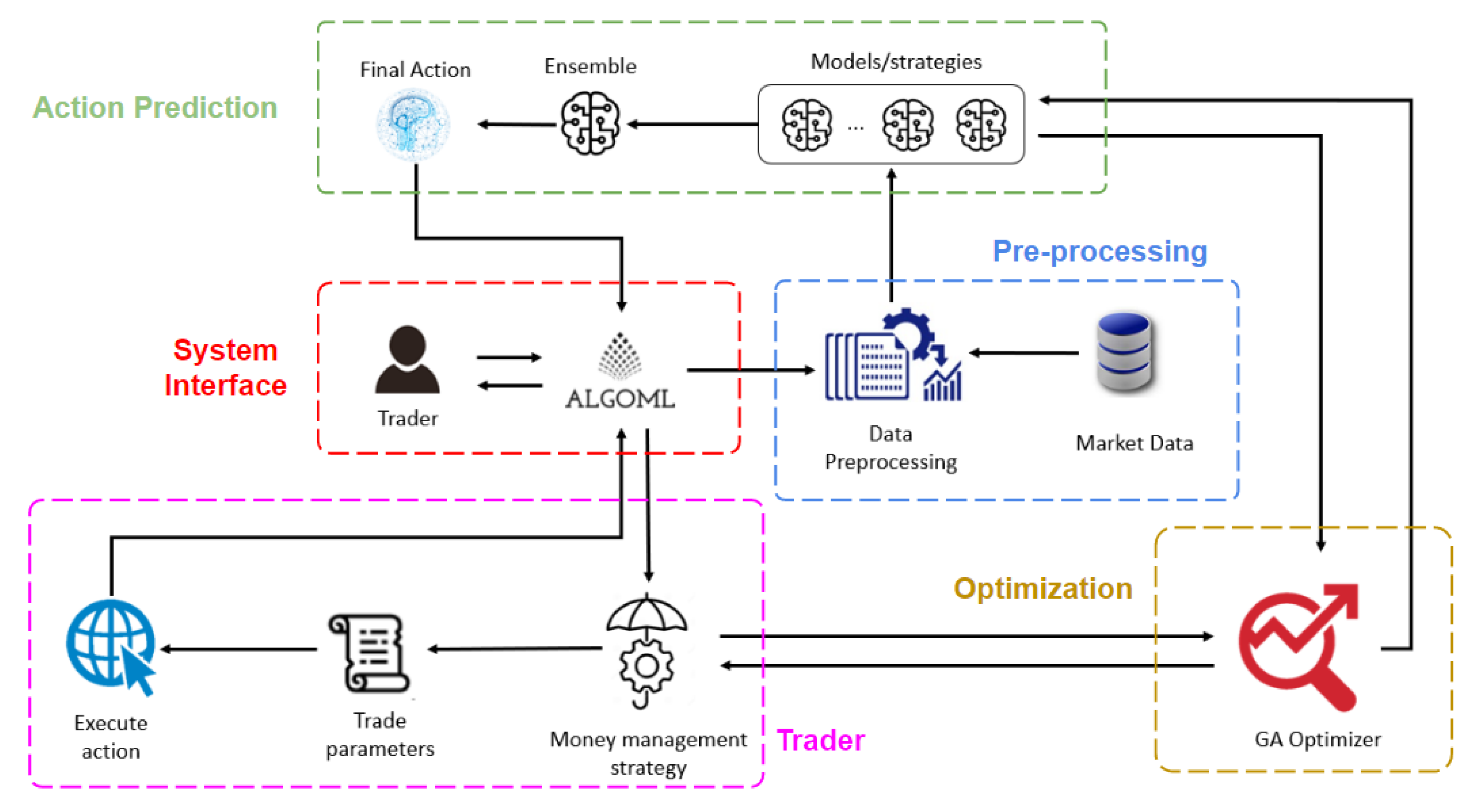
The high level architecture of the proposed system is illustrated in
Figure 1, and consists of the following 5 main modules:
System Interface module: UI interface that traders can use to communicate with AlgoML to obtain trade action recommendation and execute trades through broker websites.
Pre-processing module: includes the extract, load and transform pipeline together with data cleaning, feature extraction and feature engineering
Action Predictor module: gives a final predicted buy/sell action output
Trader module: simulator environment to replicate market trading and execute orders based on model predictions. Also performs actual trade through broker websites
Optimizer module: optimizes parameters for strategies to improve system profitability
With reference to
Figure 1, the general process flow of the system starts out at the System Interface module. Traders will use the UI to ask AlgoML to provide a recommended action for their desired Forex pair. Upon receiving the request, the system proceeds to the Pre-processing module, where market data is harvested through broker websites and processed accordingly. The processed data is then passed into the Action Predictor module, specifically into the various models/strategies included within it. Each model/strategy takes in the processed data and outputs their predicted action to take. The predicted action from each model/strategy is then collected into the ensemble model to obtain a single final predicted action. The predicted action to take will then be reflected to the user via the System Interface UI. Here, the user can choose to instruct AlgoML to execute the predicted action on their behalf. If so, the system will proceed to the Trader module, which takes in the predicted action signal and uses an included money management strategy to execute the most optimal course of action to take. The result of the actual action taken by the Trader module will be reflected back to the user through the UI. The Optimization module of the system helps to optimize parameters for strategies within the system such as the money management strategy in the Trader module, and those used in the Action Predictor module. More details about how each module functions is explained in
Section 3.2,
Section 3.3,
Section 3.4,
Section 3.5 and
Section 3.6 below.
3.2. System Interface Module
The System Interface module consists of a front-end UI built using Python’s tkinter package. Using the UI, traders can select the Forex pair that they wish to trade using AlgoML. After selecting the desired Forex pair, traders will command AlgoML to extract the most update-to-date OHLCV data available for that Forex pair through broker websites. After that, traders can request AlgoML to make a prediction of whether they should “BUY” or “SELL” based on the data available at hand, which will be reflected on the UI once the prediction is completed. If traders wish for AlgoML to execute the trade on their behalf, it can be done so through the UI.
3.3. Pre-Processing Module
3.3.1. Data Preparation
The Pre-processing module first performs extract, transform and load (ETL) to obtain the raw data of the identified Forex pair (EUR/USD) through the broker websites. Data that are extracted come in the form of “Open, High, Low, Close and Volume” (OHLCV). In total, 8 years’ worth of daily OHLCV data from January 2010 to December 2018 were selected as training data set, while test data were from January 2020 to December 2020. Data from year 2019 were intended to leave as a gap between training and test data set to prevent data leakage due to some technical indicators requiring lookback, for example moving average.
Labels are generated to train the models. Since the expected market signal output from the system is either a “BUY” or “SELL” signal, the labels are denoted as “1” for “BUY” signals and “−1” for “SELL” signals. The labels are generated by taking the difference in ‘Close’ price between the next day (
t + 1) and current day (t) as shown in (1) and (2). If the difference is positive, then the label is “1” since the close price is expected to go up the next day. Otherwise, the label is “−1” since the close price is expected to go down the next day.
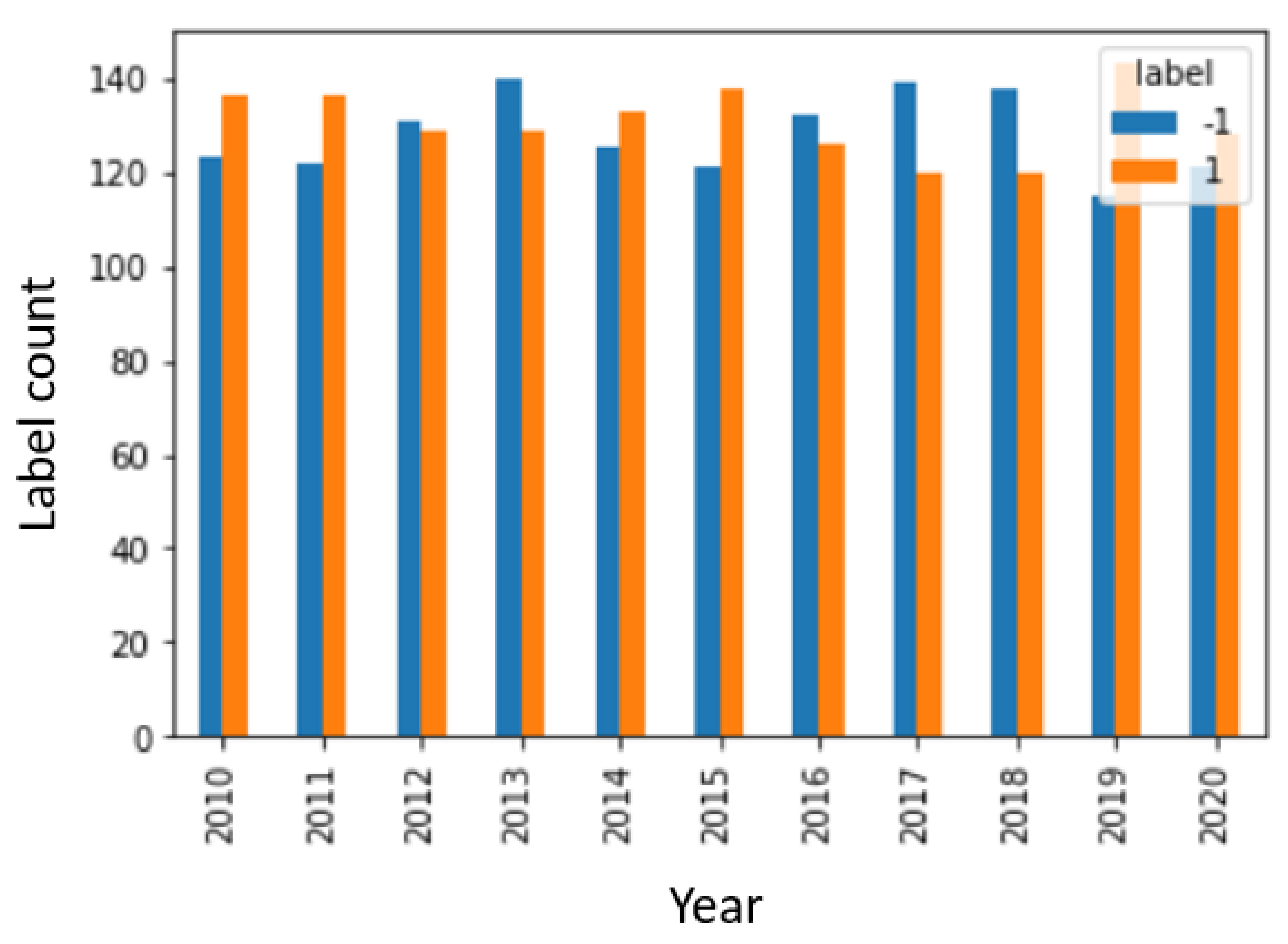
After generating the labels, it is important to check for class imbalance within the data. This is to prevent biased performance of the trained model towards a certain set of labels [
25]. The presence of class imbalance can be observed by checking the labels distribution for each year as shown in
Figure 2. A good class distribution would have a relatively similar number of labels for each year and overall total for the entire time range as well, which can be observed from the graph. As such, class imbalance is not expected to be major factor negatively affecting the performance of the trained supervised models.
3.3.2. Eliminating Trend and Seasonality in Data
Times series data is different from independent and identically distributed (IID) data. The conventional preprocessing methods cannot be applied directly to this data. Furthermore, financial price data follows a stochastic process which adds a further level of complexity. As such, it would be extremely difficult to model or forecast the data [
26,
27]. Hence, when dealing with time-series data, it is recommended to make the data stationary before passing it into the model for training and testing. Stationary data is where the mean, variance and autocorrelation structure do not change over time, which means that there should be no clear trend observed within the data [
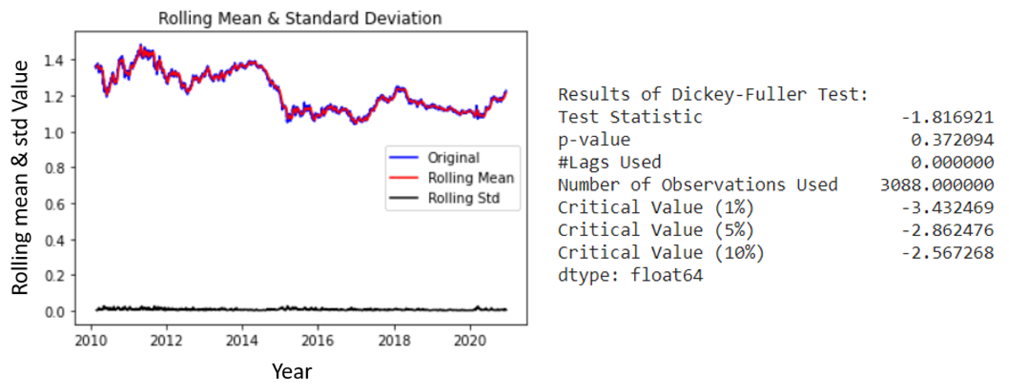
28]. The motive behind making data stationary is that ML models learn based on particular patterns. Due to regime changes or external factors, the market changes and so do the patterns in the data. As such, predictive results are going to be worse, as the ML model is unable to generalize well to this change in pattern. To test whether a time-series is truly stationary or not, the augmented Dickey–Fuller (ADF) test is utilized [
29]. The main objective of the test is to reject the null hypothesis that the data is nonstationary. If the null hypothesis can be rejected, it means that the data is stationary. The test consists of a Test Statistic and some Critical Values for different confidence levels. If the ‘Test Statistic’ is less than the ‘Critical Value’, then the null hypothesis can be rejected. When applied to the raw OHLCV data, the results as seen in
Figure 3 show that the data is indeed nonstationary.
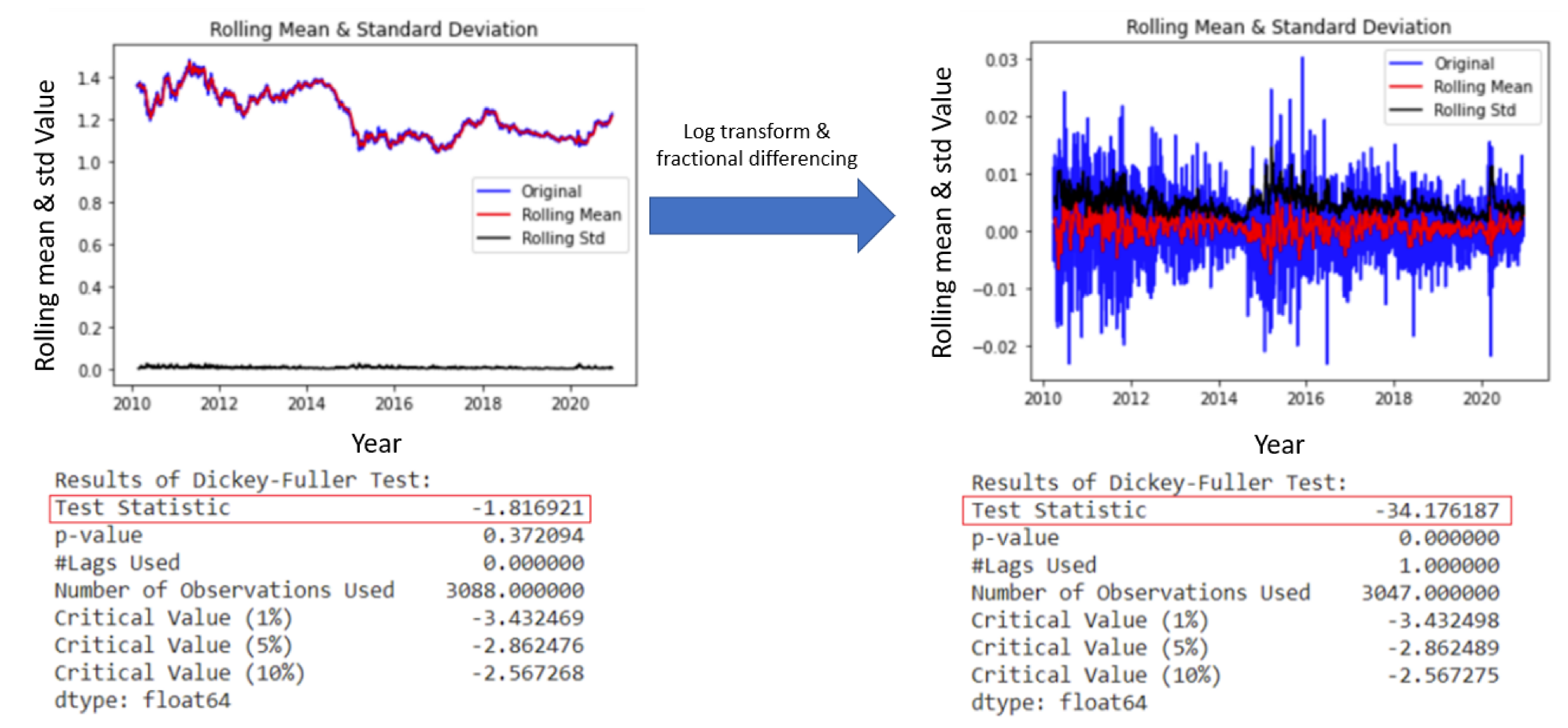
To make the OHLCV data stationary, a combination of log transformation and fractional differencing is used. The reason for this is that it was discovered that solely applying a log transform does not make the data stationary based on the ADF test; thus, fractional differencing was also used in conjunction to make the data stationary. Log transform attempts to reduce trend and seasonality by penalizing higher values more than smaller values. Fractional differencing is chosen instead of integer differencing because the latter unnecessarily removes too much memory to achieve stationarity, which could affect the predictive performance of the ML models. Thus, fractional differencing helps to achieve stationarity while maintaining the maximum amount of memory compared to integer differencing. The formula for fractional differencing [
30] is outlined in (
3).
where
denotes fractional differencing of order
d.
Since the differencing order is fractional, each of the lags has a weight, and they converge to zero in absolute value (faster convergence towards zero happens in higher orders of differencing), a cutoff value is required for the absolute value of the coefficients such that the series is not theoretically infinite. Larger time series would allow smaller cutoff values in order to preserve more memory, it ends up being a trade-off between memory conservation and computational efficiency. For this study, a differencing order of 0.8 is used, which will cut off around 2% of data entries from the raw nonstationary dataset. This is to establish a good balance between making the data stationary and preserving as much memory as possible. After applying both log transform and fractional differencing, the results of the ADF test as seen in
Figure 4 indicates that the the null hypothesis of the test can be rejected and the data is now deemed to be stationary.
3.3.3. Feature Engineering
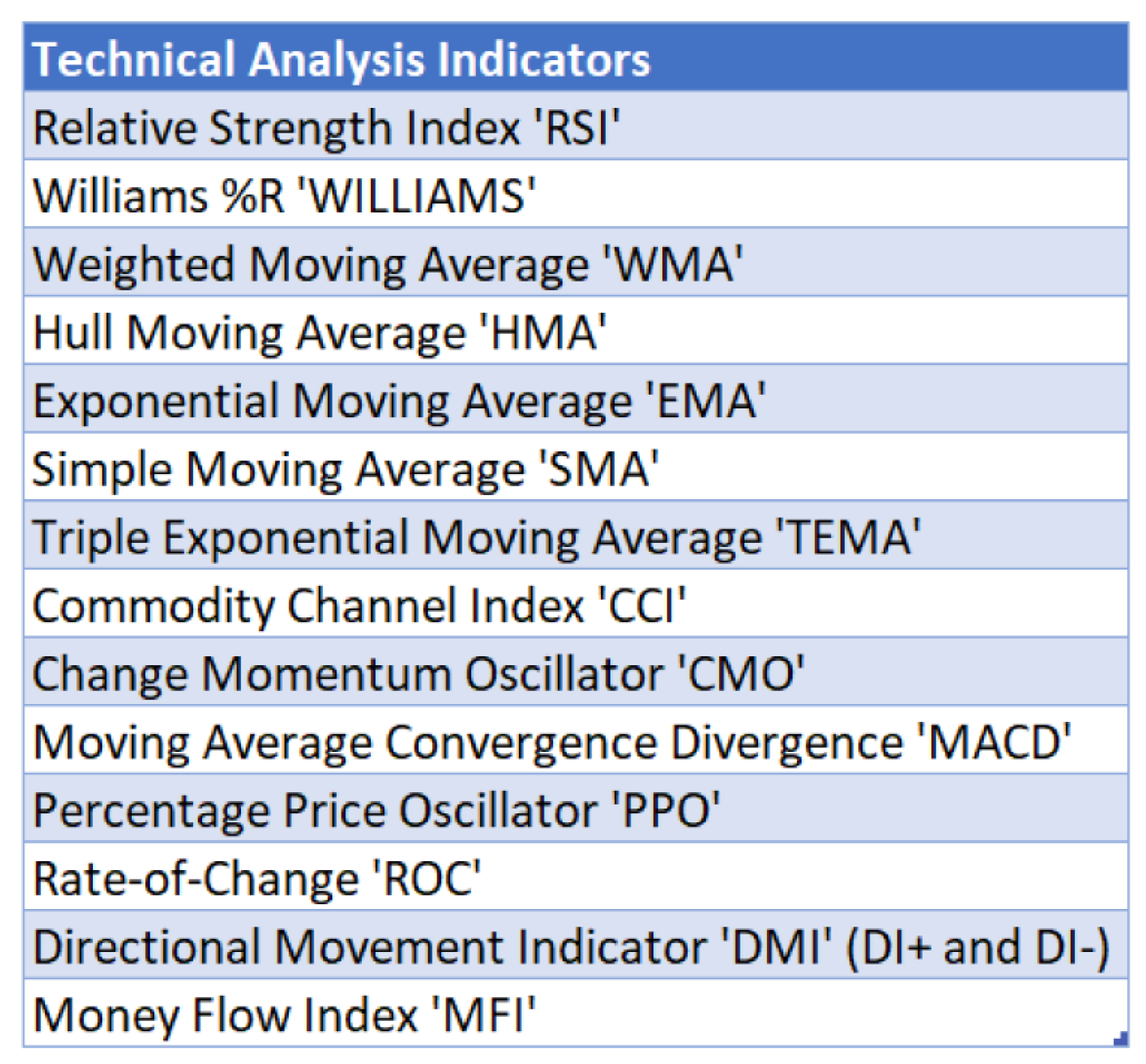
In real world trading, traders do not just depend on analyzing OHLCV signals to predict market movement. Instead, they also employ the use of technical indicators, which are heuristic or pattern-based signals produced by the price or volume data. Examples of commonly used technical indicators include moving average (MA), Bollinger bands (BB) and Heikin Ashi candles. Some notable technical indicators that are used to train the ML models in the system are seen in
Figure 5, which have been used in other research works for Forex trading as well [
31,
32]. The chosen technical indicators are mostly oscillators and trend-based financial time-series filters which are used by [
32]. In those studies, different intervals are used for the technical indicators (3, 7, 14 and 20 days), which are commonly preferred by short-to-medium-term traders. The conclusion drawn from [
33] reveals that using long-horizon forecasts potentially contributes to negative prediction results and short-term results in better prediction. This is based on the fact that out of the 39 studies, 27 papers used both middle-term and short-term predictions. The technical indicators are generated using Python packages finta [
34] and pandas-ta [
35].
The technical indicators selected from
Figure 5 along with the Open, High, Low, Close, Volume are being normalized using MinMax scaler from scikit-learn preprocessing library. A total of 19 parameters were used to train the deep learning models.
3.4. Action Predictor Module
The Action Predictor module uses an ensemble technique, where results from several ML models are combined together to give a final predicted buy/sell action output. As compared to single-model based predictions, ensemble models have the advantage to potentially reduce the variance of predictions and reduce generalization error, resulting in better performance than the former approach [
25]. This makes it applicable for the Forex markets as they tend to be very volatile, which makes predictions very prone to high-variance errors. Various works have incorporated ensemble methods to achieve state-of-the-art performance [
36,
37]. Other studies involved in stock market price prediction have reported that ensemble models produced a higher accuracy prediction as compared to single models [
38,
39].
The three key criteria while designing the ensemble were the choice of base learners, the combination techniques used to aggregate the predictions and the quantum of classifiers to be ensembled. The Action Predictor module consists of two main parts: the base learner module, which includes the various ML models, and the Ensemble module, to combine the predictions and output a single final predicted action.
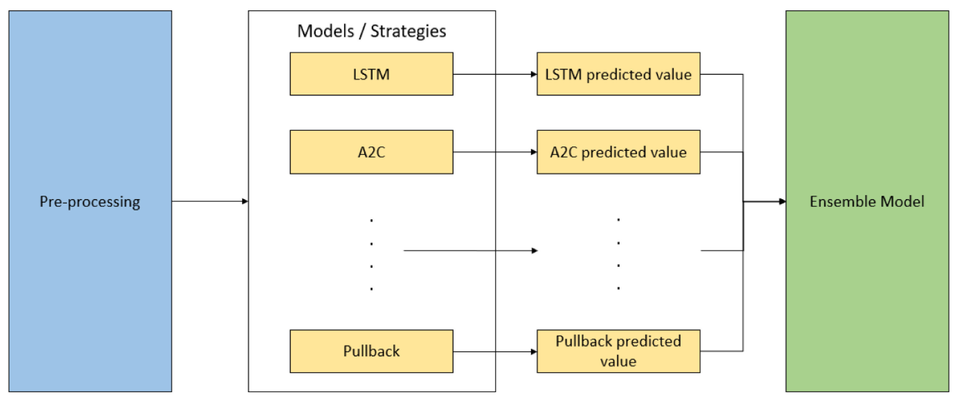
With reference to
Figure 6, the base learner module consists of various machine learning classifier models. All models/strategies will receive the preprocessed input from the preprocessing module. The predicted output of each model/strategy will go into the Ensemble model module to make the final prediction. A total of 7 models/strategies are used in the ensemble for this study, which include:
DQN;
A2C;
PPO;
CNN;
CNN-BILSTM;
BILSTM;
Pullback (GA Optimized).
The Ensemble module then takes in all inputs from the models/strategies included in the base learner and votes on the final prediction using a specified voting method. Possible voting methods include:
Highest voting: uses the prediction with the highest probability score
Average voting: averages the predictions from each model
Majority voting: selects the final action which has the majority of predictions
3.5. Trader Module
The Trading Module also functions as a simulator environment that is used to replicate market trading and execute orders based on model predictions. This is essential, as it not only evaluates the actual P&L impact of trading predictions, but also works as the actual trade environment to calculate rewards in the ML models and as a Fitness Function in the Optimizer module. Furthermore, the Trading Module is also fully parameterized and configurable to allow the Optimizer module to explore different combinations and determine the optimal trading strategy, one that maximizes profits and not just prediction accuracy.
Supplementing the Trading module is the Money Management module which performs risk management. This module overlays the Trading Strategy and provides Stop Loss functions to minimize the down-side of false-positive predictions and Take Profit functions to lock in profits of true positive predictions. These functions are also parameterized and available to the GA module to optimize in conjunction with the underlying trading strategy. Having a money management strategy is important in the context of real-life trading, where many risk factors are considered behind the scenes of every buy/sell order placed. For example, real-life traders have to consider the amount of capital they are willing to risk per trade, as well as their take profit or stop loss margin. This is to ensure that any negative impact of a Forex trade is manageable [
40]. Many financial or trading organizations have some sort of money management strategy in place to precisely weather such situations [
41,
42,
43]. Hence, it is important to define a money management strategy for the system to improve profitability.
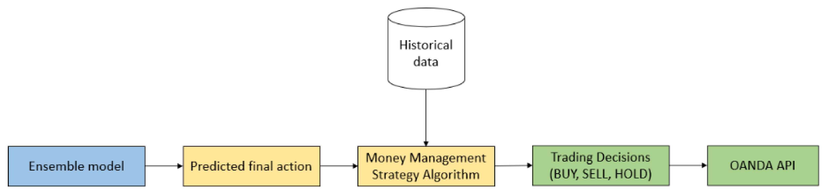
An important factor when executing trades is to limit negative risk. Therefore, the maximum drawdown of the model was restricted to a predetermined threshold. The module is also designed to be sensitive to transaction costs, thus restricting the amount of the transactions it can make. The predefined strategy inside the Money Management Strategy algorithm will use the predicted result to make trading decisions whether to buy, to sell or to hold. The overall process flow of the trader module can be visualized in
Figure 7.
3.6. Optimizer Module
There are many strategies that traders employ to trade in the Forex market. Some of the popular ones include moving average strategies such as the 50-day moving average [
44]. However, there is no guarantee that such strategies will always turn a profit despite regime or market changes. In fact, depending on the market situation, using a different moving average period other than the 50-day moving average might actually perform better. The challenge is then to decide which parameter is most optimal for the strategy to maximise profit gain. This can be viewed as an optimization problem, where the aim is to optimize a set of rules that constitute a trading strategy. An example of an optimization method to tackle this problem is the use of a GA. GAs are not good for finding patterns, but excel in exploring the solution space to search for better parameters that optimize the result. There have been past research works that attempt to use GA to optimize strategy-trading rules in the Forex market [
45,
46]. In the context of Forex trading, the GA can be broken down into the following components:
Gene: a feature parameter that defines the strategy (e.g., EMA Period);
Individual/Chromosome: represents a complete set of feature parameters to define the strategy;
Population: a collection of possible sets of feature parameters;
Parents: two sets of feature parameters that are combined to create a new feature set;
Mating pool: a collection of parents that are used to create the next generation of possible sets of feature parameters;
Fitness: a function that tells us how good the strategy performs based on the given set of feature parameters, in this case the fitness is defined by the “P&L”;
Mutation: a way to introduce variation in our population by randomly swapping two feature parameter value between two individuals;
Elitism: a way to carry the best individuals into the next generation;
CrossOver: combines parent chromosomes to create new offspring individuals.
4. System Model Design
Multiple types of supervised learning models were explored to be used in the system. Ordinary machine learning models such as support vector machine (SVM) and random forest classifier (RFC) models, which were the most common machine learning models for stock market prediction were selected as possible candidates. Prophet from Facebook, which is a time-series univariate type of model, was also explored as well. However, the results for SVM, RFC and Prophet did not show much potential in terms of profit and accuracy. As such, they are excluded from the results.
In addition, this study explored deep learning models such as CNN and LSTM, deep reinforcement learning models and conventional GA-optimized models.
4.1. Deep Learning
4.1.1. Bi-Directional LSTM
Recurrent neural network (RNN) is a type of deep learning model where its weights computed during training are adjusted based on current training example and output from previous example which causes it to have a feedback loop [
47]. This architecture conforms perfectly with the time-series nature of stock price data. A hierarchy of deep RNNs have been shown to perform well for prediction tasks as related to time-series data [
48]. The problem with RNN is the vanishing and exploding gradient problem due to the long connections between the final output layer and hidden layers of previous data in the sequence [
47]. Long short-term memory (LSTM) was then designed to overcome the vanishing gradient problem, where gates and memory units to remember the gradients are being included [
49]. Three types of gates are used in LSTM, the forget gates—remove irrelevant past information and remember only the information that is relevant for the current slot, the input gates—control the new information that acts as the input to the current state of the network; and the output gates—produce predicted value computed by the model for the current slot [
47].
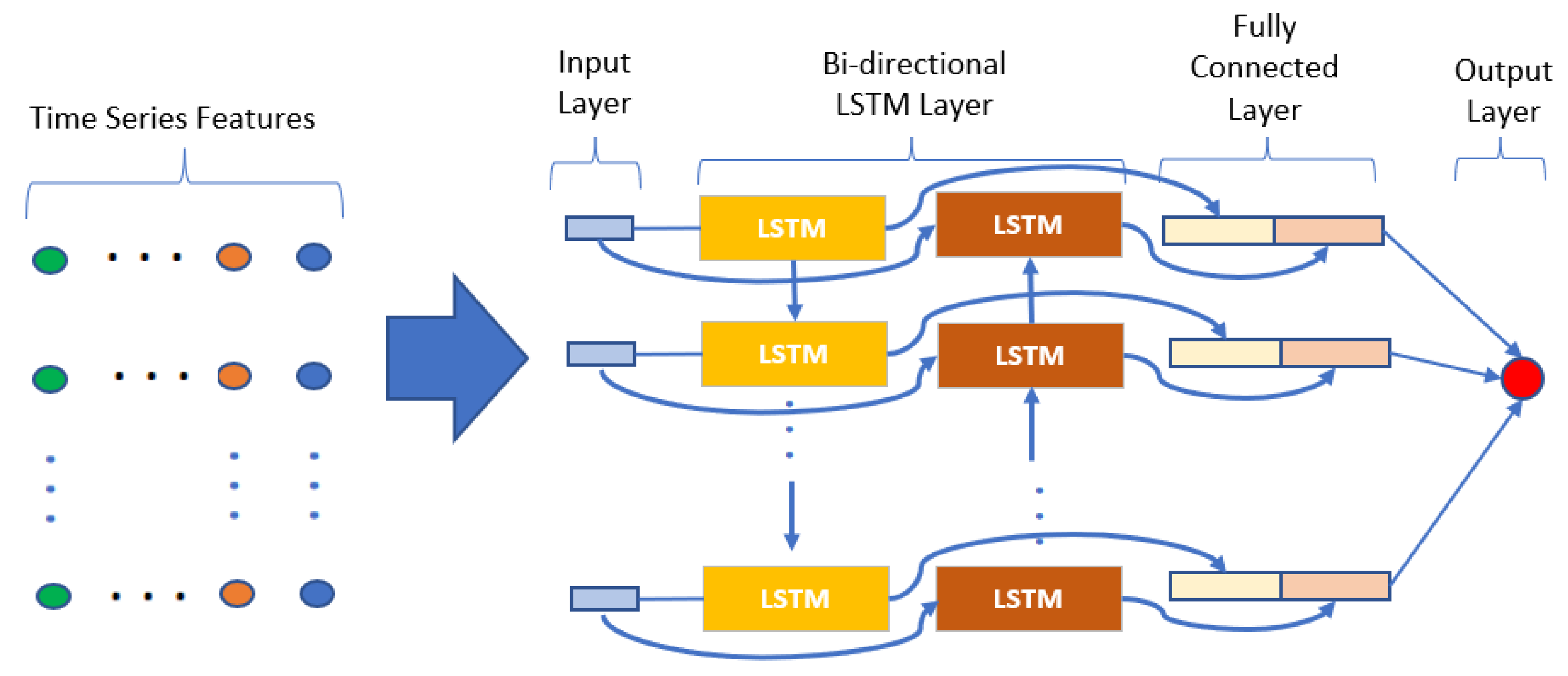
For this study, the bidirectional LSTM from [
50] is utilized. This type of bidirectional recurrent neural networks connects two hidden layers of opposite directions to the same output thus it can learn from both the forward and backward time dependencies. With this form of generative deep learning, the output layer can get information from past and future states simultaneously. In a bidirectional LSTM, each unit is split into two units having the same input and connected to the same output. One unit is used for the forward time sequence and the other for the backward sequence. The common output does an arithmetic operation such as sum, average or concatenation on both the units. Bidirectional LSTM is thus useful when learning from long spanning time-series data [
51]. This type of bidirectional LSTM was also used in other research works for stock market closing price prediction [
52]. The general bidirectional LSTM framework is illustrated in
Figure 8.
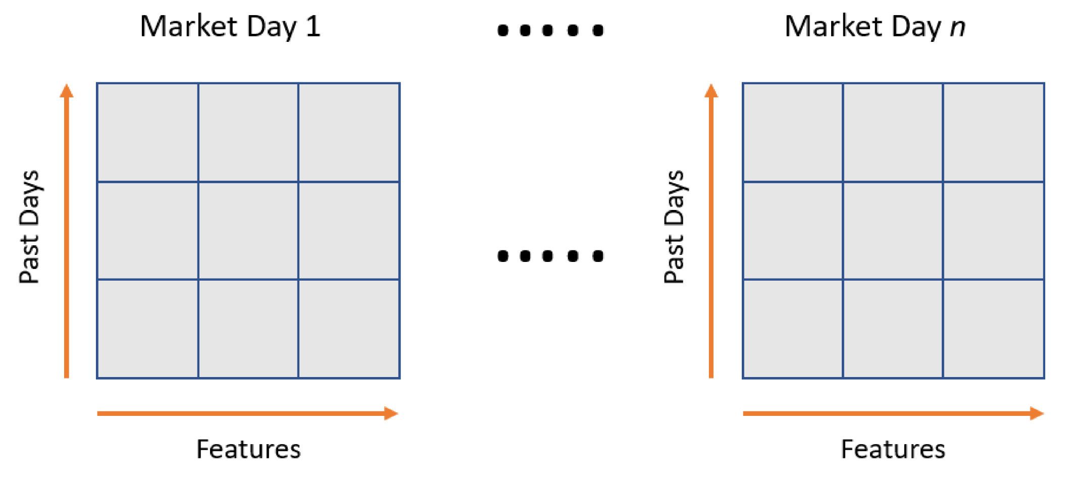
The input Forex data was shaped into a sequence of two-dimensional data (past day and features) as shown in
Figure 9. The features consist of OHLCV and technical indicators data. In this study, 30 days of past-day data was used as the look-back input. This value was selected based on a study where the authors created 30 days of sample chunks by sliding window over time series to predict the value of the 31st day [
53].
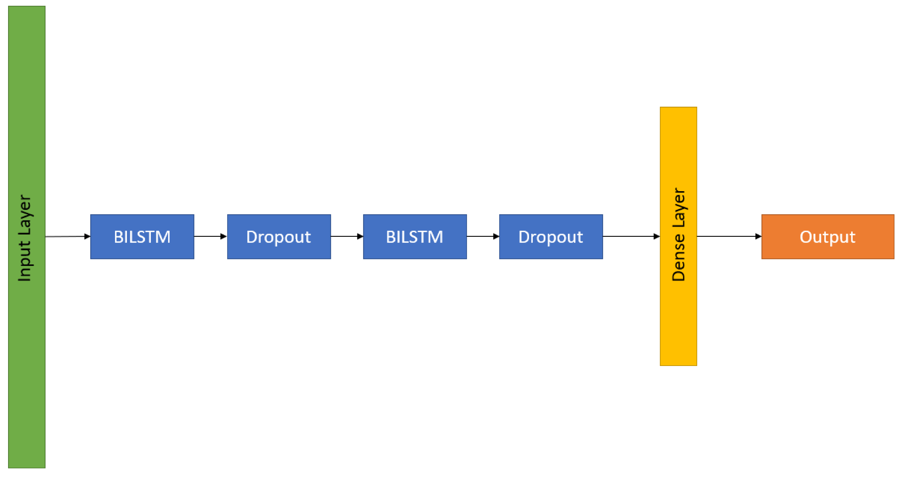
Figure 10 shows the bidirectional LSTM architecture used in this project. The return sequence parameter is set to True to obtain all the hidden states at the first LSTM layer. A drop out of 25% at the first dropout layer and 50% at the second dropout layer is added to generalize the model while minimizing overfitting.
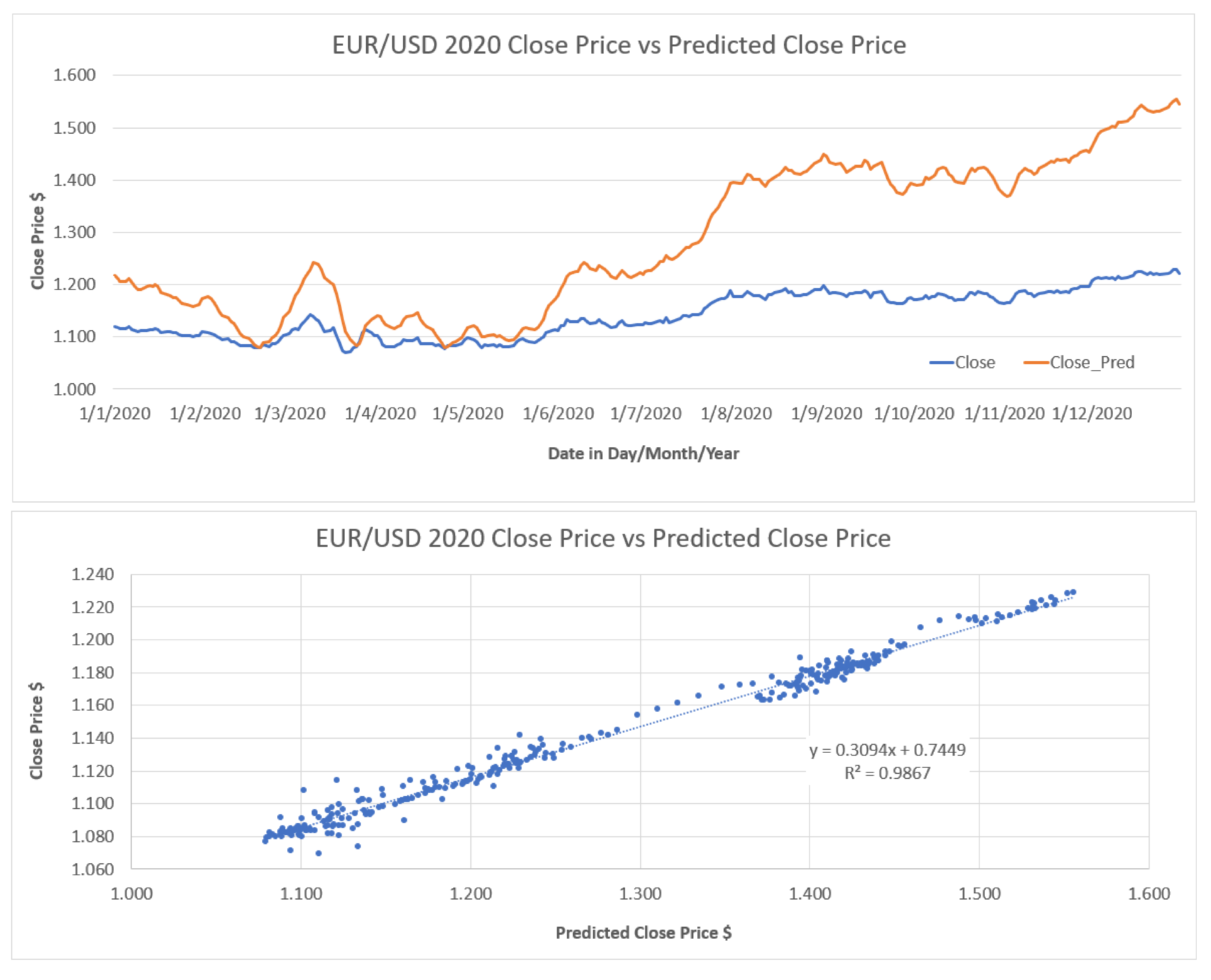
The BILSTM model was used as a regression model to predict the next day close price to obtain the Forex close price movement direction, the result is then converted to a binary Buy or Sell signal. An offset was observed between the predicted close price and the actual close price but in a linear relationship as shown in
Figure 11 below.
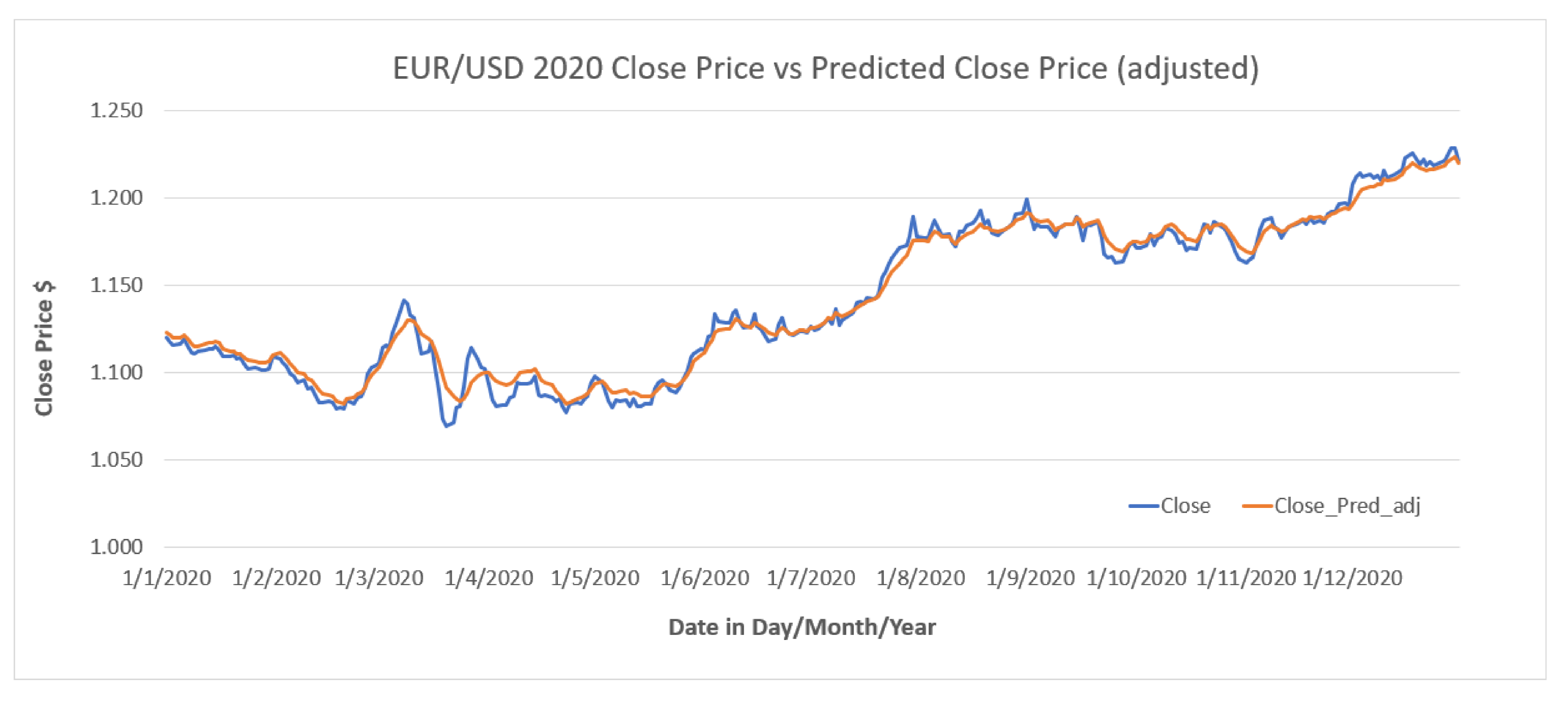
Figure 12 shows the adjusted predicted close price versus the actual close by after adjusting the predicted close price according to the linear function obtained. It is observed that there is a lag between the predicted close price (orange line) and the actual close price. This lagging phenomenon is explained in [
54], where the point-by-point prediction seems to closely match the real price curve However, this is deceptive in reality as the prediction tends to simply repeat the trajectory of historical prices with a delay. The delay occurs because the predicted price is close to the last time step of the input stock price sequence.
4.1.2. Convolutional Neural Network (CNN)
CNN is the another deep learning regression model that was explored. Compared to LSTM, CNN is a relatively new architecture used in financial time-series prediction. The major advantage of CNN over other deep learning approaches is that it can model more complex nonlinear relationships by increasing the number of layers but increasing the number of feed-forward neural networks will cause overfitting due to the number of parameters increased from the given data. CNN is able to address this issue by convoluting, downpooling and dropout operation which will allow for a deeper architecture [
55].
A CNN consists of two major processing layers—the convolutional layers and the pooling layers. The 2D convolutional layers are used for reading the inputs in the form of a sequence of two-dimensional data. The results of the reading are projected into a 2D filter map that represents the interpretation of the input. In CNN, the filters are not defined. The value of each filter is learned during the training process [
56]. Every filter is spatially small (in terms of width and height) but extends through the full depth of the input volume. During the forward pass, each filter is moved across the width and height of the input volume, and dot products are computed between the entries of the filter and the input at any position. As the filter is moved over the width and height of the input volume, a two-dimensional feature map that gives the responses of that filter is produced at every spatial position [
57]. The pooling layers operate on the extracted feature maps and derive the most essential features by averaging (average pool) or max computing (max pooling) operations.
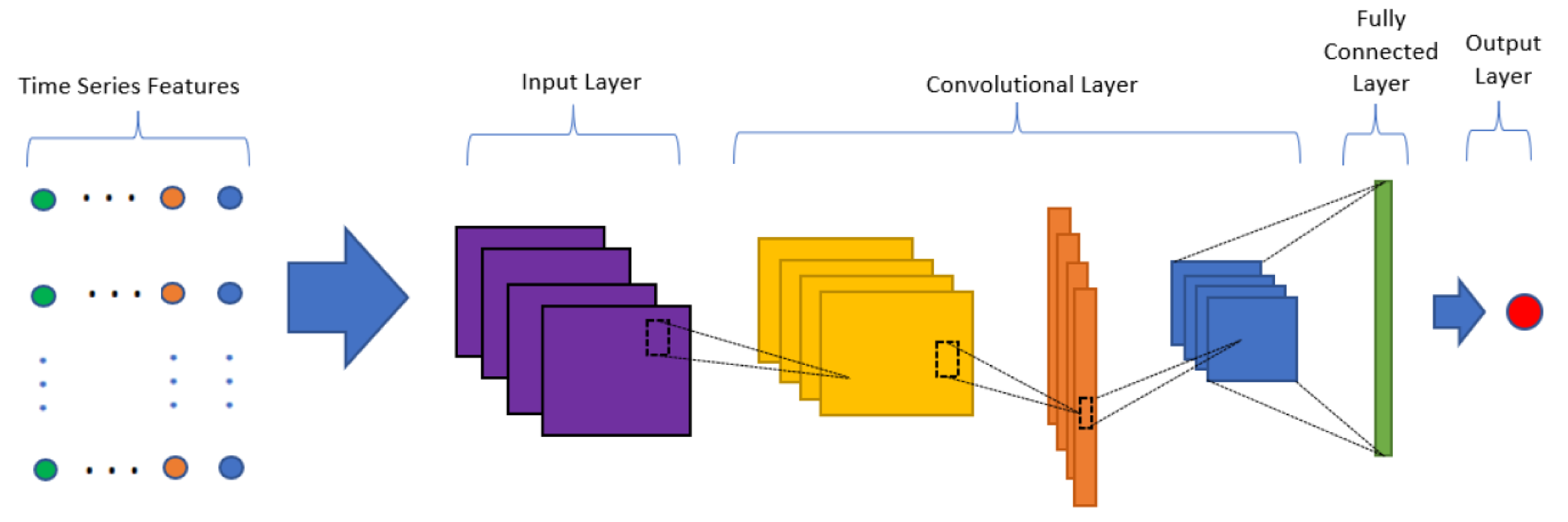
Figure 13 illustrates the high level architecture of a CNN model for Forex time series applications.
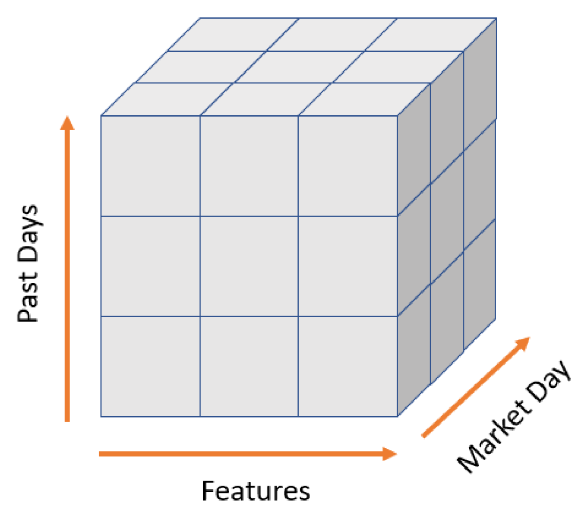
To feed the time-series data into the CNN model, we reshaped the multivariate input data, and the time-series features data was turned into images in sequence as shown in
Figure 14. An example of Forex features’ data presented in image form, with 30 days of past day and features which consists of OHLCV and the technical indicators is presented in
Figure 15.
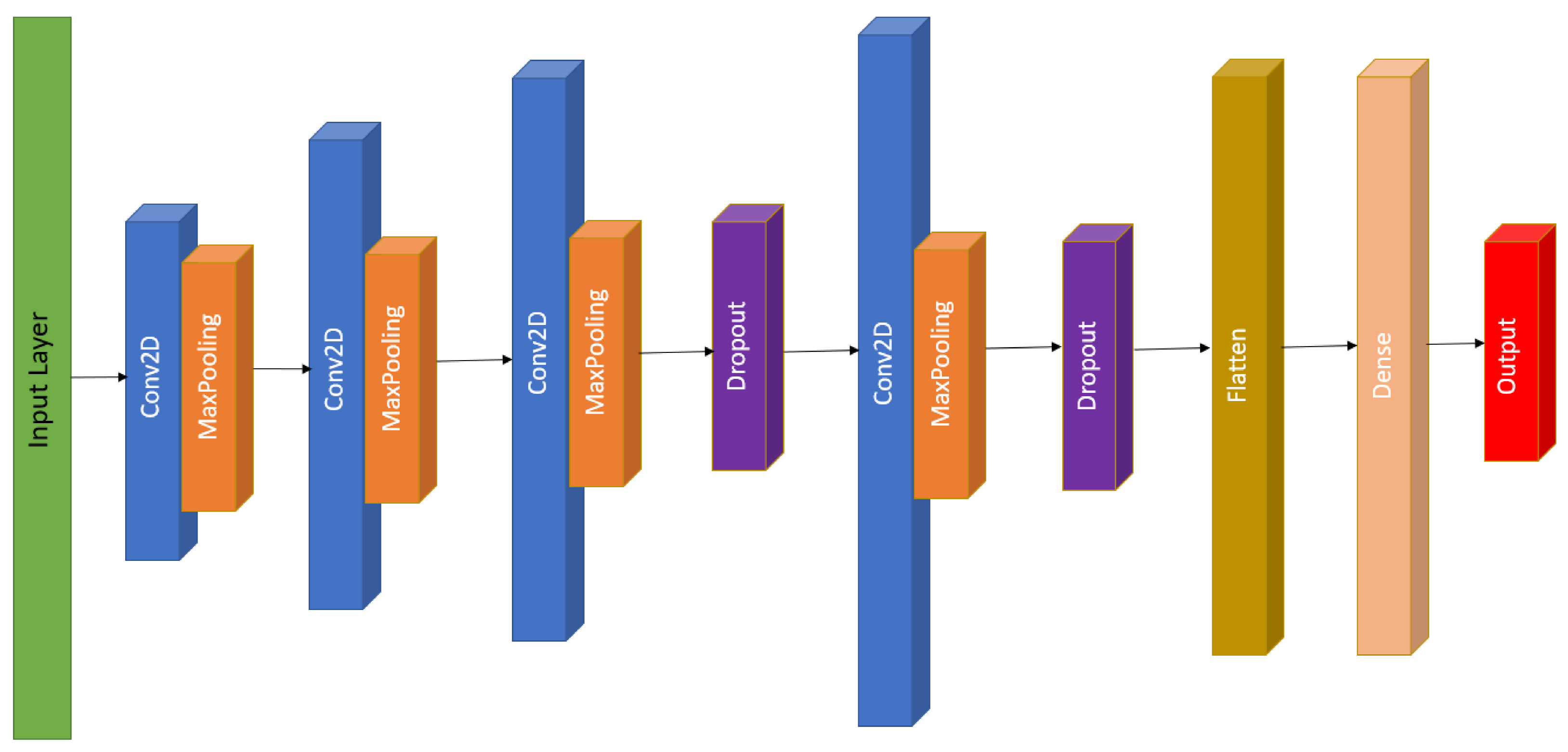
The CNN based regression model consists of four convolutional layers with kernel sizes of 32, 64, 128 and 256 and with a filter size of 1 as shown in
Figure 16. Dropout rates of 25% and 50% were introduced at the last two layers to generalize the model. The rectified linear unit (ReLU) function has been used in the convolution and fully connected layer, the performance of the layers is optimized by using ADAM optimizer, both the activation and optimizer were chosen with reference to [
47,
51] CNN models used in stock price prediction. For extracting deep features from the input sequence, the convolution and the pooling layers may be repeated multiple times. The output from the last pooling layer is sent to one or more dense layer(s) for extensive learning from the input data.
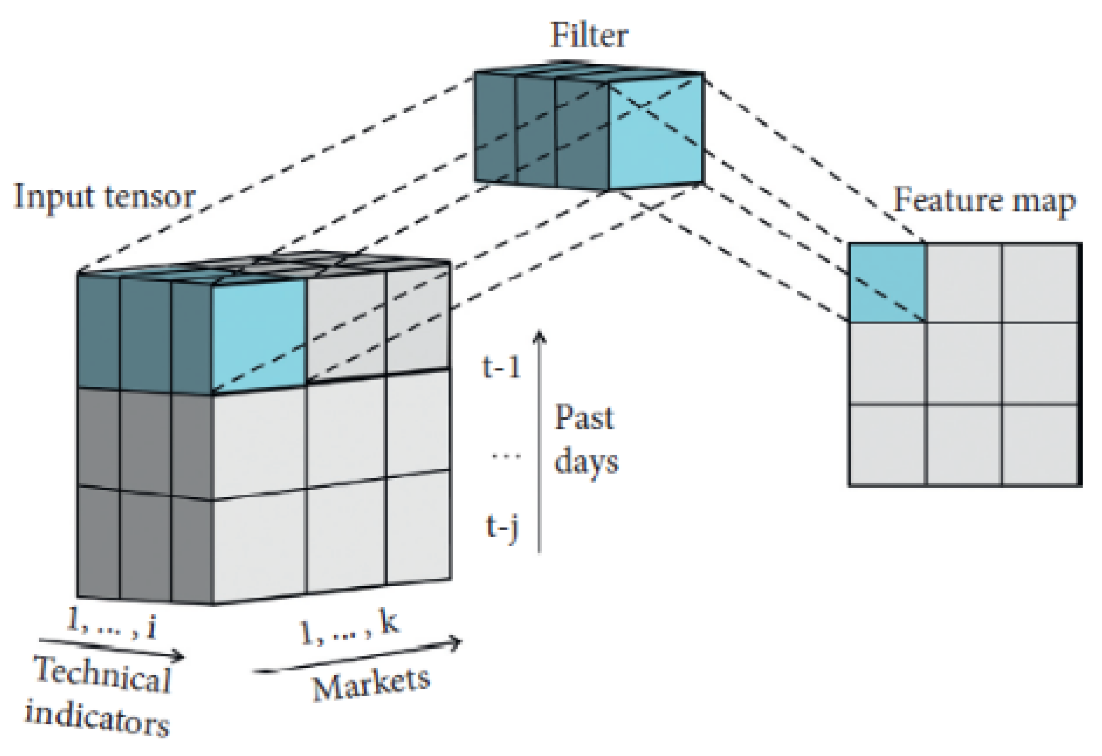
The size of the pooling layer is set as 1 (which is equivalent to no pooling) because [
58] claimed in the financial study that if a pooling layer is adopted, the information would probably be lost. Specifically, the convolutional layer is designed for performing convolution operations on the input data. The convolution operation can be considered as a filter used for the input data. The size of a filter suggests its coverage.
Figure 17 shows how the 1 × 1 filter works in the three-dimensional input tensor [
59].
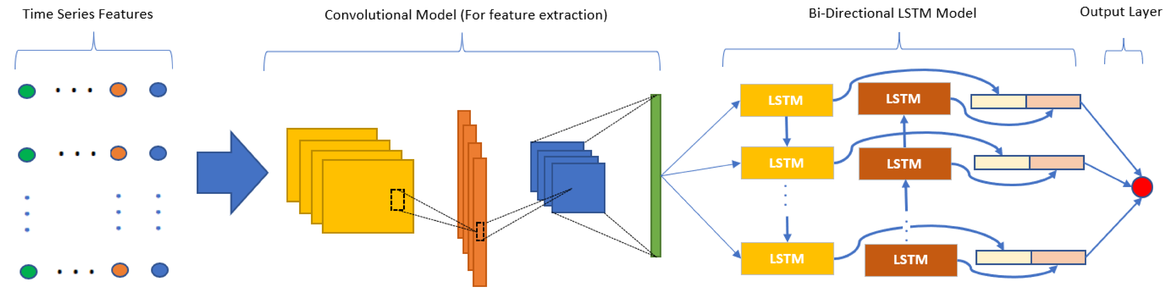
4.1.3. CNN-BILSTM
A hybrid model, which comprised CNN for feature extraction and BILSTM for prediction, was explored. This hybrid model has also been used by another research works in stock market prediction [
51,
59]. A pure LSTM-based regression model reads the input sequential data directly, and computes the internal state and state transitions to produce its predicted sequence but a CNN-LSTM model extracts the features from the input sequence using a CNN encoder submodel, and then interprets the output from the CNN models. The output from the CNN model will be passed to LSTM as input. In contrast to these, a convolutional LSTM model uses convolution operation to directly read a sequential input into a decoder LSTM submodel [
47].
Figure 18 illustrates the CNN-LSTM architecture. The data was reshaped to 3D using the same methodology described for the CNN model.
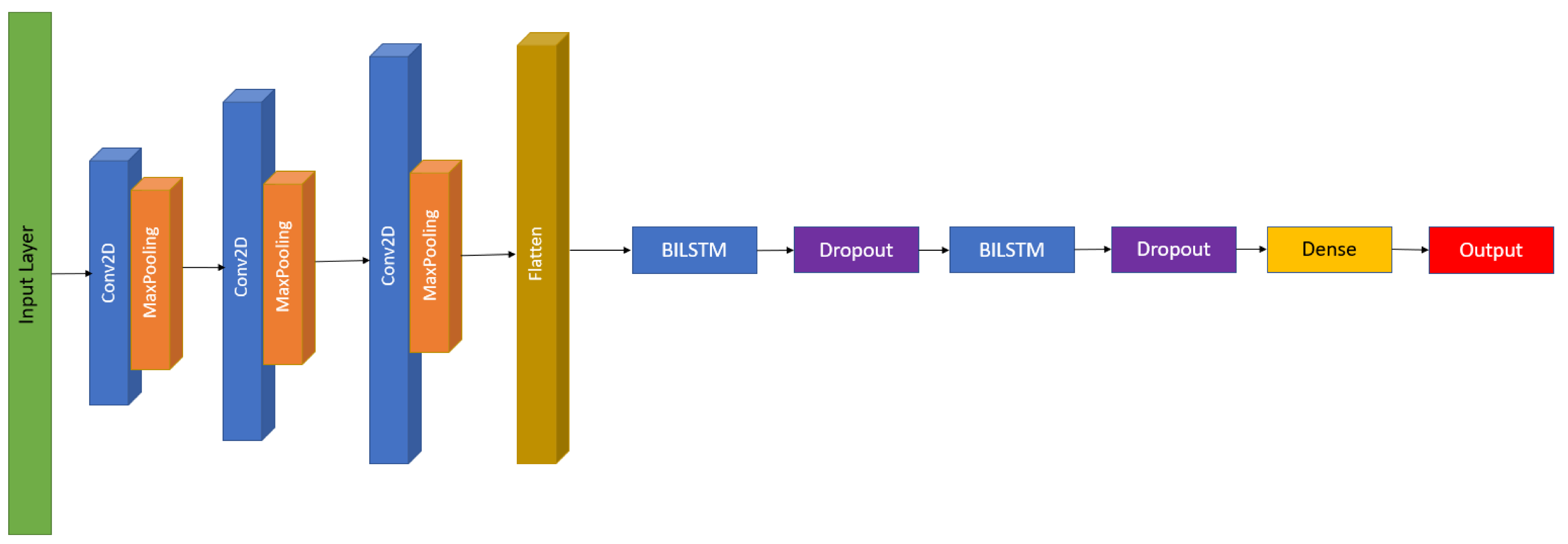
For the CNN-BILSTM hybrid model, three convolutional layers are used, and the number of filters for each convolutional layer is 128, 256 and 512, respectively. The number of filters is based on the hybrid CNN-LSTM model used in [
51]. The kernel size is one, which is the same as CNN model and explained in
Section 4.1.2. The output of the CNN submodel will be flattened before connecting to the BILSTM submodel. The BILSM submodel here is the same as the one described previously, with the same dropout rate of 25% and 50% before the output layer. The architectural framework of the CNN-BILSTM model is shown in
Figure 19.
4.2. Reinforcement Learning
Reinforcement learning (RL) is a type of machine learning technique that enables an agent to learn in an interactive environment by trial and error using feedback mechanisms from its own actions and experiences, reinforced by rewards given by the environment as a result of the agent’s action [
60]. Deep reinforcement learning (DRL) is an extension of RL, which consists of a combination of both reinforcement learning and deep learning. Since the objective of financial trading is to maximise profit and minimise losses, this makes RL very applicable in the context of financial trading.
For this study, a value-based algorithm (DQN: Deep Q-Networks), an actor–critic reinforcement learning algorithm (A2C: advantage actor critic) and a policy-based algorithm (PPO: proximal policy optimization) were selected to be explored. The reason for these selected approaches is to be able to observe and evaluate representative model from each type of RL.
Value-based RL: objective is to learn the state-value or state-action-value function to generate the most optimal policy.
Policy-based RL: aims to learn the policy directly (policy determines what action to take at a particular state, it is a mapping from a state to an action) using parameterized functions.
Actor–critic RL: aims to learn both value and policy by deploying one neural network as the actor which takes action and another neural network acting as the critic to adjust the action that the actor takes.
The selected RL models are trained on EURUSD market data from 2017–2019, and subsequently evaluated on 2020 data. All the RL models use 20 historical data points and 4 technical indicators (EMA20, RSI, MACD, and SIGNAL) taken from finta python library.
4.2.1. Deep Q-Networks (DQN)
DQN is based on Q-Learning to obtain the optimal policy (action-value function). In a finite state, it is possible to obtain the q* which is the optimal policy for the agent to reap the most possible reward. However, in real-world problems, the state of action-value is often enormous and practically unlimited. This has made it impossible to store the action-value pair for any possible state. Thus, DQN model utilises deep neural network as a universal function approximator to replace the Q table. DQN has two separate networks with the same architecture. One is to estimate the target and another one is to predict the Q values. The result from the target model is utilised as the ground truth for the prediction network. The prediction network’s weights are updated in every iteration whilst the target network’s weights will be updated based on prediction network’s weights after a certain N number of iterations, which is part of the model’s hyperparameter.
4.2.2. Advantage Actor Critic (A2C)
The A2C model is a reinforcement learning model which combines actor-only (policy-based) and critic-only (value-based) approaches. An actor-only approach means having a neural network learn the policy where policy represents a probability distribution of taking a particular action given a state. A critic-only approach means using a Q-value function to learn the optimal action-selection policy that maximizes the expected future reward given the current state. Combining the above, an actor–critic approach behaves such that the critic estimates the value function (which can be Q-value or state-value) and then the actor updates the policy distribution in the direction suggested by the critic. The actor–critic algorithm is represented as two networks, the actor network and the critic network which work together to solve a particular problem. The A2C model utilizes advantage function to reduce the variance of policy gradient. Advantage function is calculated by measuring the temporal difference error (TD Error). TD error is calculated by the predicted value of all future rewards from the current state S (TD Target) minus the value of the current state S.
4.2.3. Proximal Policy Optimization (PPO)
PPO Model uses policy gradient update in a controlled manner such that after an update, as such the new policy should be not too far from the old policy. PPO controls fluctuations by discouraging large policy changes using a clipping mechanism (clipped interval) to improve the stability of policy networks training.
4.3. Genetic Algorithm (GA)
Trade optimization in the form of GA can be deployed with any conventional rule-based trading algorithms. This will be a major advantage for trading houses to have the ability to optimize their existing proven rule-based strategies. For this study, the conventional pullback strategy was selected to be optimized.
Pullback Strategy
One of the most common ways to trade financial markets is the use of a pullback strategy. A “pullback” is defined as a pause or moderate drop in a stock or commodities pricing chart from recent peaks that occur within a continuing uptrend or downtrend [
61]. The concept behind a pullback strategy is to identify when a pullback is going to occur, which indicates a signal to “sell” since the price is expected to decrease, as well as when the reversal of the pullback, which indicates a signal to “buy” since the price is expected to increase.
One possible pullback strategy involves the use of exponential moving average (EMA) and relative strength index (RSI) technical indicators. The EMA is used for trend direction and a fast-period RSI is used to identify the onset of a pull back. The rules of this pullback strategy at any certain point of time is as follows:
If “Close price” > “EMA value” and “RSI value” < “RSI_buy_threshold_value”, THEN “BUY”
ELIF “RSI value” < “RSI_sell_threshold_value”, THEN “SELL”
ELSE “BUY”
The pullback strategy parameters are modeled as GA chromosomes for the GA optimizer. Optimization is done with a population size of 20 over 5 generations. The period chosen to optimize parameters is on 2019 data. The fitness function used to define the reward value is the P&L produced by trading during the period of the training dataset. The optimized parameters after running the GA optimizer on the Pullback strategy is outlined in
Table 1:
5. Results
5.1. Experimental Setup
The dataset used for evaluation consists of OHLCV data for EURUSD Forex pair ranging from January 2020 to December 2020 [
62]. The raw data was harvested from OANDA and pre-processed accordingly as described previously in
Section 3.3.2 and
Section 3.3.3. The preprocessed data is then passed into the strategy to obtain a predicted action, which is then passed onto the trader module as described in
Section 3.5 to execute the action. For each strategy, accuracy and profitability metrics are extracted to evaluate the overall performance.
The key trading parameters used for the backtesting evaluation are listed in
Table 2.
5.2. Time-Series Univariate Results Analysis
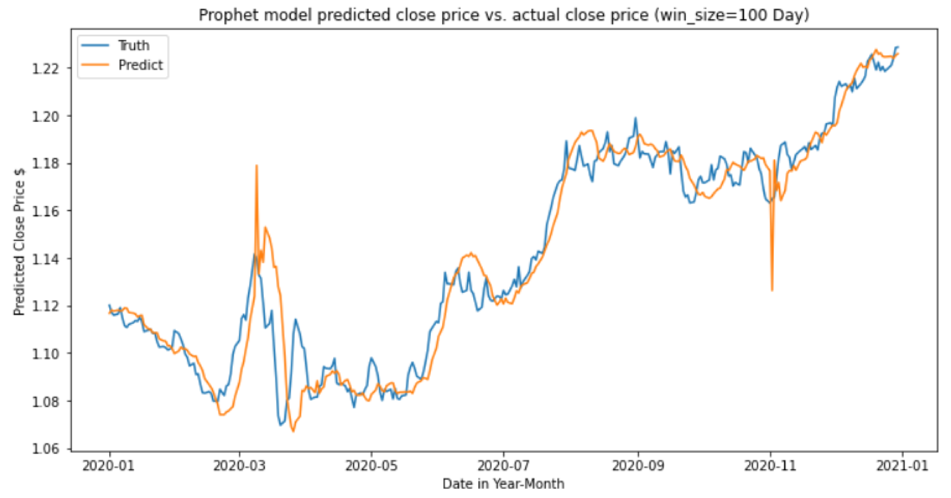
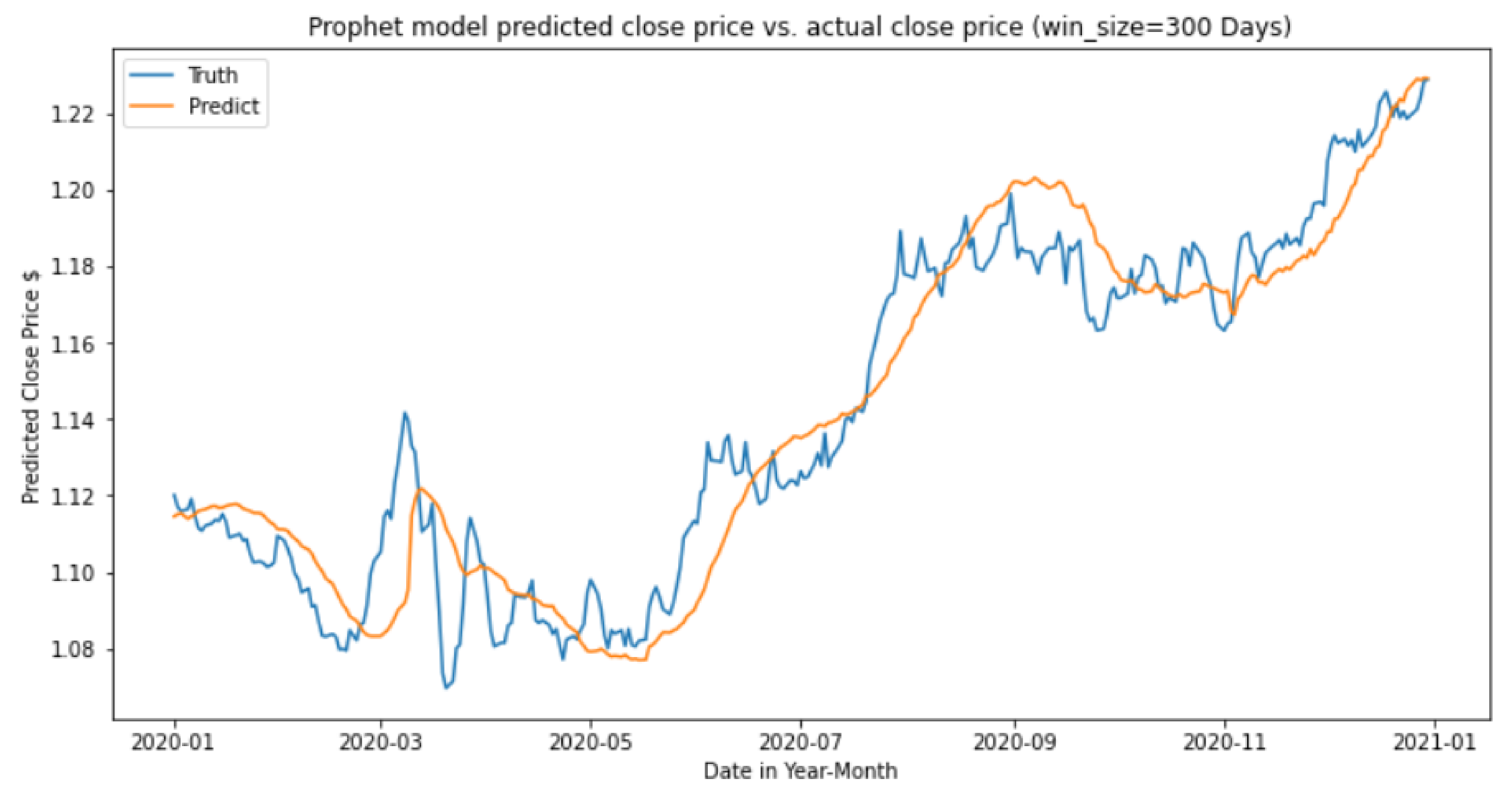
The forecasting chart in
Figure 20 and
Figure 21 shows the prediction result using the Prophet model with a window period of 100 days and 300 days. Using a period of 100 days for the window period, the predicted trend seems to be closer to the actual ground truth trend. However, there is noise present within the predicted trend. In contrast, using a window period of 300 days, the predicted trend becomes smoother, reducing the amount of noise. However, this produces a notable lag between the predicted and actual trends as indicated by the offset.
Based on test data from the year 2020, the Prophet model with a 300-day window period performed better, with an F1 score of 0.55 and 3.86% of Nett profit and loss. In contrast, the Prophet model with a 100-day window period obtained an F1 score of 0.52 and only 1% of Nett profit and loss.
5.3. Strategies Performance Comparison
Since the system utilizes an ensemble method to predict the market signal for the next day, the seven strongest-performing models are selected to be included inside the ensemble with a simple majority voting mechanism. The number of models selected is purposely made as an odd number so that at any point, there will always be a clear winner (either Buy or Sell action). All the models achieve positive result for the test period of 2020 with opening capital of 5,000,000. The performance results for each individual strategy as well as the ensemble strategy is outlined below in
Table 3:
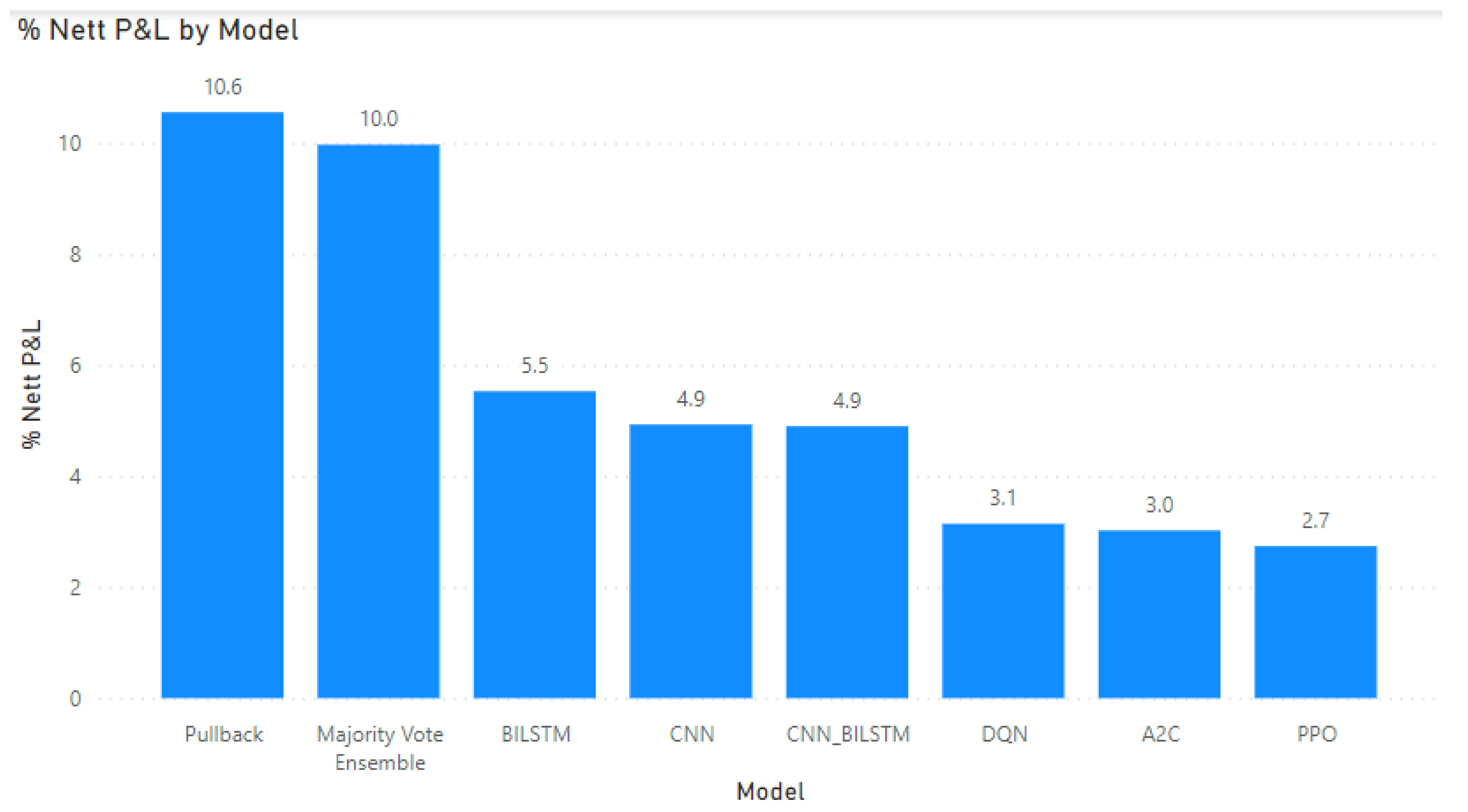
With regards to the profitability performance of the models, based on the results visualization in
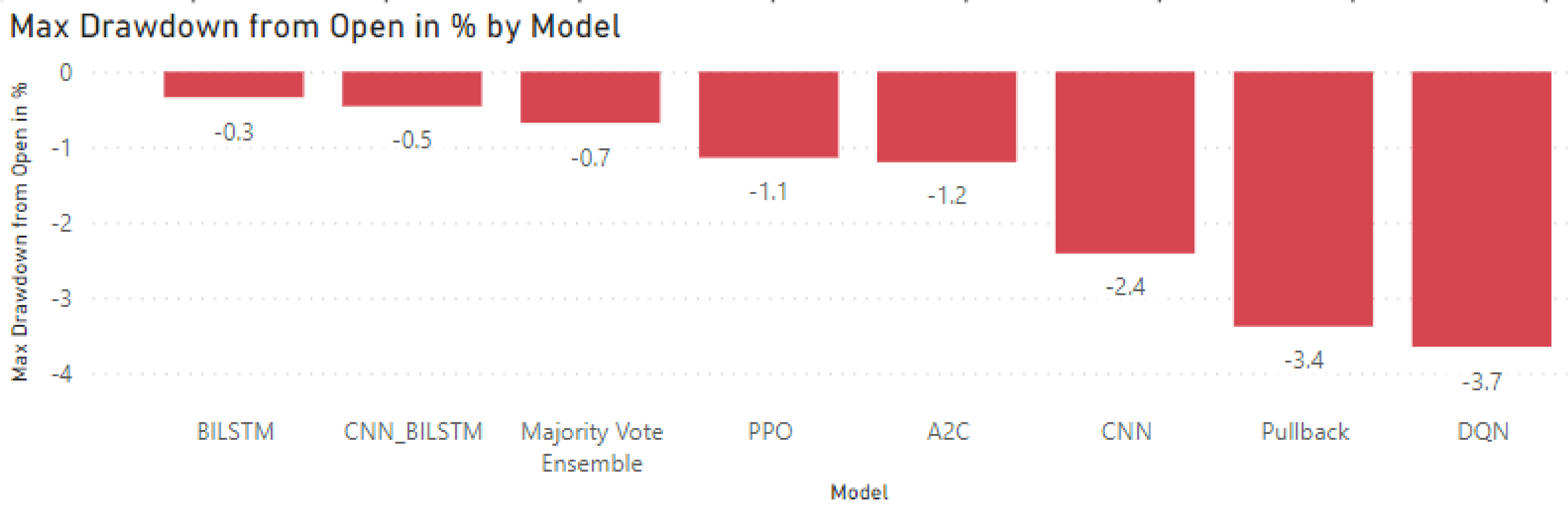
Figure 22, it is noted that all models are able to achieve profitable results for 2020 test data samples. The best profitability is achieved by pullback strategy using genetic algorithm technique, which obtained a 10.6% Nett P&L. Excellent result were also observed for drawdown (maximum floating loss) as seen in
Figure 23, where all models achieved less than 5% drawdown from initial capital. In addition, by using an Ensemble approach with simple majority vote, it resulted in profitability close to the best model (Pullback strategy with GA) and with much better drawdown level (less floating loss percentage), where drawdown was only −0.7% for the ensemble as compared to −3.4% drawdown for pullback strategy.
With regards to the accuracy performance of the models, based on the results visualization in
Figure 24, it is noted that all models achieved an overall accuracy level of more than 50%, which means they have the edge to achieve profitability compared to a random guess. In addition, all models’ F1 Scores for Buy are also higher than 0.5, signifying the edge of the models’ predictive power over random guessing during 2020 test data. In a general sense, with a higher accuracy and F1 score, it should lead to better profitability. The results for overall accuracy and the F1 score for buy action show the above correlation. However the F1 score for sell action does not show the correlation because the 2020 EUR/USD trading data was in an upwards trend, thus it was more profitable for the models to perform the buy action rather than sell action.
6. Discussions and Conclusions
Predicting the market movement of Forex pair is a complex but necessary task in order to generate profits. This study presents AlgoML, a complete end-to-end intelligent system solution for automated Forex trading, which aims to improve upon pre-existing rule-based systems to increase profitability through the use of ML-based decision making and a robust money management strategy.
An ensemble approach is employed for the decision making of the system, where each strategy takes in preprocessing technical data to output an independent buy or sell signal. The strategies/models deployed include a mix of reinforcement learning, supervised learning and GA-optimized conventional techniques. The signals from each strategy is then collated into the ensemble model, which utilizes a majority voting logic to determine the final predicted action to be taken. The final action is then passed into the money management strategy to decide on the final trade action parameters, which the system passes through a trade broker API to perform the actual trade. An intuitive front-end integrated UI is developed to allow traders to easily use AlgoML to make predictions and execute trades in a quick and systematic process. Based on backtest results, AlgoML has demonstrated strong potential in achieving profitability.
In addition to showing high promise in being a profitable solution, the work presented in this study outlines a flexible system architecture; where different strategies for predicting market signal or money management can be easily plugged in and out to observe their impact during backtesting evaluation. This means that other organizations or research studies that might have already developed their own prediction or money management strategies can adapt it to AlgoML’s existing architecture. As such, it would serve as a good foundation to build different automated Forex trading system solutions.
One area for future work to improve upon AlgoML is the development of a more dynamic money management strategy. This could be in the form of more aggressive or more conservative stances that the strategy would take. For example, if the market is in an uptrend, the strategy could be willing to risk more due to the positive conditions. In contrast, if the market is in a recession, the strategy would adopt a more conservative stance to minimize losses amid the negative conditions.
Another possible area of future work is the exploration of strategies to analyze market sentiment based on news reports. External events such as regime change or natural disasters can have an impact on the currency pair exchange rate [
63]. Thus, this opens up the possibility to develop NLP-based strategies to analyze the sentiment and expected impact on the Forex market through news reports on such events.
In summary, this study presents a complete end-to-end system for automated Forex trading, along with a highly flexible architecture that can be utilized as a solid foundation to develop and backtest different kinds of Forex trading system solutions. The results show that high profitability of the system and that it can be deployed for actual real-life trading purposes.
Author Contributions
Conceptualization, L.K.Y.L., H.K.K., N.J.P., H.C.; methodology, L.K.Y.L., H.K.K., N.J.P., H.C.; software, L.K.Y.L., H.K.K., N.J.P., H.C.; validation, L.K.Y.L., H.K.K., N.J.P., H.C.; formal analysis, L.K.Y.L., H.K.K., N.J.P., H.C.; investigation, L.K.Y.L., H.K.K., N.J.P., H.C.; resources, L.K.Y.L., H.K.K., N.J.P., H.C.; data curation, L.K.Y.L., H.K.K., N.J.P., H.C.; writing—original draft preparation, L.K.Y.L., H.K.K., N.J.P., H.C.; writing—review and editing, L.K.Y.L., H.K.K., N.J.P., H.C., M.C.H.C., N.J.H.H.; visualization, L.K.Y.L., H.K.K., N.J.P., H.C.; supervision, M.C.H.C., N.J.H.H.; project administration, M.C.H.C., N.J.H.H. All authors have read and agreed to the published version of the manuscript.
Funding
This research received no external funding.
Institutional Review Board Statement
Not applicable.
Informed Consent Statement
Not applicable.
Data Availability Statement
Not applicable.
Acknowledgments
The authors would like to acknowledge PH7 for sponsoring this project and providing subject matter expertise and guidance.
Conflicts of Interest
The authors declare no conflict of interest.
Abbreviations
The following abbreviations are used in this manuscript:
| SOTA | State of the Art |
| SME | Subject Matter Expert |
| Forex | Foreign Exchange Market |
| OHLCV | Open, High, Low, Close, Volume |
| P&L | Profit and Loss |
| ML | Machine Learning |
| DL | Deep Learning |
| RL | Reinforcement Learning |
| DRL | Deep Reinforcement Learning |
| RFC | Random Forest Classifer |
| SVM | Support Vector Machine |
| IID | Independent and identically distributed |
| GA | Genetic Algorithm |
| CNN | Convolution Neural Network |
| LSTM | Long Short-term Memory |
| BiLSTM | Bi-Directional Long Short-term Memory |
| ETL | Extract, Transform and Load |
| ADF | Augmented Dickey-Fuller |
| MA | Moving Average |
| EMA | Exponential Moving Average |
| RSI | Relative Strength Index |
References
- Folger, J. 10 Ways to Avoid Losing Money in Forex; Investopedia: New York, NY, USA, 2021. [Google Scholar]
- Kuepper, J. Risk Management Techniques for Active Traders; Investopedia: New York, NY, USA, 2021. [Google Scholar]
- Hayes, A. Forex Trading Robot; Investopedia: New York, NY, USA, 2021. [Google Scholar]
- What Is Automated Trading? Available online: https://www.ig.com/sg/trading-platforms/algorithmic-trading/what-is-automated-trading (accessed on 29 January 2022).
- Chou, Y.H.; Kuo, S.Y.; Chen, C.Y.; Chao, H.C. A Rule-Based Dynamic Decision-Making Stock Trading System Based on Quantum-Inspired Tabu Search Algorithm. Access IEEE 2014, 2, 883–896. [Google Scholar] [CrossRef]
- Wilson, J. How Much Artificial Intelligence Has Changed the Forex Trade. Aithority 2020. Available online: https://aithority.com/guest-authors/how-much-artificial-intelligence-has-changed-the-forex-trade/ (accessed on 29 January 2022).
- Rabin, K. How Is AI Revolutionizing FX Market in a Way We Didn’t Even Realize; Finextra: London, UK, 2021. [Google Scholar]
- Fetalvero, N. Here’s how tech has revolutionized forex trading. Tech Asia 2020. Available online: https://www.techinasia.com/heres-tech-revolutionized-forex-trading (accessed on 29 January 2022).
- Escudero, P.; Alcocer, W.; Paredes, J. Recurrent Neural Networks and ARIMA Models for Euro/Dollar Exchange Rate Forecasting. Appl. Sci. 2021, 11, 5658. [Google Scholar] [CrossRef]
- Deka, A.; Resatoglu, N. Forecasting Foreign Exchange Rate And Consumer Price Index With Arima Model: The Case Of Turkey. Int. J. Sci. Res. Manag. 2019, 7, 1254–1275. [Google Scholar] [CrossRef]
- Cao, L.; Tay, F. Financial Forecasting Using Support Vector Machines. Neural Comput. Appl. 2001, 10, 184–192. [Google Scholar] [CrossRef]
- Kamruzzaman, J.; Sarker, R. ANN-Based Forecasting of Foreign Currency Exchange Rates. Neural Inf.-Process.-Lett. Rev. 2004, 3, 49–58. [Google Scholar]
- Thu, T.N.T.; Xuan, V.D. Using support vector machine in FoRex predicting. In Proceedings of the 2018 IEEE International Conference on Innovative Research and Development (ICIRD), Bangkok, Thailand, 11–12 May 2018; pp. 1–5. [Google Scholar] [CrossRef]
- Juszczuk, P.; Kozak, J.; Trynda, K. Decision Trees on the Foreign Exchange Market; Springer: Cham, Switzerland, 2016; pp. 127–138. [Google Scholar] [CrossRef]
- Nti, I.K.; Adekoya, A.; Weyori, B. A comprehensive evaluation of ensemble learning for stock-market prediction. J. Big Data 2020, 7, 1–40. [Google Scholar] [CrossRef]
- Qi, L.; Khushi, M.; Poon, J. Event-Driven LSTM for Forex Price Prediction. In Proceedings of the 2020 IEEE Asia-Pacific Conference on Computer Science and Data Engineering (CSDE), Gold Coast, Australia, 16–18 December 2020; pp. 1–6. [Google Scholar]
- Zeng, Z.; Khushi, M. Wavelet Denoising and Attention-based RNN-ARIMA Model to Predict Forex Price. In Proceedings of the 2020 International Joint Conference on Neural Networks (IJCNN), Glasgow, UK, 19–24 July 2020. [Google Scholar]
- Islam, M.; Hossain, E. Foreign exchange currency rate prediction using a GRU-LSTM hybrid network. Soft Comput. Lett. 2021, 3, 100009. [Google Scholar] [CrossRef]
- Carapuço, J.; Neves, R.; Horta, N. Reinforcement learning applied to Forex trading. Appl. Soft Comput. 2018, 73, 783–794. [Google Scholar] [CrossRef]
- Théate, T.; Ernst, D. An application of deep reinforcement learning to algorithmic trading. Expert Syst. Appl. 2021, 173, 114632. [Google Scholar] [CrossRef]
- Yuan, Y.; Wen, W.; Yang, J. Using Data Augmentation Based Reinforcement Learning for Daily Stock Trading. Electronics 2020, 9, 1384. [Google Scholar] [CrossRef]
- Rundo, F. Deep LSTM with Reinforcement Learning Layer for Financial Trend Prediction in FX High Frequency Trading Systems. Appl. Sci. 2019, 9, 4460. [Google Scholar] [CrossRef]
- Downey, L. Transaction Costs; Investopedia: New York, NY, USA, 2021. [Google Scholar]
- Maurer, T.A.; Pezzo, L.; Taylor, M.P. Importance of Transaction Costs for Asset Allocations in FX Markets. In Econometric Modeling: Capital Markets—Portfolio Theory eJournal; Elsevier: Amsterdam, The Netherlands, 2019. [Google Scholar]
- Brownlee, J. A Gentle Introduction to Imbalanced Classification. Machine Learning Mastery. 2019. Available online: https://machinelearningmastery.com/what-is-imbalanced-classification/ (accessed on 29 January 2022).
- Tzveta, I. An Introduction to Non-Stationary Processes; Investopedia: New York, NY, USA, 2022. [Google Scholar]
- Brownlee, J. How to Remove Trends and Seasonality with a Difference Transform in Python. 2017. Available online: https://machinelearningmastery.com/remove-trends-seasonality-difference-transform-python/ (accessed on 29 January 2022).
- Palachy, S. Detecting Stationarity in Time Series Data. 2019. Available online: https://towardsdatascience.com/detecting-stationarity-in-time-series-data-d29e0a21e638 (accessed on 29 January 2022).
- Mushtaq, R. Augmented Dickey Fuller Test. SSRN Electron. J. 2011. [Google Scholar] [CrossRef]
- Ng, R. RAPID Fractional Differencing to Minimize Memory Loss While Making a Time Series Stationary. 2019. Available online: https://medium.com/rapids-ai/rapid-fractional-differencing-to-minimize-memory-loss-while-making-a-time-series-stationary-2052f6c060a4 (accessed on 29 January 2022).
- Baasher, A.; Fakhr, M. Forex trend classification using machine learning techniques. In Proceedings of the 11th WSEAS International Conference on Applied Computer Science, Penang, Malaysia, 3–5 October 2011; World Scientific and Engineering Academy and Society (WSEAS): Stevens Point, WI, USA, 2011; pp. 41–47. [Google Scholar]
- Sezer, O.; Ozbayoglu, M. Algorithmic Financial Trading with Deep Convolutional Neural Networks: Time Series to Image Conversion Approach. Appl. Soft Comput. 2018, 70, 525–538. [Google Scholar] [CrossRef]
- Yu, L.; Wang, S.; Lai, K. Foreign-Exchange-Rate Forecasting with Artificial Neural Networks; International Series in Operations Research & Management Science; Springer: Berlin/Heidelberg, Germany, 2007. [Google Scholar]
- Peerchemist. Finta. 2021. Available online: https://github.com/peerchemist/finta (accessed on 29 January 2022).
- Twopirllc. Pandas-ta. 2021. Available online: https://github.com/twopirllc/pandas-ta (accessed on 29 January 2022).
- Chollet, F. Deep Learning with Python; Manning Publications: Greenwich, CT, USA, 2017. [Google Scholar]
- Krizhevsky, A.; Sutskever, I.; Hinton, G. ImageNet Classification with Deep Convolutional Neural Networks. In Proceedings of the 25th International Conference on Neural Information Processing Systems–Volume 1, Nevada, CA, USA, 3–6 December 2012. [Google Scholar]
- Gan, K.; On, C.; Anthony, P.; Chang, S. Homogeneous Ensemble FeedForward Neural Network in CIMB Stock Price Forecasting. In Proceedings of the 2018 IEEE International Conference on Artificial Intelligence in Engineering and Technology (IICAIET), Kota Kinabalu, Malaysia, 8 November 2018; pp. 1–6. [Google Scholar] [CrossRef]
- Yang, J.; Rao, R.; Pei, H.; Ding, P. Ensemble Model for Stock Price Movement Trend Prediction on Different Investing Periods. In Proceedings of the 2016 12th International Conference on Computational Intelligence and Security (CIS), Wuxi, China, 16–19 December 2016; pp. 358–361. [Google Scholar] [CrossRef]
- Anzél, K. Top risk management strategies in forex trading. IG 2020. Available online: https://www.ig.com/en/trading-strategies/top-risk-management-strategies-in-forex-trading-200630 (accessed on 29 January 2022).
- Belk, P. The organisation of foreign exchange risk management: A three-country study. Manag. Financ. 2002, 28, 43–52. [Google Scholar] [CrossRef]
- Dash, M.; Kodagi, M.; Babu, N. An Empirical Study of Forex Risk Management Strategies. Indian J. Financ. 2008, 2. Available online: https://ssrn.com/abstract=1326462 (accessed on 29 January 2022).
- Al-Momani, R.; Gharaibeh, M. Foreign exchange risk management practices by Jordanian nonfinancial firms. J. Deriv. Hedge Funds 2008, 14, 198–221. [Google Scholar] [CrossRef][Green Version]
- Farley, A. Strategies & Applications behind The 50-Day EMA (INTC, AAPL); Investopedia: New York, NY, USA, 2020. [Google Scholar]
- Evans, C.; Pappas, K.; Xhafa, F. Utilizing Artificial Neural Networks and Genetic Algorithms to Build an Algo-Trading Model for Intra-Day Foreign Exchange Speculation. Adv. Mob. Ubiquitous Cogn. Comput. Math. Comput. Model. J. 2013, 58, 1249–1266. [Google Scholar] [CrossRef]
- Hirabayashi, A.; Aranha, C.; Iba, H. Optimization of the trading rule in foreign exchange using genetic algorithm. In Proceedings of the 11th Annual Conference on Genetic and Evolutionary Computation, Montreal, QC, Canada, 8–12 July 2009; pp. 1529–1536. [Google Scholar] [CrossRef]
- Mehtab, S.; Sen, J. A Time Series Analysis-Based Stock Price Prediction Using Machine Learning and Deep Learning Models. Int. J. Bus. Forecast. Mark. Intell. 2020, 6, 272–335. [Google Scholar] [CrossRef]
- Hermans, M.; Schrauwen, B. Training and analyzing deep recurrent neural networks. In Proceedings of the 26th International Conference on Neural Information Processing Systems–Volume 1, Nevada, CA, USA, 5–10 December 2013; pp. 190–198. [Google Scholar]
- Bao, W.; Yue, J.; Rao, Y. A deep learning framework for financial time series using stacked autoencoders and long-short term memory. PLoS ONE 2017, 12, e0180944. [Google Scholar]
- Schuster, M.; Paliwal, K. Bidirectional recurrent neural networks. Signal Process. IEEE Trans. 1997, 45, 2673–2681. [Google Scholar] [CrossRef]
- Eapen, J.; Bein, D.; Verma, A. Novel Deep Learning Model with CNN and Bi-Directional LSTM for Improved Stock Market Index Prediction. In Proceedings of the 2019 IEEE 9th Annual Computing and Communication Workshop and Conference (CCWC), Las Vegas, NV, USA, 7–9 January 2019; pp. 264–270. [Google Scholar] [CrossRef]
- Al-Thelaya, K.; El-Alfy, E.S.; Mohammed, S. Evaluation of bidirectional LSTM for short-and long-term stock market prediction. In Proceedings of the 2018 9th International Conference on Information and Communication Systems (ICICS), Irbid, Jordan, 3–5 April 2018; pp. 151–156. [Google Scholar] [CrossRef]
- Di Persio, L.; Honchar, O. Artificial neural networks architectures for stock price prediction: Comparisons and applications. Int. J. Circuits Syst. Signal Process. 2016, 10, 403–413. [Google Scholar]
- Yu, X.; Li, D. Important Trading Point Prediction Using a Hybrid Convolutional Recurrent Neural Network. Appl. Sci. 2021, 11, 3984. [Google Scholar] [CrossRef]
- Gudelek, M.U.; Boluk, S.A.; Ozbayoglu, A.M. A deep learning based stock trading model with 2-D CNN trend detection. In Proceedings of the 2017 IEEE Symposium Series on Computational Intelligence (SSCI), Honolulu, HI, USA, 27 November–1 December 2017; pp. 1–8. [Google Scholar] [CrossRef]
- Lecun, Y.; Haffner, P.; Bengio, Y. Object Recognition with Gradient-Based Learning. In Shape, Contour and Grouping in Computer Vision; Springer: Berlin/Heidelberg, Germany, 2000. [Google Scholar]
- Sarraf, S.; Tofighi, G. Classification of Alzheimer’s Disease using fMRI Data and Deep Learning Convolutional Neural Networks. arXiv 2016, arXiv:1603.08631. [Google Scholar]
- Yang, H.; Zhu, Y.; Huang, Q. A Multi-indicator Feature Selection for CNN-Driven Stock Index Prediction. In Proceedings of the 25th International Conference, ICONIP, Siem Reap, Cambodia, 13–16 December 2018; pp. 35–46. [Google Scholar] [CrossRef]
- Yang, C.; Zhai, J.; Tao, G. Deep Learning for Price Movement Prediction Using Convolutional Neural Network and Long Short-Term Memory. Math. Probl. Eng. 2020, 2020, 2746845. [Google Scholar] [CrossRef]
- Sutton, R.S.; Barto, A.G. Reinforcement Learning: An Introduction, 2nd ed.; The MIT Press: Cambridge, MA, USA, 2018. [Google Scholar]
- Chen, J. Pullback Definition; Investopedia: New York, NY, USA, 2021. [Google Scholar]
- OANDA. Available online: https://www.oanda.com/sg-en/ (accessed on 29 January 2022).
- Lioudis, N. How Global Events Affect the Forex Market; Investopedia: New York, NY, USA, 2019. [Google Scholar]
Figure 1.
Overall system architecture.
Figure 1.
Overall system architecture.
Figure 2.
Label distribution across years.
Figure 2.
Label distribution across years.
Figure 3.
Result of augmented Dickey-Fuller test on raw OHLCV data.
Figure 3.
Result of augmented Dickey-Fuller test on raw OHLCV data.
Figure 4.
Result of Dickey–Fuller test after performing log transform and fractional differencing.
Figure 4.
Result of Dickey–Fuller test after performing log transform and fractional differencing.
Figure 5.
Examples of technical indicators selected for model training.
Figure 5.
Examples of technical indicators selected for model training.
Figure 6.
Base learner module flow process.
Figure 6.
Base learner module flow process.
Figure 7.
Trader module flow process.
Figure 7.
Trader module flow process.
Figure 8.
General bidirectional LSTM architectural framework.
Figure 8.
General bidirectional LSTM architectural framework.
Figure 9.
Shaping of Forex sequence into 2-D data format.
Figure 9.
Shaping of Forex sequence into 2-D data format.
Figure 10.
Bidirectional LSTM architectural framework used.
Figure 10.
Bidirectional LSTM architectural framework used.
Figure 11.
Predicted close price and its relationship with the actual close price.
Figure 11.
Predicted close price and its relationship with the actual close price.
Figure 12.
Adjusted close price after linear adjustment vs. ground truth.
Figure 12.
Adjusted close price after linear adjustment vs. ground truth.
Figure 13.
Architecture flow of CNN model with market time series data.
Figure 13.
Architecture flow of CNN model with market time series data.
Figure 14.
Reshaping of time-series market data into a 3D data format.
Figure 14.
Reshaping of time-series market data into a 3D data format.
Figure 15.
Image visualization of input time-series market data after reshaping.
Figure 15.
Image visualization of input time-series market data after reshaping.
Figure 16.
CNN architectural framework used.
Figure 16.
CNN architectural framework used.
Figure 17.
Feature map creation by applying 1 × 1 filter on the input tensor.
Figure 17.
Feature map creation by applying 1 × 1 filter on the input tensor.
Figure 18.
Architecture flow of Hybrid CNN-BILSTM model with market time series data.
Figure 18.
Architecture flow of Hybrid CNN-BILSTM model with market time series data.
Figure 19.
CNN-BILSTM model structure used in AlgoML.
Figure 19.
CNN-BILSTM model structure used in AlgoML.
Figure 20.
Prophet forecasting results with window period of 100 days.
Figure 20.
Prophet forecasting results with window period of 100 days.
Figure 21.
Prophet forecasting results with window period of 300 days.
Figure 21.
Prophet forecasting results with window period of 300 days.
Figure 22.
Nett P&L for each strategy/model ordered left to right from the best to the worst.
Figure 22.
Nett P&L for each strategy/model ordered left to right from the best to the worst.
Figure 23.
Drawdown level with regards to percentage of the initial capital for each strategy/model ordered left to right from the best to the worst.
Figure 23.
Drawdown level with regards to percentage of the initial capital for each strategy/model ordered left to right from the best to the worst.
Figure 24.
Composite charts for overall accuracy (1st bar chart, on top), F1 for buy (2nd bar chart, in the middle) and F1 for sell (3rd bar chart, at the bottom) combined with Nett P&L result shown by the yellow line, ordered left to right from the best to the worst as per the measure in each of the respective bar chart.
Table 1.
Optimized parameters for pullback strategy from GA optimizer.
Table 1.
Optimized parameters for pullback strategy from GA optimizer.
| Parameter | Description | Optimized Value |
|---|
| EMA Period | Exponential moving average over n day period | 165 |
| RSI Period | Relative strength of market over n day period | 17 |
| RSI buy_threshold_value | When RSI value reaches below the this value, a “BUY” signal is triggered | 90 |
| RSI_sell_threshold_value | When RSI value reaches above the this value, a “SELL” signal is triggered | 80 |
Table 2.
Backtesting trade parameters.
Table 2.
Backtesting trade parameters.
| Parameter | Value | Notes |
|---|
| Initial Trading Capital | USD 5,000,000 | - |
| Lot Size | USD 10,000 (mini lot) | - |
| Maximum Position per trade | 100 mini-lot | Equivalent to USD 1,000,000 or 20% of capital size |
| Maximum Drawdown | 50% | If the capital has been reduced below 50%, the simulated trading will be stopped |
| Take Profit Pips | 100 | - |
| Stop Loss Pips | 100 | - |
| Funding Cost | 0 | Cost of holding capital |
| Transaction Cost | 1 pip for each mini lot | Equivalent to USD 100 per transaction |
Table 3.
Performance for each strategy/model.
Table 3.
Performance for each strategy/model.
| No | ML-Type | Model | Training Data | Gross P&L | Nett P&L | %Nett P&L | Max Drawdown from Open in % | Max Drawdown from Peak % | Overall Accuracy | F1 for Buy | F1 for Sell |
|---|
| 1 | RL | DQN | 2017–2019 | 207,930 | 156,830 | 3.14 | −3.65 | −7.25 | 0.51 | 0.66 | 0.12 |
| 2 | RL | A2C | 2017–2019 | 212,630 | 151,230 | 3.02 | −1.20 | −4.43 | 0.51 | 0.59 | 0.38 |
| 3 | RL | PPO | 2017–2019 | 196,440 | 137,140 | 2.74 | −1.14 | −4.34 | 0.51 | 0.63 | 0.28 |
| 4 | DL | CNN | 2006–2018 | 287,120 | 233,720 | 4.93 | −2.41 | −7.51 | 0.54 | 0.61 | 0.43 |
| 5 | DL | CNN-BILSTM | 2006–2018 | 289,560 | 232,360 | 4.90 | −0.46 | −7.30 | 0.54 | 0.59 | 0.46 |
| 6 | DL | BILSTM | 2006–2018 | 321,120 | 263,920 | 5.53 | −0.34 | −7.43 | 0.55 | 0.61 | 0.48 |
| 7 | GA | Pullback | 2006–2018 | 536,470 | 497,770 | 10.55 | −3.38 | −12.60 | 0.56 | 0.71 | 0.01 |
| 8 | Ensemble | Majority Vote | N.A | 515,920 | 468,420 | 9.97 | −0.68 | −9.69 | 0.55 | 0.69 | 0.19 |
| Publisher’s Note: MDPI stays neutral with regard to jurisdictional claims in published maps and institutional affiliations. |
© 2022 by the authors. Licensee MDPI, Basel, Switzerland. This article is an open access article distributed under the terms and conditions of the Creative Commons Attribution (CC BY) license (https://creativecommons.org/licenses/by/4.0/).


