Hybrid Uncertainty-Goal Programming Model with Scaled Index for Production Planning Assessment

Abstract

Goal programming (GP) can be thought of as an extension or generalization of linear programming to handle multiple, normally conflicting objective measures. Each of these measures is given a goal or target value to be achieved. Unwanted deviations from this set of target values are then minimized in an achievement function. Production planning is an important process that aims to leverage the resources available in industry to achieve one or more business goals. However, the production planning that typically uses mathematical models has its own challenges where parameter models are sometimes difficult to find easily and accurately. Data collected with various data collection methods and human experts’ judgments are often prone to uncertainties that can affect the information presented by quantitative results. This study focuses on resolving data uncertainties as well as multi-objective optimization using fuzzy random methods and GP in production planning problems. GP was enhanced with fuzzy random features. Scalable approaches and maximum minimum operators were then used to solve multi-object optimization problems. Scaled indices were also introduced to resolve fuzzy symbols containing unspecified relationships. The application results indicate that the proposed approach can mitigate the characteristics of uncertainty in the analysis and achieve a satisfactory optimized solution.

1. Introduction

Goal programming (GP) is a branch of multiobjective optimization, which in turn is a branch of multi-criteria decision analysis (MCDA), also known as multiple-criteria decision making (MCDM). This is an optimization programme. It can be thought of as an extension or generalization of linear programming to handle multiple, normally conflicting objective measures. Each of these measures is given a goal or target value to be achieved. Unwanted deviations from this set of target values are then minimized in an achievement function. This can be a vector or a weighted sum dependent on the GP variant used. As satisfaction of the target is deemed to satisfy the decision maker(s), an underlying satisfactory philosophy is assumed. GP is used to perform three types of analysis: Determine the required resources to achieve a desired set of objectives; Determine the degree of attainment of the goals with the available resources providing the best satisfied solution under a varying amount of resources and priorities of the goals.

Production planning provides a blueprint for manufacturers as they carry out the manufacturing process by planning the allocation of resources, manufacturing capacity, human resources and capital [1]. This is a complex process that requires a number of steps to ensure goods, equipments, and human resources are available when needed [2]. Many factors need to be considered for company management to plan the production of their products [3]. Determining the operation of new and existing plants is a task that requires strategic planning by managers to maintain optimal production performance and profitability [4,5]. Therefore, observations and predictions about the nature of the business should be made by looking at historical data. Organizations now have more information to consider than ever before when developing production plans [6]. Predicting production planning is important because it can help make decisions in aggregate. Forecast results also help companies plan, prioritize and make choices based on available resources [7]. In addition to the historical data needed for predictions, accurate forecasting techniques must be considered. To overcome the problem of production planning, mathematical programming methods [8] such as linear programming, mixed integer programming, and search result rule algorithms are available in the literature.

Real-life concerns, as well as the nature of decision-making in production planning, rely on human judgement. Human preferences and knowledge, human and machine flaws, conflicting expert judgments, and inadequate data all result in ambiguity in decision-making. Machine precision may compromise numerical historical data such as machine capacity and running time. All of these characteristics influence to data ambiguity. In order to acquire realistic findings from data analysis, it is necessary to express the uncertainties in the data. Interpreting observational information with inherent measurement errors is one of the most difficult problems. The measurement method may be the source of observational errors. These inaccuracies are the result of a combination of the observed phenomenon’s measure of variation and numerous factors that interfere with measurement [9,10]. Biased estimations can be caused by inaccurately measured data [11]. Data with a variety of uncertainties, such as political uncertainty, risk, insufficient knowledge, and random events, might have an impact on the dada’s reliability [12,13]. These uncertainties can have an impact on the information provided by quantitative results [13]. Despite the substantial evidence of the impact of uncertainty, measuring uncertainty remains a challenge [12]. Due to the impossibility of eliminating all measurement errors in order to acquire exact numbers, measurement or approximation with a specific limit is an optimal achievement.

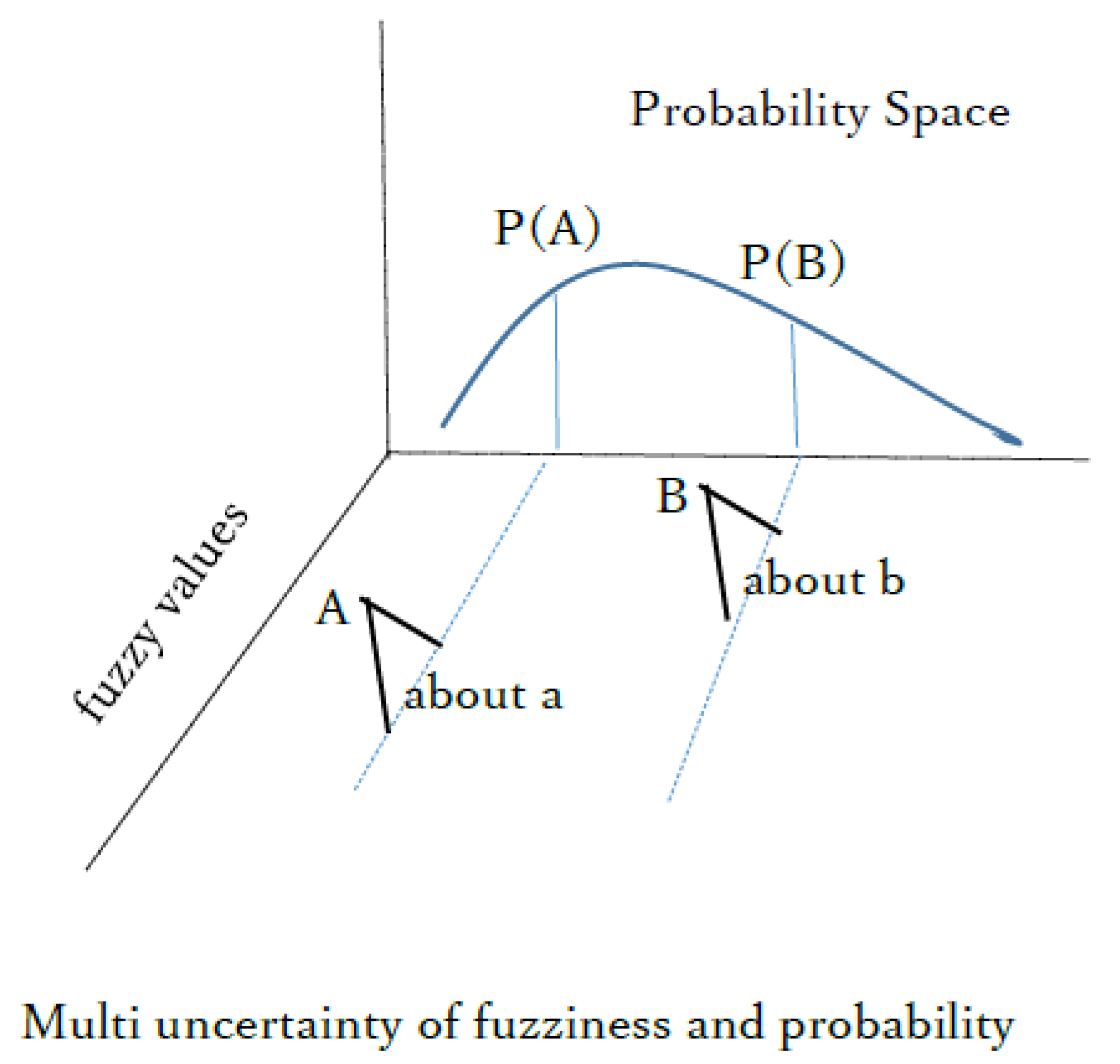
Especially, considering hybrid uncertainty [14], we provide the methodology of fuzzy goal programming (FGP) in hybrid uncertainty. This paper explains the decision making in hybrid uncertainty including fuzziness and randomness. That is, under the situation of fuzzy and randomness hybrid uncertainty, the GP methodology is illustrated.

The paper enables to interpret the decision making in such situation. At the end, we provide a case study of production planning problem to make the method understood clearly.

The remainder of this article is divided into the following sections: There is a brief review of GP and fuzzy programming in Section 2. The FGP is described as the primary technique in Section 3. Section 4 explains the proposed methodology, while Section 5 provides a brief application in production planning. Finally, the conclusions are given in Section 6.

2. Review of Existing Research Works

2.1. Goal Programming (GP)

GP was first used by Charnes, Cooper and Ferguson in 1955 [15], although the actual name first appeared in a 1961 text by Charnes and Cooper. Seminal works by Lee, Ignizio [16], Ignizio and Cavalier [17], and Romero [18] followed. Schniederjans [19] gives in a bibliography of a large number of pre-1995 articles relating to GP, and Jones and Tamiz [20] give an annotated bibliography of a decade in 1990. A recent textbook by Jones and Tamiz [21] gives a comprehensive overview of the state-of-the-art in GP. Mathematics of fuzzy sets has gained popularity in recent years and are employed in a variety of research works to solve a m1ulti-goal mathematical programming problem. It is founded on a concept of contentment. The GP model assists the decision-maker in analyzing many objectives at the same time and selecting the most rewarding action from a set of options. The satisfying notion in GP is to follow decision-makers’ assessment actions in order to achieve a set of stated goals as effectively as feasible [22,23]. The satisfying concept implies that decision-makers will be satisfied if their objectives are attained in the given situation. In decision-making, GPs have proven to be effective. However, GPs face challenges such as determining the right goal values and the lack of decision makers in the modeling process.

A linear goal system with positive and negative changes between each target and goal or aspiration level is known as GP [21,24]. In the specified task, this indicates the most satisfying point for goal accumulation. Based on the concept of “satisfaction”, the GP model’s response is the optimal compromise a decision maker can make [25]. The GP model has two components that can be investigated: set limitations and goal functions.

2.2. Fuzzy Goal Programming (FGP)

FGP is goal programming with fuzzy variables, coefficients, data, criteria, constraints or conditions. For example, a company wants to build a new factory, but it faces many uncertain conditions and environments, has no data as reference, the market is unsteadily, costs are difficult to control, etc. In this case, how do we build a suitable plan to make the new factory profitable? How do we formulate earning target and costs purpose? Like this, we need consider using GP.

The GP model was enhanced using fuzzy set theory [22] to manage uncertainty data, resulting in FGP. The main goal is to improve the ability of FGP to deal with the nature of uncertainty when modeling problems [26,27]. Uncertainties are frequently related to the goal objectives in a case such as a production planning model. However, uncertainties can also come from other elements of the model, such as system constraints. FGP, on the other hand, will only deal with the fuzzy values it has in its model. Other types of uncertainty, such as randomness, that are common in the environment are not handled by the existing FGP. Because fuzziness and randomness are common in real-life events, it is impossible to employ present systematic ways to deal with them, even if they are critical issues that need to be addressed. To tackle the problem of hybrid uncertainty, the fuzzy random approach must be integrated with the existing FGP.

The model’s performance can be influenced by the uncertainty found in the historical data that were used to construct it. Standard analysis is unable to address such data due to the inherent ambiguity. Many methods must be utilized to transform uncertainty into certainty in order to discover the best solution because the facts, goals, or conditions are not always known. The most significant elements to consider are the techniques used and how they are changed. Unlike the traditional GP, the fuzzy model should be deployed first, and the demands of decision makers must be addressed. Although the solution process does not occur simultaneously, the majority of analyses are now employed to deal with fuzzy objectives, constraints, or coefficients. As a result, in order to produce a suitable and adequate model’s solution, this study article considers all of the sections at the same time. From this perspective, developing a fuzzy programming system that can manage many objectives is advantageous. We explore the renewal of the FGP technique to multi-objective problems with hybrid uncertainty, which is motivated by the challenges of such scenarios. Fuzzy random regression [28] is used in this paper to generate a parameter model for modeling program objectives. The translation of fuzzy symbols is demonstrated using the scaled index method to increase the range of unknown numbers to an acceptable level. This is needed to provide flexibility over values as they reflect human decision-making, which tends to be inaccurate. This strategy is accompanied by empirical results that show that the model proposed in the optimization problem satisfies various objectives is ultimately based on the treatment of fuzzy random data that solves the problem of uncertainties in mathematical modeling.

The original GP was developed with objectives, constraints, and goal values that had precise values. However, due to the uncertainty in the scenario, determining the exact value for developing the model is difficult. This occurs when experts are unable to precisely define the value of uncertainty, or when the value is unknown. As a result, fuzzy theory is employed to assist in the conversion of uncertainty into a specific value. Fuzzy values in GP descriptions are used in some ambiguous and imprecise situations. In the GP model, imprecise data show decision makers’ ambiguity or tolerance, as well as expert’s inaccuracies.

To overcome uncertainties in multi-objective decision-making circumstances, FGP combines GP and fuzzy set theory [27]. It’s acceptable to consider that the possible values of the model is features and coefficients are unknown and that the decision maker can offer them, or that these values can be found using historical data or statistical inference. As a result of this exploratory investigation, many varieties of FGP have been studied and widely distributed in the literature [29].

2.3. Fuzzy Multi-Criteria Linear Programming with Uncertainty

This method can be used to meet the following research categories: First, historical data can be used to create an appropriate linear regression model [28] in the event of a situation of difficulty and uncertainty in developing the target. Second, targets (goals) can be determined even if past data is imprecise or unknown. Third, dealing with difficulties that are not specified, such as restrictions or changes in environment.

3. Theoretical Background

3.1. Goal Programming (GP)

The GP model with all deterministic values is written as follows:

$$\begin{array}{cc}\hfill max& {\displaystyle V\left(\mu \right)=\sum _{i=1}^m{\mu }_i}\hfill \\ \\ \hfill \mathrm{subject}\mathrm{to}& {\displaystyle {\mu }_i=\frac{G_i\left(\mathbf{X}\right)-L_i}{g_i-L_i}}\hfill \\ \\ \hfill & \mathbf{A}\mathbf{X}\le \mathbf{b}\hfill \\ \\ \hfill & {\mu }_i\le 1\hfill \\ \\ \hfill & \mathbf{X}\ge \mathbf{0},{\mu }_i\ge 0,\hfill \\ \\ \hfill & i=1,2,\cdots ,m,\hfill \end{array}$$

(1)

The fuzzy accomplishment function $V\left(u\right)$ is used here. In vector, $\mathbf{A}\mathbf{X}\le \mathbf{b}$ denotes the rigid system constraints.

3.2. Fuzzy Goal Programming (FGP)

The problem of FGP is expressed as follows:

$$\begin{array}{c}\mathrm{Find}:\mathbf{x}\hfill \\ \mathrm{to}\mathrm{satisfy}:F_i\left(\mathbf{x}\right)\widetilde{>}{g}_i,i=1,...,n,\hfill \\ \mathrm{subject}\mathrm{to}:\mathbf{Ax}\le \mathbf{b},\mathbf{x}\ge \mathbf{0},\hfill \end{array}$$

(2)

It is worth noting that ∼, such as $\stackrel{\sim }{A}$, is not used to explain a fuzzy set or a fuzzy number because their meaning is obvious in the context.

3.3. Fuzzy Multi-Criteria Linear Programming with Uncertainty

3.3.1. Fuzzy Sets

Definition 1.

Let Pos be a possibility measure defined on the power set Γ of some universe $P(\Gamma )$. ℜ is the set of real numbers. A fuzzy variable defined on Γ is said to be a function $Y:\Gamma \to \Re$. The possibility distribution ${\mu }_Y$ of Y is defined by ${\mu }_Y\left(t\right)=Pos(Y=t)$, $t\in \Re$, which is the possibility of event $(Y=t)$, for fuzzy variable Y. The possibility distribution ${\mu }_Y\left(t\right)$, the possibility, necessity, credibility of event $\{Y\le t\}$ are given, as follows

$$\begin{array}{c}Pos\{Y\le t\}=sup\stackrel{{\mu }_Y}{r\le \tau }\left(t\right)\hfill \\ Nec\{Y\le t\}=1-sup\stackrel{{\mu }_Y}{r\ge \tau }\left(t\right)\hfill \\ {\displaystyle Cr\{Y\le t\}=\frac{1}{2}\left(1+sup\stackrel{{\mu }_Y}{r\le \tau }\left(t\right)-sup\stackrel{{\mu }_Y}{r\ge \tau }\left(t\right)\right)}\hfill \end{array}$$

(3)

The credibility is a self-dual function that is defined as the average of the possibility and necessity metrics $cr(·)=\left(pos\right(·)+nec(·\left)\right)/2$. The credibility criterion aims to develop a technique that combines two extreme examples of possibilities and demands. Possibility is a function that expresses the degree of overlap and is quite optimistic, while being pessimistic and articulating the level of admission is necessity [30]. According to the credibility measure, the expected value of a fuzzy variable is as follows:

Definition 2.

Assume that Y is a fuzzy variable. Expected value of Y is expressed as

$$E[Y]={\int }_0^{\infty }Cr(Y\ge t)dr-{\int }_{-\infty }^{0}Cr(Y\le t)dr$$

(4)

Definition 3.

Let $Y=({\alpha }^l,a,{\alpha }^r)$ be a triangular fuzzy variable with the possibility distribution shown below.

$${\mu }_Y\left(x\right)=\left\{\begin{array}{cc}{\displaystyle \frac{x-a^l}{a-a^l};}\hfill & a^l\le x\le a\hfill \\ \\ {\displaystyle \frac{a^r-x}{a^r-a};}\hfill & a\le x\le a^r\hfill \\ \\ {\displaystyle 0;}\hfill & otherwise\hfill \end{array}\right.$$

(5)

Based on (5), the expected value of Y is determined.

$${\displaystyle E[Y]=\frac{a^l+2a+a^r}{4}}$$

(6)

More theoretical results on fuzzy random variables can be found in Boading Liu [31], Shuming Wang & Watada [14], Jaime Gil-Aluja [32]. Figure 1 shows fuzzy random data. Note that fuzzy numbers occur with probability.

3.3.2. Fuzzy Random Variable

Definition 4.

Assume that the space$(\Omega ,\Sigma ,pr)$is a probability space.$F_v$is a set of fuzzy variables defined on the$(\Gamma ,P(\Gamma ),Pos)$possibility space. A fuzzy random variable is a mapping$X:\Omega \to F_v$such that$Pos\left\{X\right(\omega )\in B\}$is a measurable function of ω for each Borel subset B of ℜ. Let V be a random variable defined on the probability space$(\Omega ,\Sigma ,pr)$, and define$X\left(\omega \right)=\left(V\right(\omega )+2,V(\omega )-2,V(\omega )+6)\tau$, which is a triangular fuzzy variable defined on the possibility space$(\Gamma ,P(\Gamma ),Pos)$for every$\omega \in \Omega$. X is a triangular fuzzy random variable [33].

Definition 5.

Let X be a fuzzy random variable defined on a probability space$(\Omega ,\Sigma ,pr)$. The expected value of X is defined as

$$E[\xi ]=\int [{\int }_0^{\infty }[\underset{0}{\overset{\infty }{inf}}Cr\{Y\ge t\}-\underset{-\infty }{\overset{0}{inf}}Cr\{Y\le t\}dr]$$

(7)

Given that V is a discrete fuzzy random variable that takes $V_1=3$ with probability 0.2 and $V_2=6$ with probability 0.8, the expected value of X is calculated.

Assume V is a discrete fuzzy random variable that has a probability of 0.2 for $V_1=3$ and 0.8 for $V_2=6$. The expected value of X is calculated.

We can deduce the following from Definition 3:

$$\begin{array}{cccc}\hfill X\left(V_1\right)& =& (5,1,9)T,\hfill & pro=0.2,\hfill \\ \hfill X\left(V_2\right)& =& (8,4,12)T,\hfill & pro=0.8,\hfill \end{array}$$

We may then calculate the following using the equation:

$$\begin{array}{c}E\left(X\left(V_1\right)\right)=5,\hfill \\ E\left(X\left(V_2\right)\right)=8,\hfill \\ E\left(X\right)=0.2\times E\left(X\left(V_1\right)\right)+0.8\times E\left(X\left(V_2\right)\right)=7.4\hfill \end{array}$$

Definition 6.

Let X be a fuzzy random variable specified in a probability space with an expected value of e, and $Var[X]=E[(X-e)2]$ be the variance of X. We can deduce the following when the variables are symmetrical triangular fuzzy numbers:

$${\displaystyle Var[X]=\frac{{(X^r-a^l)}^2}{24}}$$

(8)

3.4. Building GP Models with Fuzzy Random Regression

When fuzzy random data are given, we can build a fuzzy random linear regression as in Equation (9). In the Equation (9). Y and X are probabilistic fuzzy numbers, often known as fuzzy random numbers.

$${\displaystyle Y_i=\sum _{j=1}^k{A}_j{X}_{ij}}$$

(9)

Assume the output data are $y_i$, the estimated value is $Y_i$, and the input data are X. To determine the estimated value of $Y_i$, the relationship between the data must be discovered.

$${\displaystyle Y_i=\sum _{j=1}^k{A}_j{X}_{ij}\stackrel{FR}{\supset }{y}_i}$$

(10)

Using $\stackrel{FR}{\supset }$ as a fuzzy random inclusion relationship, the equation is rewritten as follows.

$$\begin{array}{ccc}\hfill {\displaystyle \underset{A_k;k=1\cdots k}{min}}& & {\displaystyle J\left(\mathbf{A}\right)=\sum _{k=1}^k(A_k^r-A_k^l)}\hfill \\ \hfill \mathrm{subject}\mathrm{to}& & A_k^r\ge A_l^{;}\hfill \\ \hfill & & {\displaystyle Y_i=\sum _{j=1}^k{A}_j{X}_{ij}\stackrel{FR}{\supset }{y}_i}\hfill \\ \hfill & & ;i=1,2,\cdots ,n\hfill \\ \hfill & & ;j=1,2,\cdots ,k\hfill \end{array}$$

(11)

The technique of Watada and Wang [34], which is an expected value regression model, is used.

$$\begin{array}{ccc}\hfill {\displaystyle \underset{A_j;j=1\cdots k}{min}}& & {\displaystyle j\left(\mathbf{A}\right)=\sum _{j=1}^k(A_j^r-A_j^l)}\hfill \\ \hfill \mathrm{subject}\mathrm{to}& & A_k^r\ge A_l^{;}\hfill \\ \hfill & & {\displaystyle Y_i=\sum _{j=1}^k{A}_j{X}_{ij}\stackrel{h}{\supset }E\left(y_i\right)}\hfill \\ \hfill & & ;i=1,2,\cdots ,n\hfill \\ \hfill & & ;j=1,2,\cdots ,k\hfill \end{array}$$

(12)

The fuzzy inclusion relation satisfied at level h is combined with the expectation and variance of a fuzzy random variable, as well as the confidence-interval based inclusion relation.

Table 1. Fuzzy random input–output data.

Sample	Output	Input
1	$Y_1$	$X_{11}$	$X_{12}$	⋯	$X_{1j}$	⋯	$X_{1k}$
2	$Y_2$	$X_{21}$	$X_{22}$	⋯	$X_{2j}$	⋯	$X_{2k}$
⋮	⋮	⋮	⋮		⋮		⋮
i	$Y_i$	$X_{i1}$	$X_{i2}$	⋯	$X_{ij}$	⋯	$X_{ik}$
⋮	⋮	⋮	⋮		⋮		⋮
n	$Y_n$	$X_{n1}$	$X_{n2}$	⋯	$X_{nj}$	⋯	$X_{nk}$

is then transformed into

Table 2. Confidence interval based input–output data.

Sample	Output	Input
	$I[e_Y,{\sigma }_Y]$	$I[e_{X_1}.{\sigma }_{X_1}]$	⋯	$I[e_{X_k}{\sigma }_{X_k}]$
1	$I[e_{Y_1},{\sigma }_{Y_1}]$	$I[e_{X_{11}}{\sigma }_{X_{11}}]$	⋯	$I[e_{X_{1k}}{\sigma }_{X_{1k}}]$
⋮	⋮	⋮		$I[e_{X_{1k}}{\sigma }_{X_{1k}}]$
i	$I[e_{Y_i},{\sigma }_{Y_i}]$	$I[e_{X_{i1}}{\sigma }_{X_{i1}}]$	⋯	$I[e_{X_{ik}}{\sigma }_{X_{ik}}]$
⋮	⋮	⋮		$I[e_{X_{1k}}{\sigma }_{X_{1k}}]$
n	$I[e_{Y_n},{\sigma }_{Y_n}]$	$I[e_{X_{n1}}{\sigma }_{X_{n1}}]$	⋯	$I[e_{X_{nk}}{\sigma }_{X_{nk}}]$

.

The confidence interval of a fuzzy random variable is determined by its expectation and variance. For each fuzzy random variable, the one-sigma confidence interval can be represented as one-sigma interval [35,36].

$$I[e_x,{\sigma }_x]\simeq [E\left(x\right)-\sqrt{Var},E\left(x\right)+\sqrt{Var}]$$

(13)

The fuzzy random regression model written as follows:

$$\begin{array}{ccc}\hfill {\displaystyle \underset{A_j;j=1\cdots k}{min}}& & {\displaystyle J\left(\mathbf{A}\right)=\sum _{j=1}^k(A_j^r-A_j^l)}\hfill \\ \hfill \mathrm{subject}\mathrm{to}& & A_j^r\ge A_l^{;}\hfill \\ \hfill & & {\displaystyle Y_i=\sum _{j=1}^k{A}_{j}I[e_x,{\sigma }_x]\stackrel{h}{\supset }I[e_y,{\sigma }_y]}\hfill \\ \hfill & & ;i=1,\cdots ,n\hfill \\ \hfill & & ;j=1,\cdots ,k\hfill \end{array}$$

(14)

The goal equations in this model can be obtained using LINGO.

4. Building Hybrid Uncertainty-GP Model with Scaled Index

The initial method for solving the multi-objective problem discussed in this paper is GP. Because parameter values in objective programming are often difficult to obtain, fuzzy random techniques are used to generate these figures using historical data. However, the uncertainties found in the data to be used to generate the parameter values resulted in a fuzzy random regression approach being chosen to manage these uncertainties. Therefore, the hybrid uncertainty GP model is a GP model derived from fuzzy random regression. To provide an acceptable integer range, an index scale approach was also added in this new model type.

4.1. Constraints Definition

4.1.1. Linear-Fuzzy Constrain Equations

Some of the model’s constraints are not predetermined and can be altered in a variety of ways. Alternatively, one result may have one probability while the other has a different one. Uncertainty must be considered in this instance, and changes must be made during the modeling process. Some fuzzy terms, such as “about” and ”roughly equivalent to”, should be translated into mathematical symbols and numbers. The constraint coefficient is a fuzzy random variable that is set to the expected value in this research. As a result, it is expressed using fuzzy symbols. The constraints model is written as,

$$\begin{array}{ccc}\hfill \mathrm{subject}\mathrm{to}& & {\displaystyle S{\left(\mathbf{X}\right)}_1\sum _{j=1}^k{A}_j{x}_{1j}\prec g_l;}\hfill \\ \hfill & & {\displaystyle S{\left(\mathbf{X}\right)}_2\sum _{j=1}^k{A}_j{x}_{2j}\approx g_2;}\hfill \end{array}$$

(15)

4.1.2. Solving Fuzzy Constraint Equations

1.

Weighting Method

The term “weight” refers to a metric, target, or standard. By comparing them to others, weights are utilised to determine the model’s parameter relative value. The act of assigning different weights to different elements to reflect their relative value is referred to as weighting in the evaluation process. Line supervisors, for example, assess the overall quality of a product based on its appearance, utility, and manufacturing time. Weights should be utilised to connect distinct purposes in linear multi-criteria programming. If the weights are the same, the importance is the same; otherwise, assign them distinct weights.

Equation weights are given to connect three linear equations into one.

$$max{Y}_i=30\%\times Y_1+30\%\times Y_2+30\%\times Y_3$$

(16)

2.

Substitute the precise value $a_k$ for the fuzzy coefficients, which represents the fuzzy random data.

$$\left(\begin{array}{cc}{p}^l& p^r\\ a_k^l& a_k^r\end{array}\right).$$

(17)

3.

Alter the constraints goals $g_i$

Managerial experience is required to obtain random triangular data. For example, we estimate the cost to be roughly 800 dollars. The range of this 800 is continually changing according on the whole supply-demand situation. We can deduce from the statistics and 10-year reference experience that 3 years equals 700 to 800 and 7 years equals 800 to 900. As a result, we show that the likelihood of 800 is 0.3, while the probability of 900 is 0.7. Such situation represents the existence of hybrid uncertainties namely fuzziness and randomness. The expected value can be calculated to provide a coordinated solution to set upper and lower bounds after understanding how to obtain fuzzy random data.

$$\begin{array}{ccc}\hfill {\displaystyle max{Y}_i}& & {\displaystyle J\left(\mathbf{A}\right)=\sum _{j=1}^k{A}_j{X}_{ij}}\hfill \\ \hfill \mathrm{subject}\mathrm{to}& & {\displaystyle S{\left(X\right)}_1:\sum _{j=1}^k{a}_j{X}_{1j}\le E\left(g_1\right);}\hfill \\ \hfill & & {\displaystyle S{\left(X\right)}_2:\sum _{j=1}^k{a}_j{X}_{2j}=E\left(g_2\right);}\hfill \end{array}$$

(18)

4.

Fuzzy Symbols Transformation

The scalable index strategy involves using a scalable number $li$ to raise the range of an unknown integer to an acceptable range. The scalability index was changed to 1 and the range was changed to 9 or 11. Any number in the range [37,38] is appropriate. The wider the range, the higher the scalability index. However, it has a low level of precision. Translate $\prec ,\succ \approx$ to $<,>=.\le ,\ge$

$$\begin{array}{ccc}\hfill {\displaystyle max{Y}_i}& & {\displaystyle Y_i=\sum _{k=1}^k{A}_k{X}_{ik}}\hfill \\ \hfill \mathrm{subject}\mathrm{to}& & {\displaystyle S{\left(X\right)}_1:\sum _{j=1}^k{a}_j{X}_{1j}\le E\left(g_1\right)+l_1;}\hfill \\ \hfill & & {\displaystyle S{\left(X\right)}_2:\sum _{j=1}^k{a}_j{X}_{2j}=E\left(g_2\right)+l_2;}\hfill \end{array}$$

(19)

Boundary can be obtained by calculating Equations (18) and (19).

4.2. Model’s Solution

4.2.1. Max–Min Method

Given two types of linear GP models. The goals are $f\left(x\right)$, the constraint equations are $s\left(x\right)$, and the interval values are $b_i$ and $d_i$.

1. Maximizes the similarity of goals and constraints that are smaller than fuzzy numbers.

Equation (19) is written into the following expression:

$$\begin{array}{ccc}\hfill max& & {\displaystyle f_i\left(\mathbf{x}\right)=\sum _{i=1}^n\sum _{j=1}^k{A}_j{X}_{ij}}\hfill \\ \hfill \mathrm{subject}\mathrm{to}& & S\left(\mathbf{X}\right)=\left\{\begin{array}{c}{a}_{ij}{x}_{ij}\prec [b_i,d_i]\hfill \\ \\ \mathbf{X}\ge \mathbf{0}\hfill \end{array}\right.\hfill \end{array}$$

(20)

$M_G\left(X\right)$ is a membership function of the goal equation, $f\left(x\right)$

$$\begin{array}{c}{\displaystyle M_G\left(\mathbf{x}\right)=\frac{{\displaystyle \sum _{i=1}^n\sum _{j=1}^k{A}_{ij}{x}_{ij}-G_0}}{d_0}}\hfill \\ \\ d_0=G_1-G_2\hfill \end{array}$$

(21)

The maximum value is $G_1$, whereas the minimum value is $G_0$.

$M_G\left(X\right)$ is a membership function of the goal equation, $f\left(x\right)$

$$M_G\left(\mathbf{x}\right)=\left\{\begin{array}{cc}1\hfill & {\displaystyle ;\sum _{i=1}^n\sum _{j=1}^k{a}_j{x}_{ij}\le b_i}\hfill \\ {\displaystyle 1-\frac{{\displaystyle \sum _{i=1}^n\sum _{j=1}^k{a}_i{x}_{ij}-b_i}}{d_i}}\hfill & {\displaystyle ;b_i<\sum _{i=1}^n\sum _{j=1}^k{a}_j{x}_{i,j}\le b_i+d_i}\hfill \\ 0\hfill & {\displaystyle ;\sum _{i=1}^n\sum _{j=1}^k{a}_k{x}_{i,j}\ge b_i+d_i}\hfill \end{array}\right.$$

(22)

To connect $M_G\left(X\right)$ and $M_C\left(X\right)$, the auxiliary variable $lambda$ is used.

$$\begin{array}{ccc}\hfill max& & \lambda \hfill \\ \hfill \mathrm{subject}\mathrm{to}& & \left\{\begin{array}{c}{\displaystyle 1-\frac{{\displaystyle \sum _{i=1}^n\sum _{j=1}^k{a}_i{x}_{ij}-b_i}}{d_i}\ge \lambda }\hfill \\ {\displaystyle \frac{{\displaystyle \sum _{i=1}^n\sum _{j=1}^k{A}_i{X}_{ij}-G_0}}{d_0}\ge \lambda }\hfill \end{array}\right.\hfill \end{array}$$

(23)

2. Minimize goals and constraint equations greater than fuzzy numbers.

$$\begin{array}{ccc}\hfill min& & {\displaystyle f_i\left(\mathbf{x}\right)=\sum _{i=1}^n\sum _{j=1}^k{A}_i{X}_{ij}}\hfill \\ \hfill \mathrm{subject}\mathrm{to}& & s\left(\mathbf{x}\right)=\left\{\begin{array}{c}{a}_i{x}_{ij}\succ [b_i,d_i]\hfill \\ \\ \mathbf{x}\ge \mathbf{0}\hfill \end{array}\right.\hfill \end{array}$$

(24)

$${\displaystyle M_G\left(\mathbf{x}\right)=\frac{{\displaystyle G_0-\sum _{i=1}^n\sum _{j=1}^k{A}_i{X}_{ij}}}{d_0},d_0=G_1-G_0}$$

(25)

The value is $G_1$, whereas the minimum value is $G_0$. The membership function of constraints equations $S\left(x\right)$ is $MC\left(X\right)$.

$$M_G\left(\mathbf{x}\right)=\left\{\begin{array}{cc}1\hfill & {\displaystyle ;\sum _{i=1}^n\sum _{j=1}^k{a}_i{x}_{ij}\ge b_i}\hfill \\ {\displaystyle 1+\frac{{\displaystyle \sum _{i=1}^n\sum _{j=1}^k{a}_i{x}_{ij}-b_i}}{d_i}}\hfill & {\displaystyle ;d_i-d_i\ge \sum _{i=1}^n\sum _{j=1}^k{a}_i{x}_{ij}{x}_{ij}}\hfill \\ \\ 0\hfill & {\displaystyle ;\sum _{i=1}^n\sum _{j=1}^k{a}_i{x}_{ij}{x}_{ij}<d_i-d_i}\hfill \end{array}\right.$$

(26)

The auxiliary variable $\lambda$ is used to connect $M_G\left(X\right)$ and $M_C\left(X\right)$.

$$\begin{array}{ccc}\hfill max& & \lambda \hfill \\ \hfill \mathrm{subject}\mathrm{to}& & \left\{\begin{array}{c}{\displaystyle 1+\sum _{i=1}^n\sum _{j=1}^k{a}_i{x}_{ij}\ge \lambda }\hfill \\ {\displaystyle \frac{{\displaystyle G_0-\sum _{i=1}^n\sum _{j=1}^k{A}_i{X}_{ij}}}{d_1}\ge \lambda }\hfill \end{array}\right.\hfill \end{array}$$

(27)

3. Maximize and minimize goals and constraint equations have $\prec ,\succ$ at the same time.

$$\begin{array}{cc}\mathrm{Evaluation}\hfill & \left\{\begin{array}{c}{\displaystyle max{f}_i\left(\mathbf{x}\right)=\sum _{i=1}^n\sum _{j=1}^k{A}_{i,j}{X}_{ij}}\hfill \\ {\displaystyle min{f}_i\left(\mathbf{x}\right)=\sum _{i=1}^n\sum _{j=1}^k{A}_{i,j}{X}_{ij}}\hfill \end{array}\right.\hfill \\ \mathrm{subject}\mathrm{to}\hfill & S\left(\mathbf{x}\right)=\left\{\begin{array}{c}{a}_{i,j}{x}_{ij}\succ [b_i,d_i]\hfill \\ a_{i,j}{x}_{ij}\prec [b_i,d_i]\hfill \\ \mathbf{x}\ge \mathbf{0}\hfill \end{array}\right.\hfill \end{array}$$

(28)

Introduce the auxiliary variable $\lambda$ to connect $M_G\left(X\right)$ and $M_C\left(X\right)$.

$$\begin{array}{cc}max\hfill & \lambda \hfill \\ \mathrm{subject}\mathrm{to}\hfill & \left\{\begin{array}{c}{\displaystyle 1-\frac{{\displaystyle \sum _{i=1}^n\sum _{j=1}^k{a}_i{x}_{ij}-b_i}}{d_i}\ge \lambda }\hfill \\ {\displaystyle 1+\frac{{\displaystyle \sum _{i=1}^n\sum _{j=1}^k{a}_i{x}_{ij}-b_i}}{d_i}\ge \lambda }\hfill \\ {\displaystyle \frac{{\displaystyle \sum _{i=1}^n\sum _{j=1}^k{A}_i{X}_{ij}-G_0}}{d_0}\ge \lambda }\hfill \\ {\displaystyle G_0-\frac{{\displaystyle \sum _{i=1}^n\sum _{j=1}^k{A}_i{X}_{ij}}}{d_0}\ge \lambda }\hfill \end{array}\right.\hfill \end{array}$$

(29)

4.2.2. Constructing Membership Function

1. Goals’ membership function The solution boundary is derived using Equations (28) and (29). So, the difference is $d_0=f_1-f_0$,

$$\begin{array}{cc}\hfill max& \lambda \hfill \\ \hfill \mathrm{subject}\mathrm{to}& \mu \left(Y_i\right)=\left\{\begin{array}{cc}1\hfill & :Y_i\le f_0+d_0\hfill \\ \\ {\displaystyle \frac{1}{d_0}[Y_i-f_0]}\hfill & ;f_0+d_0<Y_i\le f_0:d_0\hfill \\ \\ 0\hfill & ;Y_i>f_0\hfill \end{array}\right.\hfill \end{array}$$

(30)

2. Constraints’ membership function

$$\mu \left(Y_i\right)=\left\{\begin{array}{cc}1\hfill & :S\left(X\right)\le E\left(g_i\right)\hfill \\ {\displaystyle 1-\frac{1}{l_i}[S\left(X\right)-E\left(g_i\right)]}\hfill & ;E\left(g_i\right)<S\left(X\right)\le E\left(g_i\right)+l_i\hfill \\ 0\hfill & ;S\left(X\right)>E\left(g_i\right)+l_i\hfill \end{array}\right.$$

(31)

$l_i$ is scalable index, $s\left(x\right)$ are constraints’ equations, $E\left(g_i\right)$ is expected value of $g_i$.

3. Connect the goals and constraints of the membership function

By referring to the max–min approach, an auxiliary variable $\lambda$ is introduced to obtain a new equivalent model.

$$\begin{array}{cc}max\hfill & \lambda \hfill \\ \mathrm{subject}\mathrm{to}\hfill & \left\{\begin{array}{c}{\displaystyle 1-\frac{1}{l_i}[S\left(X\right)-E\left(g_i\right)]\ge \lambda }\hfill \\ {\displaystyle \frac{1}{d_0}[Y_i-f_0]\ge \lambda }\hfill \end{array}\right.\hfill \end{array}$$

(32)

The proposed method’s process flow is summarized as follows:

(1)

To generate goal equations, a regression model was utilised to obtain coefficients by using series fuzzy random data.

(2)

Build constraints equations which includes the fuzzy random data, fuzzy symbols, fuzzy goal values.

(3)

Transform fuzzy random data by calculating the expectation. By adding tolerance to goal values, convert fuzzy symbols like $\prec ,\succ \approx$ to $<,>,=.$

(4)

Get the boundary numbers o and give the goal equations the same weights when the importance of the goals is equal. The weights are different if they are not.

(5)

The max–min and scalable index approaches were used to formulate the membership function.

The technique outlined above is sufficient for creating a production planning model that takes into account hybrid uncertainty.

5. Application to Production Planning Assessment

A company wants to build a new plant, but it lacks precise historical data and rely on data from previous facilities as a reference. How can a management construct a fair time, production, and labour cost plan while also satisfying the expectations of other managers in this scenario?

Table 3. Original product quantities, working time, price, and cost data.

Year	Product Quantities		Working Time	Price A and B	Cost A and B
	A	B	Process 1 and 2	Per Dozen	Per Dozen
	${\mathit{X}}_{\mathbf{1}}$	${\mathit{X}}_{\mathbf{2}}$	${\mathit{Y}}_{\mathbf{1}}(\times {\mathbf{10}}^{\mathbf{3}})$	${\mathit{Y}}_{\mathbf{2}}(\times {\mathbf{10}}^{\mathbf{4}})$	${\mathit{Y}}_{\mathbf{3}}(\times {\mathbf{10}}^{\mathbf{4}})$
1	$(\stackrel{0.5}{60},\stackrel{0.5}{70})$	$(\stackrel{0.5}{50},\stackrel{0.5}{55})$	$(\stackrel{0.1}{1.50},\stackrel{0.9}{1.55})$	$(\stackrel{0.1}{8.00},\stackrel{0.9}{8.50})$	$(\stackrel{0.5}{2.00},\stackrel{0.5}{2.50})$
2	$(\stackrel{0.4}{70},\stackrel{0.6}{75})$	$(\stackrel{0.5}{60},\stackrel{0.5}{75})$	$(\stackrel{0.1}{1.60},\stackrel{0.9}{1.75})$	$(\stackrel{0.1}{8.50},\stackrel{0.9}{9.00})$	$(\stackrel{0.5}{2.00},\stackrel{0.5}{2.80})$
3	$(\stackrel{0.3}{80},\stackrel{0.7}{95})$	$(\stackrel{0.6}{85},\stackrel{0.4}{95})$	$(\stackrel{0.6}{1.70},\stackrel{0.4}{1.75})$	$(\stackrel{0.2}{9.50},\stackrel{0.8}{9.80})$	$(\stackrel{0.6}{2.50},\stackrel{0.4}{2.80})$
4	$(\stackrel{0.3}{60},\stackrel{0.7}{70})$	$(\stackrel{0.4}{85},\stackrel{0.6}{95})$	$(\stackrel{0.6}{1.80},\stackrel{0.4}{1.85})$	$(\stackrel{0.2}{9.50},\stackrel{08}{11.00})$	$(\stackrel{0.6}{2.50},\stackrel{0.4}{3.00})$
5	$(\stackrel{0.5}{90},\stackrel{0.5}{115})$	$(\stackrel{0.2}{75},\stackrel{0.8}{90})$	$(\stackrel{0.3}{1.80},\stackrel{0.7}{1.95})$	$(\stackrel{0.3}{11.00},\stackrel{07}{11.50})$	$(\stackrel{0.8}{2.55},\stackrel{0.2}{3.00})$
6	$(\stackrel{0.7}{130},\stackrel{0.3}{145})$	$(\stackrel{0.2}{95},\stackrel{0.8}{110})$	$(\stackrel{0.3}{1.90},\stackrel{0.7}{1.95})$	$(\stackrel{0.1}{11.00},\stackrel{09}{12.00})$	$(\stackrel{0.1}{2.55},\stackrel{0.9}{3.00})$
7	$(\stackrel{0.7}{150},\stackrel{0.3}{165})$	$(\stackrel{0.1}{120},\stackrel{0.9}{130})$	$(\stackrel{0.8}{2.00},\stackrel{0.2}{2.15})$	$(\stackrel{0.1}{12.00},\stackrel{09}{12.50})$	$(\stackrel{0.2}{3.05},\stackrel{0.8}{3.10})$
8	$(\stackrel{0.6}{135},\stackrel{0.4}{160})$	$(\stackrel{0.1}{140},\stackrel{0.9}{160})$	$(\stackrel{0.8}{2.00},\stackrel{0.2}{2.25})$	$(\stackrel{0.1}{1.200},\stackrel{09}{13.00})$	$(\stackrel{0.5}{35.5},\stackrel{0.5}{3.80})$
9	$(\stackrel{0.5}{160},\stackrel{0.5}{180})$	$(\stackrel{0.3}{150},\stackrel{0.7}{170})$	$(\stackrel{0.5}{2.10},\stackrel{0.5}{2.25})$	$(\stackrel{0.5}{12.50},\stackrel{05}{13.50})$	$(\stackrel{0.5}{3.65},\stackrel{0.5}{4.00})$
10	$(\stackrel{0.5}{185},\stackrel{0.5}{215})$	$(\stackrel{0.5}{160},\stackrel{0.5}{180})$	$(\stackrel{0.1}{22.0},\stackrel{0.9}{22.5})$	$(\stackrel{0.7}{12.50},\stackrel{03}{14.50})$	$(\stackrel{0.4}{40.5},\stackrel{0.6}{43.0})$
11	$(\stackrel{0.5}{215},\stackrel{0.5}{235})$	$(\stackrel{0.5}{180},\stackrel{0.5}{190})$	$(\stackrel{0.1}{2.30},\stackrel{0.9}{2.35})$	$(\stackrel{0.2}{13.50},\stackrel{08}{14.50})$	$(\stackrel{0.2}{4.25},\stackrel{0.8}{4.50})$

Note: The above rondom values follow the Definition 17.

provides information on product quantities, working time, price, and cost from the other factories from the first to the eleventh year.

Table 4. Production Constraints.

	Product
Product quantities	$X_1$ (about)	$X_2$ (about)
Price (per dozen)	$9.00(\times {10}^4)$	$6.00(\times {10}^4)$
Cost (per dozen)	$3.00(\times {10}^4)$	$2.00(\times {10}^4)$
Process 1 time (per dozen)	2	3
Process 2 time (per dozen)	6	3

shows the capacity and constraints of production. We need to identify some procedures to formulate a production planning model using the regression model. Working time goals, pricing goals, and cost targets for the 12th year are all involved. The constraint equation is then built. Fuzzy coefficients, fuzzy symbols, and constraint fuzzy objectives are all examples of values that need to be transformed to certain integers. Following that, the membership function was created using the max–min and scalable index methods. Finally, solve the equation.

Manager wants to get some objectives based on reference data in Table 3 and Table 4.

(1)

maximize reveues as much as possible over 1800 m

(2)

produce $x_1$ at least 150

(3)

produce $x_2$ at least 100

(4)

Make the working time of 1.2 as close to the maximum limit time as possible.

5.1. Construction of Goal Equations

Rules or relationships between data should be obtained using regression models to construct goal equations. Coefficients are relationships in linear regression models. As a result, obtaining coefficients is a way of setting targets. The linear regression model is shown in the followings:

$$\begin{array}{c}{Y}_1=A_{11}{X}_1+A_{12}{X}_2\hfill \\ Y_2=A_{21}{X}_1+A_{22}{X}_2\hfill \\ Y_3=A_{31}{X}_1+A_{32}{X}_2\hfill \end{array}$$

(33)

The expectation of Table 3 and Table 4 are calculated from Definitions 3 and 4,

5.2. Example

For instance, if we take a fuzzy random number like $a_1=(0.3/2,0.7/7)$ from the distribution, and fuzzy random variable takes $(0.3/(0.3/(4,0,8)),0.7/(0.5/(9,5,13))$, the expected value $a_1$ can be calculated as follows:

$${\displaystyle E\left(a_1\right)=0.3\times \frac{0+2\times 4+8}{4}+0.7\times \frac{5+2\times 9+13}{4}=7.5}$$

Variance value of

Table 5. Expected values.

Year	Product Quantities		Working Time	Price A and B	Cost A and B
	A	B	Process 1 and 2	Per Dozen	Per Dozen
	$\mathit{E}\left({\mathit{X}}_{\mathbf{1}}\right)\left({\mathbf{10}}^{\mathbf{2}}\right)$$\mathit{E}\left({\mathit{X}}_{\mathbf{2}}\right)\left({\mathbf{10}}^{\mathbf{2}}\right)$		$\mathit{E}\left({\mathit{Y}}_{\mathbf{1}}\right)\left({\mathbf{10}}^{\mathbf{5}}\right)$	$\mathit{E}\left({\mathit{Y}}_{\mathbf{2}}\right)\left({\mathbf{10}}^{\mathbf{2}}\right)$	$\mathit{E}\left({\mathit{Y}}_{\mathbf{3}}\right)\left({\mathbf{10}}^{\mathbf{2}}\right)$
1	7.500	6.25	1.625	8.55	2.35
2	8.300	77.5	1.590	9.05	2.50
3	10.05	79.0	1.820	9.84	2.72
4	8.300	101	1.920	10.80	2.80
5	11.25	97.0	2.005	11.50	2.74
6	14.45	117	2.035	12.00	3.01
7	16.45	139	2.130	12.55	3.19
8	15.50	168	2.150	12.60	3.775
9	18.50	174	2.275	13.10	3.925
10	21.00	175	2.345	13.20	4.30
11	23.50	195	2.445	14.40	4.55

Note: The interval of expected values and variance per year are obtained as Table 6, Table 7 and Table 8, from function (13).

can be calculated based on functions (13) and (14).

The coefficients can be obtained using Equation (14) and LINGO. The $Y_1$ calculation method is as follows, and the $Y_2$ and $Y_3$ calculation processes are the same.

$$\begin{array}{cc}\hfill min& J\left(\mathbf{A}\right)=A_{i1}^r-A_{i1}^l+A_{i2}^r-A_{i2}^l\hfill \\ \hfill \mathrm{subject}\mathrm{to}& A_{i1}^l\times I_{X_1}^l+A_{i2}^l\times I+{X_2}^l\le I_{Y_1}^l\hfill \\ \hfill & A_{i1}^r\times I_{X_1}^r+A_{i2}^r\times I+{X_2}^r\ge I_{Y_1}^r\hfill \end{array}$$

$$\left\{\begin{array}{cc}\hfill & 7.296\times {10}^1\times A_{11}^l+6.149\times {10}^1\times A_{12}^l\le 1.615\times {10}^3\hfill \\ \hfill & 8.198\times {10}^1\times A_{11}^l+7.444\times {10}^1\times A_{12}^l\le 1.540\times {10}^3\hfill \\ \hfill & 9.744\times {10}^1\times A_{11}^l+7.696\times {10}^1\times A_{12}^l\le 1.810\times {10}^3\hfill \\ \hfill & 8.096\times {10}^1\times A_{11}^l+9.896\times {10}^1\times A_{12}^l\le 1.910\times {10}^3\hfill \\ \hfill & 1.4\times {10}^3\times A_{11}^l+9.394\times {10}^1\times A_{12}^l\le 1.974\times {10}^3\hfill \\ \hfill & 1.414\times {10}^2\times A_{11}^l+1.139\times {10}^2\times A_{12}^l\le 2.025\times {10}^3\hfill \\ \hfill & 161.4\times {10}^2\times A_{11}^l+1.370\times {10}^2\times A_{12}^l\le 2.099\times {10}^3\hfill \\ \hfill & 151.9\times {10}^2\times A_{11}^l+1.639\times {10}^2\times A_{12}^{.}l\le 2.099\times {10}^3\hfill \\ \hfill & 180.9\times {10}^2\times A_{11}^l+1.699\times {10}^2\times A_{12}^{.}l\le 2.244\times {10}^3\hfill \\ \hfill & 203.9\times {10}^2\times A_{11}^l+1.709\times {10}^2\times A_{12}^{.}l\le 2.335\times {10}^3\hfill \\ \hfill & 230.9\times {10}^2\times A_{11}^l+1.930\times {10}^2\times A_{12}^l\le 2.435\times {10}^3\hfill \\ \\ \hfill & 7.704\times {10}^2\times A_{11}^r+6.149\times {10}^1\times A_{12}^r\ge 1.635\times {10}^3\hfill \\ \hfill & 0.840\times {10}^2\times A_{11}^r+8.056\times {10}^1\times A_{12}^r\ge 1.626\times {10}^2\hfill \\ \hfill & 1.036\times {10}^2\times A_{11}^r+8.104\times {10}^1\times A_{12}^r\ge 1.830\times {10}^3\hfill \\ \hfill & 8.650\times {10}^2\times A_{11}^r+1.030\times {10}^2\times A_{12}^r\ge 1.930\times {10}^3\hfill \\ \hfill & 1.176\times {10}^2\times A_{11}^r+1.001\times {10}^2\times A_{12}^r\ge 2.036\times {10}^3\hfill \\ \hfill & 1.476\times {10}^2\times A_{11}^r+1.201\times {10}^2\times A_{12}^r\ge 2.045\times 10{.}^3\hfill \\ \hfill & 1.676\times {10}^2\times A_{11}^r+1.410\times {10}^2\times A_{12}^r\ge 2.161\times {10}^3\hfill \\ \hfill & 1.581\times {10}^2\times A_{11}^r+1..721\times {10}^2\times A_{12}^r\ge 2.201\times {10}^3\hfill \\ \hfill & 1.891\times {10}^2\times A_{11}^r+1.781\times {10}^2\times A_{12}^r\ge 2.306\times {10}^3\hfill \\ \hfill & 2.161\times {10}^2\times A_{11}^r+179.08\times {10}^2\times A_{12}^r\ge 2.335\times {10}^3\hfill \\ \hfill & 2.391\times {10}^2\times A_{11}^r+197.04\times {10}^2\times A_{12}^r\ge 2.455\times {10}^3\hfill \end{array}\right.$$

From above, the coefficients are obtained.

To construct the three goals, we use the average number as the final value.

$$\begin{array}{c}{Y}_1=9.05X_1+8.21X_2\hfill \\ Y_2=366.74X_1+604.1X_2\hfill \\ Y_3=134.68X_1+143.06X_2\hfill \end{array}$$

(34)

5.3. Formulation of Constraints’ Equations

Table 10 is derived from

Table 9. Coefficients’ values.

${\mathit{A}}_{\mathbf{11}}$		Average Value	${\mathit{A}}_{\mathbf{12}}$		Average Value
$A_{11}^L$	$A_{11}^R$	${\displaystyle \frac{(A_{11}^L+A_{11}^R)}{2}}$	$A_{12}^L$	$A_{12}^R$	${\displaystyle \frac{(A_{12}^L+A_{12}^R)}{2}}$
0.1967	18.09	9.05	12.62	3.803	8.21
${\mathit{A}}_{\mathbf{21}}$			${\mathit{A}}_{\mathbf{22}}$
$A_{21}^L$	$A_{21}^R$	${\displaystyle \frac{(A_{21}^L+A_{21}^R)}{2}}$	$A_{22}^L$	$A_{22}^R$	${\displaystyle \frac{(A_{22}^L+A_{22}^R)}{2}}$
0.1967	733.5	366.7	735.7	472.5	604.1
${\mathit{A}}_{\mathbf{31}}$		Average Value	${\mathit{A}}_{\mathbf{32}}$		Average Value
$A_{31}^L$	$A_{31}^R$	${\displaystyle \frac{(A_{31}^L+A_{31}^R)}{2}}$	$A_{32}^L$	$A_{32}^R$	${\displaystyle \frac{(A_{32}^L+A_{32}^R)}{2}}$
0.6474	269.4	134.7	59.34	226.8	143.1

. The data are obtained based on references and past experience. $[8.500\times {10}^4,9.500\times {10}^4;0.3,0.7]$ indicates that $x_1$’s price is in the interval of $8.500\times {10}^4$ with probability $0.3$ to $9.500\times {10}^4$ with probability $0.7$. Using the Definitions 3 and 4, the expected values are acquired.

Manager wants their requirements to be met based on the reference data in

Table 10. Production constraints.

	Product
	$A$	$B$
Product quantities	$X_1$	$X_2$
Price (per dozen)	$[8.500\times {10}^4,9.500\times {10}^4;0.3,0.7]$	$[5.800\times {10}^4,6.200\times {10}^4;0.2,0.8]$
Cost (per dozen)	$[2.600\times {10}^4,3.600\times {10}^4,0.5,0.5]$	$[1.800\times {10}^4,2.200\times {10}^4;0.7,0.3]$
Process 1 time (per dozen)	$[1.8,2.2;0.4,0.6]$	$[2.7,3.3;0.6,0.4]$
Process 2 time (per dozen)	$[5.5,6.5;0.3,0.7]$	$[2.8,3.2;0.9,0.1]$

and

Table 11. Production constraints expected value.

	Product
	$A$	$B$
Product quantities	$X_1$	$X_2$
Price (per dozen)	$9.200\times {10}^4$	$96.12\times {10}^4$
Cost (per dozen)	$3.100\times {10}^4$	$1.920\times {10}^4$
Process 1 time (per dozen)	$2.04$	$2.94$
Process 2 time (per dozen)	$6.2$	$2.84$

.

(1)

maximize revenues as much as possible over 1800 m.

(2)

produce product $x_1$ at least 150.

(3)

produceproduct $x_2$ at least 100.

(4)

Make the working time of products 1 and 2 as near to the maximum time restriction as possible.

The needs of managers are presented in fuzzy numbers, which must be converted to fuzzy random data.

(1)

maximize revenues are [$1.700\times {10}^7,1.900\times {10}^7$; 0.5, 0.5]

(2)

produce product $x_1$ is [140, 160; 0.3, 0.7]

(3)

produce product $x_2$ is [80,120; 0.5, 0.5]

(4)

make working time of products 1 and 2 as [800,1000; 0.5,0.5] and [1600,2000; 0.4,0.6]

Five constraints equations are constructed based on the production constraints and the manager’s requirements. The expression of numbers and symbols is in fuzzy.

$$S_i\left(\mathbf{x}\right)\left\{\begin{array}{c}{g}_1:\mathrm{about}2\times X_1+\mathrm{about}3\times X_2\prec \mathrm{about}900\hfill \\ g_5:\mathrm{about}6\times X_1+\mathrm{about}3\times X_2\prec \mathrm{about}1800\hfill \end{array}\right.$$

(35)

After that, the numbers are converted to expected values, and the formulae are employed to calculate the lower limits.

$$S_i\left(\mathbf{x}\right)\left\{\begin{array}{c}{g}_1:6.100\times {10}^4\times X_1+4.200\times {10}^4\times X_2\succ 1.800\times {10}^7\hfill \\ g_2:X_1\succ 154\hfill \\ g_3:X_2\succ 100\hfill \\ g_4:2.04\times X_1+2.94\times X_2\prec 900\hfill \\ g_5:6.2\times X_1+2.84\times X_2\prec 1840\hfill \end{array}\right.$$

(36)

To alleviate the uncertainty of fuzzy symbols, scalable indicies are introduced (undetermined relation). We give scalable index 1,000,000 to $g_1$, 20 to $g_2$, 20 to $g_3$, 100 to $g_4$, and 200 to $g_5$. As a result, the following are the new constraints equations:

$$S_i\left(\mathbf{x}\right)\left\{\begin{array}{c}{g}_1:61000\times X_1+42000\times X_2\ge 19000000\hfill \\ g_2:X_1\ge 174\hfill \\ g_3:X_2\ge 120\hfill \\ g_4:2.04\times X_1+2.94\times X_2\le 1000\hfill \\ g_5:6.2\times X_1+2.84\times X_2\le 2040\hfill \end{array}\right.$$

(37)

These equations are to be regarded as upper bounds in this case [37,38].

5.4. Solution of the Multi-Criteria Linear Goal Models

Three goal models are built in the following:

$$\begin{array}{c}{\displaystyle Y_1=\underset{X_1,X2}{min}9.05\times X_1+8.21\times X_2;}\hfill \\ \\ {\displaystyle Y_2=\underset{X_1,X2}{max}3.6674\times {10}^2\times X_1+6.041\times {10}^2{X}_2;}\hfill \\ \\ {\displaystyle Y_3=\underset{X_1,X2}{min}1.3468\times {10}^2\times X_1+1.4306\times {10}^2\times X_2;}\hfill \end{array}$$

(38)

To meet all of the tree goals at the same time, we assign the same weights of 0.333 and merge them into a single equation.

$$\begin{array}{cc}\hfill {\displaystyle \underset{X_1,X2}{max}}& 0.333\times (9.05\times X_1+8.21\times X_2)+0.333\times (3.667\times {10}^2\times X_1+6.041\times {10}^2\times X_2)\hfill \\ \\ \hfill & =-0.333\times (1.347\times {10}^2\times X_1+1.431\times {10}^2\times X_2);\hfill \end{array}$$

(39)

After linking the objective and constraint equations, the upper and lower limits are obtained.

$$\begin{array}{ccc}\hfill max& & \{-0.333\times (9.05\times X_1+8.21\times X_2)+0.333\times (366.74\times X_1+604.1\times X_2)\hfill \\ \hfill & & -0.333\times (134.7\times X_1+143.1\times X_2)\};\hfill \\ \hfill \mathrm{Subject}\mathrm{to}& & 6.{100}^4\times x_1+4.200\times {10}^4\times x_{\ge }1.800\times {10}^7;\hfill \\ \hfill & & x_1\ge 1.540\times {10}^2;\hfill \\ \hfill & & x_2\ge 1.000\times {10}^2;\hfill \\ \hfill & & 2.04\times x_1+2.94\times x_2\le 9.000\times {10}^2;\hfill \\ \hfill & & 6.2\times x_1+2.84\times x_2\le 1.840\times {10}^3;\hfill \end{array}$$

(40)

$$\begin{array}{cc}\hfill Y_1& {\displaystyle =\underset{X_1,X_2}{min}9.05\times X_1+8.21\times X_2;}\hfill \\ \\ \hfill Y_2& {\displaystyle =\underset{X_1,X_2}{max}3.6674\times {10}^2\times X_1+6.041\times {10}^2\times X_2;}\hfill \\ \\ \hfill Y_3& {\displaystyle =\underset{X_1,X_2}{min}1.3468\times {10}^2\times X_1+1.4306\times {10}^2\times X_2;}\hfill \end{array}$$

(41)

$$\begin{array}{ccc}\hfill {\displaystyle \underset{X_1,X_2}{max}}& & \{-0.333\times (9.05\times X_1+8.21\times X_2)+0.333\times (366.7\times X_1+604.1\times X_2)\hfill \\ \hfill & & -0.333\times (134.68\times X_1+143.06\times X_2);\}\hfill \\ \hfill \mathrm{Subject}\mathrm{to}& & 6.1000\times {10}^4\times x_1+4.2000\times {10}^4\times x_2\ge 1.9000\times {10}^7;\hfill \\ \hfill & & x_1\ge 174;\hfill \\ \hfill & & x_2\ge 120;\hfill \\ \hfill & & 2.04\times x_1+2.94\times x_2\le 1.000\times {10}^3;\hfill \\ \hfill & & 6.2\times x_1+2.84\times x_2\le 2.040\times {10}^3;\hfill \end{array}$$

(42)

By calculation, the upper and lower limits are

$$\begin{array}{cccc}\hfill (X_1& =& 1.6144\times {10}^2,\hfill & X_2=1.9411\times {10}^2)\hfill \\ \hfill (X_1& =& 1.7400\times {10}^2,\hfill & X_2=2.1940\times {10}^2)\hfill \\ \hfill Y_1& =& [3.0548,\times {10}^3,\hfill & 3.3760\times {10}^3]\hfill \\ \hfill Y_2& =& [1.7647\times {10}^5,\hfill & 1.9635\times {10}^5]\hfill \\ \hfill Y_3& =& [4.9512\times {10}^4,\hfill & 5.4822\times {10}^4]\hfill \end{array}$$

The fuzziness are $d_1=321.29,d_2=19883.94,d_3=5309.56$.

The following equation is built by utilizing max–min method and Equations (20) and (21).

$${\mu }_{G_i}\left(\mathbf{x}\right)=\left\{\begin{array}{c}{\displaystyle \frac{1}{3.2129\times {10}^2}[30.547\times {10}^3-f\left(Y_1\right)]}\hfill \\ \\ {\displaystyle \frac{1}{1.9883\times {10}^4}[f\left(Y_2\right)-1.7647\times {10}^5]}\hfill \\ \\ {\displaystyle \frac{1}{5.3096\times {10}^3}[4.9512\times {10}^4-f\left(Y_1\right)]}\hfill \end{array}\right.$$

(43)

By combining the two membership functions and adding the auxiliary variable $\lambda$, a new equivalent model is created.

$$\begin{array}{cc}\hfill max& \lambda \hfill \\ \hfill \mathrm{subject}\mathrm{to}& \left\{\begin{array}{c}{\displaystyle \frac{1}{1.3213\times {10}^2}[3.0547\times {10}^3-f\left(Y_1\right)]\ge \lambda }\hfill \\ \\ {\displaystyle \frac{1}{1.9884\times {10}^4}[f\left(Y_2\right)-1.1765\times {10}^5]\ge \lambda }\hfill \\ \\ {\displaystyle \frac{1}{5.3100\times {10}^3}[4.9512\times {10}^4-f\left(Y_1\right)]\ge \lambda }\hfill \\ \\ {\displaystyle 1+\frac{1}{1.000\times {10}^6}[s_1\left(x\right)-1.8000\times {10}^7]\ge \lambda }\hfill \\ \\ {\displaystyle 1+\frac{1}{20}[s_2\left(x\right)-154]\ge \lambda }\hfill \\ \\ {\displaystyle 1+\frac{1}{20}[s_3\left(x\right)-100]\ge \lambda }\hfill \\ \\ {\displaystyle 1+\frac{1}{100}[s_4\left(x\right)-100]\ge \lambda }\hfill \\ \\ {\displaystyle 1+\frac{1}{200}[s_5\left(x\right)-100]\ge \lambda }\hfill \end{array}\right.\hfill \end{array}$$

(44)

Through calculation, $x_1=1.446\times {10}^2,x_2=2.218\times {10}^2$ and $\lambda =0.5299$ are obtained. The values are then used in the following equations:

$$\begin{array}{c}{Y}_1=9.05\times X_1+8.21\times X_2;\hfill \\ Y_2=3.667\times {10}^2\times X_1+6.041\times {10}^2\times X_2;\hfill \\ Y_3=1.347\times {10}^2\times X_1+1.431\times {10}^2\times X_2,\hfill \\ Y_1=3.129\times {10}^2,Y_2=1.8701\times {10}^5,Y_3=5.1203\times {10}^4,\hfill \end{array}$$

The upper and lower limits are obtained as

$$\begin{array}{c}Y1=[3.0547\times {10}^3,3.3760\times {10}^3],\hfill \\ Y2=[1.7647\times {10}^5,1.9635\times {10}^5],\hfill \\ Y3=[4.9512\times {10}^4,5.4822]\times {10}^4.\hfill \end{array}$$

These results are acceptable.

6. Conclusions

The production planning process in industry involves a variety of responsibilities and real situations. It requires the management to make judgments and decisions that are in the best interests of the factory or business. As a result, the mathematical solution approach has been found to be beneficial in assisting in the creation of a solution. The FGP approach has been discovered to be capable of addressing the three categories of challenges listed below from two perspectives. To begin, if a manager faces a situation in which he or she is unsure how to achieve a realistic goal, an acceptable linear regression model can be developed using historical data to generate a target problem model. Second, even if earlier data failed to precisely predict the current condition, which should not be surprising, mathematical models can still be produced utilizing the uncertainty technique while accounting for this uncertainty. Third, some unidentified issues, such as constraints, can be solved where the situation is not improving and can be altered. The data utilized, on the other hand, have an impact on the model’s accuracy. Because the model parameters are obtained from the raw data, this is the case. There are numerous sources of uncertainty, including inaccuracies, which can affect the accuracy of the data and forecast findings. As a result, for data with uncertainty characteristics, additional data processing approaches are required.

This research has provided the GP model to deal with hybrid uncertainty, hybrid uncertainty, interval fuzziness, type 2 fuzziness. This paper concentrated only on fuzzy multi-criterion decision making by means of fuzzy regression method. The method enables us to treat such uncertainty by using fuzzy numbers. Especially, using the application to ploduction planning, we provided the assessment method of uncertainty. Repeatedly, we emphasize the points we provided in the paper that considering hybrid uncertainty [14], we provided the methodology of FGP in hybrid uncertainty. This paper explained the decision making in hybrid uncertainty including fuzziness and randomness.

The paper enabled us to interpret the decision making in such situation using the case study of production planning problem.

Future Research

We have discussed hybrid uncertainty-GP model. Such hybrid uncertainty comes from fuzzy sets, interval fuzzy sets, type 2fuzzy sets as well as intuitionistic fuzzy sets. tevarious uncertainties such as interval fuzzy sets, type 2 fuzzy sets, intuitionistic fuzzy sets. Inorder to deal with such uncertainty, we can employ rough sets [39], support vector machine [40,41,42,43,44], neural networks [45,46], as well as deep learning. We proposed the decision making under hybrid uncertainty by means of fuzzy random GP. Regarding decision making we may employ a rough set approach [47,48] which has capability to obtain decision rules in the method [41,42] and develop further horison in GP. Regarding fuzzy linear regression model, we may employ fuzzy support vector machine [42] to deal with non-lenear descrimination [41,49]. Regarding an intuitionistic fuzzy sets approach [50], the FGP can be rebuild various methodologies as intuitionistic FGP [50]. We understand plural heuristics can develop more effective and efficient methodologies than a single heuristic method. We will develop such plural heuristic methodologies to build further methodologies in our future research.

References

- Nahmias, S.; Cheng, Y. Production and Operations Analysis; McGraw-Hill: New York, NY, USA, 2009; Volume 6. [Google Scholar]
- Jodlbauer, H.; Strasser, S. Capacity-driven production planning. Comput. Ind. 2019, 113, 103–126. [Google Scholar] [CrossRef]
- Cheraghalikhani, A.; Khoshalhan, F.; Mokhtari, H. Aggregate production planning: A literature review and future research directions. Int. J. Ind. Eng. Comput. 2019, 10, 309–330. [Google Scholar] [CrossRef]
- Jeon, S.M.; Kim, G. A survey of simulation modeling techniques in production planning and control (PPC). Prod. Plan. Control 2016, 27, 360–377. [Google Scholar] [CrossRef]
- Valencia, E.T.; Lamouri, S.; Pellerin, R.; Dubois, P.; Moeuf, A. Production planning in the fourth industrial revolution: A literature review. IFAC-Papers OnLine 2019, 52, 2158–2163. [Google Scholar] [CrossRef]
- Aouam, T.; Geryl, K.; Kumar, K.; Brahimi, N. Production planning with order acceptance and demand uncertainty. Comput. Oper. Res. 2018, 91, 145–159. [Google Scholar] [CrossRef]
- Komsiyah, S.; Centika, H.E. A fuzzy goal programming model for production planning in furniture company. PRocedia Comput. Sci. 2018, 135, 544–552. [Google Scholar] [CrossRef]
- Gholamian, N.; Mahdavi, I.; Tavakkoli-Moghaddam, R. Multi-objective multi-product multi-site aggregate production planning in a supply chain under uncertainty: Fuzzy multi-objective optimisation. Int. J. Comput. Integr. Manuf. 2016, 29, 149–165. [Google Scholar] [CrossRef]
- Rabinovich, S.G. Measurement Errors and Uncertainties: Theory and Practice; Springer Science & Business Media: Berlin/Heidelberg, Germany, 2006. [Google Scholar]
- Huang, H. A unified theory of measurement errors and uncertainties. Meas. Sci. Technol. 2018, 29, 125003. [Google Scholar] [CrossRef]
- Grabe, M. Measurement Uncertainties in Science and Technology; Springer: Berlin/Heidelberg, Germany, 2014. [Google Scholar]
- Othman, M.H.H.; Arbaiy, N.; Lah, M.S.C.; Lin, P.C. Mean-Variance Model With Fuzzy Random Data. J. Crit. Rev. 2020, 7, 1347–1352. [Google Scholar]
- Lah, M.S.C.; Arbaiy, N. A simulation study of first-order autoregressive to evaluate the performance of measurement error based symmetry triangular fuzzy number. Indones. J. Electr. Eng. Comput. Sci. 2020, 18, 1559–1567. [Google Scholar]
- Wang, S.; Watada, J. Fuzzy Stochastic Optimization: Theory, Models and Applications; Springer: Berlin/Heidelberg, Germany, 2012. [Google Scholar]
- Charnes, A.; Cooper, W.; Ferguson, R. Optimal estimation of executive compensation by linear programming. Manag. Sci. 1955, 1, 103–194. [Google Scholar] [CrossRef]
- Ignizio, J.P. Introduction to Linear Goal Programming; Sage University Papers Series; Quantitative Applications in the Social Sciences; No. 07-056; Sage Publications, Inc.: Newbury Park, CA, USA, 1985. [Google Scholar]
- Ignizio, J.; Cavalier, T. Linear Programming (in) Lecture Notes in Economics and Mathematical Systems; Prentice-Hall, Inc.: Hoboken, NJ, USA, 1994. [Google Scholar]
- Romero, C. Handbook of Critical Issues in Goal Programming; Elsevier: Amsterdam, The Netherlands, 2014; p. 136. [Google Scholar]
- Schniederjans, M. Goal Programming: Methodology and Applications; New series; Springer: Boston, MA, USA, 1995. [Google Scholar]
- Jones, D.; Tamiz, M. Practical Goal Programming; Springer: New York, NY, USA, 2010; p. 141. [Google Scholar]
- Jones, D.; Tamiz, M. Multiple Criteria Decision Analysis; Springer: New York, NY, USA, 2016; pp. 903–926. [Google Scholar]
- Tiwari, R.; Dharmar, S.; Rao, J. Fuzzy goal programming—An additive model. Fuzzy Sets Syst. 1987, 24, 27–34. [Google Scholar] [CrossRef]
- Zimmermann, H.-J. Fuzzy Set Theory—And Its Applications; Springer Science & Business Media: Berlin/Heidelberg, Germany, 2011. [Google Scholar]
- Charnes, A.; Cooper, W.W. Goal programming and multiple objective optimizations: Part 1. Eur. J. Oper. Res. 1977, 1, 39–54. [Google Scholar] [CrossRef]
- Jones, D.; Romero, C. New Perspectives in Multiple Criteria Decision Making; Springer: Cham, Switzerland, 2019; pp. 231–246. [Google Scholar]
- Subali, M.A.P.; Sarno, R.; Effendi, Y.A. Time and cost optimization using fuzzy goal programming. In Proceedings of the 2018 International Conference on Information and Communications Technology (ICOIACT), Yogyakarta, Indonesia, 6–7 March 2018; pp. 471–476. [Google Scholar]
- Vinsensia, D.; Utami, Y. Study Of Fuzzy Goal Programming Model To Production Planning Problems Approach. J. Tek. Inform. Cit Medicom 2021, 13, 75–81. [Google Scholar] [CrossRef]
- Watada, J. Fuzzy Multi-variant Analysis Models, Overview. J. Comb. Inf. Syst. Sci. (JCISS) 2021, 45, 1–132. [Google Scholar]
- Hossain, M.S.; Hossain, M.M. Application of interactive fuzzy goal programming for multi-objective integrated production and distribution planning. Int. J. Process. Manag. Benchmarking 2018, 8, 35–58. [Google Scholar] [CrossRef]
- Nureize, A.; Watada, J. Building fuzzy random objective function for interval fuzzy goal programming. In Proceedings of the IEEE International Conference on Industrial Engineering and Engineering Management (IEEM), Macao, China, 7–10 December 2010; pp. 980–984. [Google Scholar]
- Liu, B. Theory and Practice of Uncertain Programming; Springer: Berlin/Heidelberg, Germany, 2009. [Google Scholar]
- Gil-Aluja, J. Handbook of Management under Uncertainty; Springer: Berlin/Heidelberg, Germany, 2013. [Google Scholar]
- Wang, B.; Wang, S.; Watada, J. Fuzzy-Portfolio-Selection Models With Value at-Risk. IEEE Trans. Fuzzy Syst. 2011, 19, 758–769. [Google Scholar] [CrossRef]
- Watada, J.; Wang, S.; Pedrycz, W. Building confidence-interval-based fuzzy random regression models. IEEE Trans. Fuzzy Syst. 2009, 17, 1273–1283. [Google Scholar] [CrossRef]
- Arbaiy, N.; Watada, J. Approximation of Goal Constraint Coefficients in Fuzzy Goal Programming. In Proceedings of the Second International Conference on Computer Engineering and Applications (ICCEA), Bali Island, Indonesia, 19–21 March 2010; Volume 1, pp. 161–165. [Google Scholar]
- Arbaiy, N.; Watada, J. Multi-level multi-objective decision problem through fuzzy random regression based objective function. In Proceedings of the IEEE International Conference on Fuzzy Systems (FUZZ), Taipei, Taiwan, 27–30 June 2011; pp. 557–563. [Google Scholar]
- Xu, Y.; Huang, C.; Da, Q.; Liu, X. Linear goal programming approach to obtaining the weights of intuitionistic fuzzy ordered weighted averaging operator. J. Syst. Eng. Electron. 2010, 21, 990–994. [Google Scholar] [CrossRef]
- Liu, B. Dependent-chance programming with fuzzy decisions. IEEE Trans. Fuzzy Syst. 1999, 7, 354–360. [Google Scholar]
- Sakai, H.; Nakata, M.; Watada, J. NIS-Apriori-based rule generation with three-way decisions and its application system in SQL. Inf. Sci. 2020, 507, 755–771. [Google Scholar] [CrossRef]
- Hossain, T.M.; Junzo Watada, J. Machine Learning in Electrofacies Classification and Subsurface Lithology Interpretation: A Rough Set Theory Approach. Appl. Sci. 2020, 10, 5940. [Google Scholar] [CrossRef]
- Chen, Y.; Pedrycz, W.; Watada, J. A Fuzzy Regression Based Support Vector Machine (SVM) Approach to Fuzzy Classification. ICIC EL 2010, 6, 2355–2362. [Google Scholar]
- Ding, L.; Watada, J.; Chew, L.C.; Ibrahim, Z.; Jau, L.W.; Khalido, M. A SVM-RBF Method for Solving Imbalanced Data Problem. ICIC Express Lett. 2010, 4, 2419–2424. [Google Scholar]
- Xu, Z.; Watada, J.; Wu, M.; Ibrahim, Z.; Khalid, M. Solving the imbalanced data classification problem with the particle swarm optimization based support vector machine. IEEJ Trans. Electron. Inf. Syst. 2014, 134, 788–795. [Google Scholar] [CrossRef]
- Xue, J.; Watada, J. Short-term Power Load Forecasting Method by Radial-basis-function Neural Network with Support Vector Machine Model. ICIC Express Lett. 2011, 5, 1523–1528. [Google Scholar]
- Watada, J.; Roy, A.; Li, J.; Wang, B.; Wang, S. A dual recurrent neural network-based hybrid approach for solving convex quadratic Bi-level programming problem. Neurocomputing 2020, 407, 136–154. [Google Scholar] [CrossRef]
- Watada, J.; Roy, A.; Wang, B.; Tan, S.C.; Xu, B. An Artificial Bee Colony-Based Double Layered Neural Network Approach for Solving Quadratic Bi-Level Programming Problems. IEEE Access 2020, 8, 21549–21564. [Google Scholar] [CrossRef]
- Sakai, H.; Nakata, M.; Watada, J. Rough Sets Non-Deterministic Information Analysis and a NIS-Apriori System’s Rule Generation System Based on Possible World Semantics. J. Jpn. Soc. Fuzzy Theory Intell. Inform. 2020, 32, 747–758. [Google Scholar]
- Kim, I.; Chu, Y.Y.; Watada, J.; Pedrycz, W. Minimizing Decision Rules: A Rough Sets Approach. IEEE Trans. Nanobioscience 2011, 10, 139–151. [Google Scholar] [CrossRef]
- Wei, Y.; Watada, J. Building a Type-2 Fuzzy Random Support Vector Regression Scheme in Quantitative Investment. IEEJ Trans. Electron. Inf. Syst. 2016, 136, 564–575. [Google Scholar] [CrossRef]
- Bashir, Z.; Wątróbski, J.; Rashid, T.; Sałabun, W.; Ali, J. Intuitionistic-Fuzzy Goals in Zero-Sum Multi Criteria Matrix Games. Symmetry 2017, 9, 158. [Google Scholar] [CrossRef]
Figure 1.
Fuzzy random data.