Selective Multidimensional Particle Fractionation Applying Acoustic Fields

Abstract

The recent progress in the acoustic fractionation of particulate suspensions within microfluidic devices emphasizes the utility of the acoustic fractionation process also for gas-suspended particles as a significant advancement in the field of mechanical process engineering. In the literature, analytical and numerical studies have found the gas-based acoustic particle fractionation process to be suitable for particles in a size range below 10 µm. The viability remains experimentally unassessed. In this article, we present particle fractionation experiments conducted on gas-born particles suspended in high-intensity acoustic fields. A particle-size-dependent accumulation of particles in the acoustic sound velocity lobes and nodes could be observed, indicative of an acoustic fractionation process. Additionally, evidence of acoustic streaming and acoustic focusing has been found, both of which have the potential to impede the fractionation process. The experimental results align with the conclusions of numeric simulations. The in-process particle behavior is discussed in the context of the relevant literature and reinforces the notion of selective entrainment.

1. Introduction

The properties of particles that are processed in mechanical process engineering are generally multidimensionally distributed [1]. The multidimensional property space of such particle systems is defined by a set of property dimensions, including the size, density, porosity, shape, and numerous others. The distribution of each individual property, in conjunction with one another, determines the behavior of the particles during processing. The multidimensional distribution width frequently exerts a significant influence on the processability of the particles and the quality of the processed end product. A selective fractionation process requires careful tailoring to the entire set of particle property dimensions in order to ensure the production of high-purity fractions and to avoid any interdependencies between the fractionation criteria. The thorough characterization of complex particle systems with multi-dimensional property distributions is essential in the design, scale-up, and modeling of tailored fractionation processes [2], particularly for small particle sizes (d_p < 10 µm), where conventional fractionation methods are no longer effective [2,3].

In recent years, the scientific community has allocated significant resources to the development of separation and fractionation techniques capable of processing multidimensional distributed particles in the lower and submicron size range. Given the relevance of the subjects matter, the German Research Foundation funded the priority program SPP 2045, MehrDimPart—Highly Specific Multidimensional Fractionation of Fine Particles with Technical Relevance, with the aim of stimulating research on a broader range of selective fractionation and characterization processes for small and multidimensional property-distributed particles.

The majority of commonly applied particle separation and fractionation techniques (e.g., sieving, sedimentation, and cyclones) are dependent on the particle mass. These processes are not applicable for particles in the lower and submicron size range since the volume-related forces are insufficient to overcome other relevant forces [3,4]. It is possible to adapt some of the established fractionation processes to the submicron particle size range. Prominent examples are deflection wheel classification, electric precipitation, and filtration. In order to adapt the deflector wheel classification for use in a micron-size-range particle fractionation task, the process stability at high revolution rates needs to be ensured [5,6]. The adaptation of a filtration or electric precipitation process needs the careful consideration of the separation efficiency gap in the particle size range of 0.1 < d_p < 1 µm, which can be attributed to the transition of the precipitation mechanisms [4]. Nevertheless, the fractionation of particles using electric grading is a well-established and widely utilized method in the field of low-throughput particle characterization. It is applied in differential mobility analyzers (DMA) and within scanning mobility particle sizer (SMPS) systems [7]. To address the lag in the fractionation capability for technically relevant amounts of micron- and sub-micron-sized particles, a number of fractionation processes are being investigated in the mentioned priority program, including chromatography [8,9], ultracentrifugation [10], field flow fractionation [11], acoustic sorting [12,13,14], and others. The project “Selective Particle Fractionation in Multi-Parameter Potential Fields/Multi-Field-Fractionation (M-FF)” is focused on the exploitation of the behavior of particles in acoustic and electric fields for fractionation purposes. This article presents experimental investigations into the behavior of gas-born particles in the acoustic fractionation process. The acoustic fractionation process of gas-born particles is primarily explored trough numerical and analytical studies. The ex situ and in situ characterization of the particle behavior in an acoustic fractionation process by means of Phase Doppler Anemometry and deposition measurements links the theoretical predictions to real-world applications and challenges. The implications for the development of an acoustic fractionation process of micron-sized particles are discussed.

1.1. State of Science

The literature contains numerous examples of the micro-manipulation of particles or droplets in an acoustic field. The analytical, numerical, and experimental research is concentrated on four distinct observed physical phenomena. Acoustic agglomeration [15,16] occurs at high acoustic amplitudes and elevated dispersed-phase concentrations. The collision probability of these particles is increased due to higher relative velocities and relative movement leading to increased agglomeration. Acoustic levitation [17,18] is employed in the context of contactless probe handling, single-droplet evaporation measurements, and other applications that necessitate direct and unrestricted optical access to a stationary and spatially locked specimen. The acoustic fractionation [12,14,19,20,21,22,23,24,25,26,27] and the acoustic focusing [28,29,30,31] of the dispersed phases in an acoustic field is dependent upon the properties of the dispersed and the continuous phase, as well as the amplitude and wavelength of the acoustic field. The compressibility and viscosity of the continuous phase (gas/liquid) have a significant influence on the fluid–particle interaction. In a viscous fluid, a small particle is surrounded by an acoustic boundary layer δ, which can be of a thickness equivalent to the particle diameter and represents the momentum diffusion length. This results in an increase in the acoustic apparent particle size [23,24,31]. For liquid continuous phases, the acoustic contrast factor has been proposed. It is formulated in dependence of the compressibility, density, and viscosity ratio between the disperse and continuous phase. The acoustic contrast factor allows for the prediction of whether particles with a specific set of properties will accumulate in the sound velocity nodes or in the sound velocity lobes of an acoustic standing wave [25,31,32]. For a set of particles with a contrast factor that is consistently negative or positive, acoustic focusing has been documented [26,29,30,31]. In suspensions, acoustic fractionation can be achieved for particle sets that contain particles with positive and negative contrast factors [19,22,23,24,27]. Microfluidic acoustic fractionation has been demonstrated to achieve exceptional recovery rates (>83%) and purities (up to 99%) in a range of applications, including blood cell sorting, cancer detection, and bacteria separation [21,27]. Liquid-phase microfluidic devices have, meanwhile, been established and are currently marketed as research and medical instruments [33]. The acoustic fractionation of solid particles in the gas phase due to acoustic standing wave fields has been documented in a number of analytical and simulative literature sources, including [12,14,20,26,34]. However, no physical device has been reported; nor has a gas-phase acoustic contrast factor been formulated yet. The most pertinent literature on the physical feasibility of gas-born acoustic fractionation is Ran and Saylor’s experimental study on the directional sensitivity of the acoustic radiation force to particle diameter [19]. It investigates the behavior of micron-sized gas-born water droplets, polystyrene, and various soot particles in an acoustic field. The authors confirm material- and particle-size-dependent fractionation for some of the used particles. For solid spherical polystyrene particles, the result remained inconclusive.

1.2. Physical Background

The acoustic fractionation process usually employs acoustic standing waves. The acoustic standing wave is produced by an acoustic generator opposing a suitable reflector. The distance between them is ideally set to the resonance distance so that there is solely constructive interference. In this case, an acoustic standing wave contains two distinct regions. In the acoustic velocity nodes (N) and in the acoustic velocity lobes (L), the continuous phase is in different states that influence a dispersed phase. A particle’s response to the forces acting at the two distinct regions in an acoustic standing wave is particle-property-dependent and can be used for selectively fractionation. The physical principles of particle behavior in a gas-based acoustic field are outlined in the following section.

1.2.1. Acoustic Waves

An acoustic source generates a compression and rarefaction of the gas phase through vibration. This dynamic disturbance propagates as a longitudinal wave through the gas phase. The propagation velocity is the temperature-dependent speed of sound. The acoustic pressure and velocity oscillate in the phase. The wavelength λ (Equation (1)) describes the propagation length during one period.

$$\lambda ={\displaystyle \frac{c_f}{f}}$$

(1)

Here, λ is the wavelength, c_f is the speed of sound, and f is the ultrasound frequency. The wavelength defines the overall scale of an acoustic set-up and increases with a decreasing frequency.

1.2.2. Acoustic Standing Wave Field

The standing wave field is formed in a specific acoustic configuration in which a reflector is placed at a resonance distance l_r (l) from the acoustic source. The specific resonance distance can be calculated using Equation (2).

$$l_r(l)={\displaystyle \frac{l·c_f}{2·f}}={\displaystyle \frac{l·\lambda }{2}}$$

(2)

In this context, the term l_r represents the resonance length of an acoustic standing wave field comprising l (l ∈ ℕ) acoustic lobes. In this acoustic field, two distinct areas can be identified: the acoustic velocity nodes and the acoustic velocity lobes. At the acoustic velocity nodes, the gas phase is stationary and exhibits no movement. In the acoustic velocity lobes (L), the velocity of the gas phase alternates between its maximum values each period. The phases of the acoustic velocity and acoustic pressure are offset by φ = 90°. In acoustic velocity nodes (N), where the gas velocity is stationary, the acoustic pressure alternates. Conversely, in acoustic velocity lobes (L), the acoustic pressure is stationary. The analytical one-dimensional standing wave formulation (Equation (3)), which has been previously employed in the literature, can be adapted to account for non-linear wave behavior occurring in higher-amplitude ultrasound. The “saw-tooth-shaped” gas velocity distribution can be accounted for by tailor expansion with higher harmonics [12,14,20]

$$u_y=u_{0y}·\cos \left(\omega t\right)\sin \left(ky\right)+u_{1y}·\cos \left(2\omega t\right)\sin \left(2ky\right)+u_{2y}·\cos \left(3\omega t\right)\sin \left(3ky\right)\dots$$

(3)

with u_y being the gas velocity perpendicular to the sonotrode in the y direction, u_0y, u_1y, u_2y, u_3y representing the amplitude share of each harmonic, ω the angular frequency, k the wave number, and t the direction in time. The normalized one-dimensional gas velocity distribution of a linear and a non-linear standing wave is shown in Figure 1a,b.

The positions of the acoustic lobes and nodes along the y-axis are indicated by the blue and orange label, respectively. The green line represents the distribution at a specific time zero (t₀). The color gradient lines trace the velocity distribution in the nine following equidistant timesteps of $∆t={\displaystyle \frac{1}{10·f}}=5 \mu \mathrm{s}$ in the same period. While the formulation of the one-dimensional gas velocity distribution in Equation (5) is able to cover some of the non-linear effects occurring in high-amplitude acoustic fields, it is unable to describe the emerging secondary flow structures that have been observed with the increasing acoustic energy density [14]. In the literature, these flow structures are referred to as acoustic streaming [21,22,35] (Eckart and Rayleigh streaming).

1.2.3. Particle Behavior in an Acoustic Field

Particles that are suspended in an acoustic resonant field will face different forces in the two characteristic regions introduced above. The particle’s response to a resonant acoustic field thus varies considerably with the particle’s position in the acoustic field. The forces acting on particles and the resulting particle behavior have been analyzed using both differential [12,20,34] and integral [24,26,31] approaches. In the differential approach published in [12], a particle force balance is used to calculate a large number of particle trajectories from arbitrary initialization locations and times along the acoustic field. The particle trajectories lead into acoustic velocity nodes and lobes depending on the particle size, confirming the particle fractionation in acoustic standing waves. It is reported that small particles tend to accumulate in the acoustic velocity nodes, while larger particles are gathered in the acoustic velocity lobes. A certain particle size in-between will be equally distributed in the coarse and fine fraction. This critical particle diameter is found to be dependent on both the density [12] and acoustic frequency [26]. For particles with a density of ρ_p = 2650 kg/m³, the critical particle diameter was found to be d_crit ≈ 2 μm. The particle residence time t_res in the acoustic field is documented to significantly influence the fractionation efficiency. In numerical simulations [12], a particle residence time of t_res = 0.1 s results in a particle fractionation efficiency of x_10–90 = 0.68. The integral analytical approach published by Danilov et. al. [24] and the differential approach published in [12] report particle-size- and density-selective particle fractionation in acoustic lobes and nodes for the specific boundary conditions. For the three particle materials under consideration in [12], titanium oxide, silicon oxide, and water (droplets), with their respective densities of ρ_p,TiO2 = 4250, ρ_p,SiO2 = 2650, and ρ_p,H2O = 1000 kg/m³, in [12] a slightly smaller critical particle diameter than [24], has been found. Figure 2 illustrates the partition map of suspended particles in a 20 kHz acoustic standing wave.

A measure by which the particle behavior in an acoustic field can be estimated is the acoustic Stokes Number.

$$St={\displaystyle \frac{{\tau }_p}{{\tau }_f}}$$

(4)

$${\tau }_p={\displaystyle \frac{{\rho }_p{d}_p^2{C}_c}{18{\mu }_f}} ; {\tau }_f={\displaystyle \frac{1}{f}}$$

(5)

In acoustic applications, the Stoks-Number (Equation (4)) is employed to compare the particle relaxation time τ_p (Equation (5) left) with the fluid time scale τ_f, which is the reciprocal of the flow-defining acoustic frequency f (Equation (5) right). The particle relaxation time is a function of the particle size d_p, particle density ρ_p, and fluids viscosity μ_f. The particle shape and porosity represent indirect influencing properties. The Cunningham Correction C_C is to be applied at the intended size range. Particles with a higher Stokes Number are less responsive to the acoustic field and accumulate in the acoustic velocity lobes. Particles of a lower Stokes Number follow the rapidly changing gas states and accumulate in the acoustic velocity nodes. In the context of low- and mid-amplitude acoustic applications, the drag force exerted on particles by occurring secondary flow structures is usually neglected. For low-amplitude ultrasound applications, this assumption has been demonstrated to be valid. However, resonant standing waves exhibit a high gain factor (up to five for the recent case), resulting in high-energetic ultrasonic fields with a significant energy dissipation and the tendency of secondary flow structure formation [14]. The emergence of toroidal vortices along the direction of acoustic propagation exert a drag force on the particles, which can be in the same order of magnitude as the acoustic forces. An analysis comparing the acoustic forces to the acoustic-induced drag force and the implications for the acoustic fractionation process can be found in [14]. The conclusion of this paper, presenting analytical and simulation results, is that acoustic streaming has a relevant influence on the fractionation effort of small particles.

1.3. Motivation and Preparatory Work

The considerable quantity of the scientific literature relating to the acoustic-particle fractionation process is predominantly analytical and numerical in nature. A large number of publications report on boundary conditions under which acoustic fractionation can be used successfully. Other publications show that the fractionation process can be hindered by side effects. The objective of this experimental investigation is to contribute knowledge to the current paucity of experimental studies, which impede the proper validation of analytical and numerical results and the conversion of findings into a technically feasible fractionation process. By means of Phase Doppler Anemometry (PDA), the local in situ particle concentration and particle size distribution is investigated. The characterization (particle mass and particle size distribution) of downstream-deposited particles in the deposition measurements allows one to access whether secondary flow effects influence the fractionation process.

In an initial step, an acoustic arrangement similar to that reported by Ran and Saylor [19] has been set up. The acoustic fractionation of water droplets has been reproduced. The acoustic standing wave field has been characterized by means of Shadowgraphy and Schlieren imaging. A numerical model has been employed to calculate particle trajectories in acoustic fields using the analytical solution of a nonlinear standing wave and a force balance approach [12]. The acoustic fractionation of gas-born particles has been reproduced as the relevant literature [20,28,34] proposes. The acoustic fractionation process was modeled [14] using the computational fluid dynamics (CFD) tool box OpenFOAM [36,37] to assess the frequently neglected secondary flow patterns [20,23,24] and their influence in the elevated amplitude acoustic fractionation process.

2. Materials and Methods

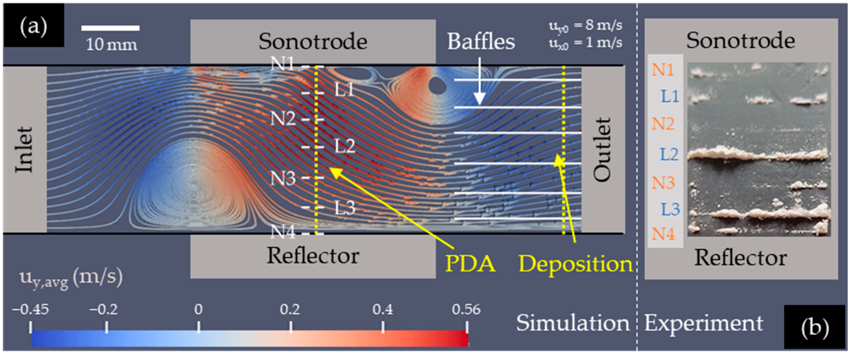
2.1. Process Scheme and General Set-Up

The principle scheme of the acoustic fractionation process to be operated in this investigation is presented in Figure 3a. The aerosol flow enters the fractionation device, surrounded by a sheath flow, from the left-hand side and passes through the acoustic field for a specific residence time. During this transit, the particles are fractionated in two distinct fractions within the acoustic field. In the applied setup, the acoustic field consists of three acoustic velocity lobes and four acoustic velocity nodes spanned between sonotrode and reflector. According to the literature, larger particles are expected to move to the acoustic velocity lobes, while smaller particles should accumulate in the acoustic velocity nodes.

Figure 3b shows the implementation of this scheme used in the deposition measurements. The particle-laden aerosol enters the device in-between baffles, leading the flow into the acoustic velocity lobe area. At the front of the device, a secondary air intake draws additional sheath gas into the flow chamber, leading into the acoustic velocity node region. The baffles in the device separate the acoustic velocity node and lobe regions throughout the device, except for the area of the acoustic field in-between sonotrode and reflector.

2.1.1. Acoustic Sources and Acoustic Field Parameter

Three different kinds of acoustic sources were employed. A low-power 50 kHz encapsulated Dantec 13L10 device (DANTEC/INVENT Measurement Technology GmbH, Ettlingen, Germany) was utilized for visualization and levitation. An ultrasound source from Hielscher (Hielscher Ultrasonics GmbH, Teltow, Germany) was used providing low-to-mid-amplitude ultra-sound at a frequency of 30 kHz. For the final experiments, Branson 184 V (Branson Sonic Power Company, Danbury, CT, USA) units were used providing mid-to-high-amplitude ultrasound at a frequency of 20 kHz. For the experiments presented here, the Branson device has been adapted because of the availability of multiple devices and accessories, including various sonotrodes with horns of different shapes and sizes, ensuring reliability, versatility, and the ability to provide a wide range of acoustic amplitudes with an elongation range of ξ_PP = 65–137 µm. The ultrasound generator’s characteristic curve is summarized in the power-to-elongation table listed in

Table 1. Characteristic power curve ultrasound generator Branson 184 V with 34 mm sonotrode.

US-Setting (%)	20	30	40	50	60	70	80	90	100
Power input (W)	80	95	108	123	145	160	176	196	207
Elong.pp (µm)	65	79	90	101	108	116	126	134	137

.

The application of 20 kHz ultrasound at the lower limit of ultrasound frequency has the advantage of a longer wavelength, increasing the overall scale of the acoustic fractionation device. For the experimental set-up (20 kHz) with three lobes and a resonance length of l_r ≈ 25.7 mm (1.5 λ), the maximum gas velocity difference is found to be up to 80 m/s in one period. The respective acoustic amplitude of u_ac ≈ 40 m/s is gained by the sonotrode elongation of ξ ≈ 67 µm due to resonance amplification from the acoustic energy input (equivalent to u_ac0 ≈ 8 m/s). The energy density range of the acoustic field generated by the experimental setup begins with E_ac ≈ 170 Ws/m³ at the upper end of the transition zone [35], where low-amplitude ultrasound transitions to high-amplitude non-linear ultrasound and extends up to E_ac ≈ 850 Ws/m³ [14]. The resonance distance l_r is set with precisely machined distance pieces. The influence of resonance misalignment was analyzed using distance pieces that are 5% larger and smaller than the resonance distance.

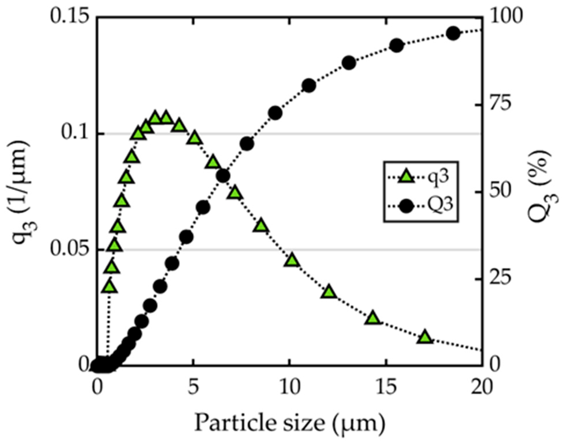
2.1.2. Particle System

The commercially available Potters Spheriglass 5000 CP00 (SPG 5000) (Potters Industries LLC, Malvern, PA, USA) particles were used in the course of the reported experiments. These silicon-oxide particles have a narrow particle size distribution, a particle-number-based median size of d_{50,0 BSM} = 2.6 µm, and a material density of ρ_matSPG5000 = 2500 kg/m³. With these particle properties, it is well positioned in the property range which the extant literature reports to result in property-dependent acoustic fractionation. Figure 4 shows the distribution frequency and the cumulative particle size distributions.

2.1.3. Particle Dispersion System

The particles are suspended in an air stream via a Palas RBG 1000 brush disperser (Palas GmbH, Karlsruhe, Germany) equipped with a C-Type head and a 7 mm piston. The piston length is 70 mm and contains m_p,p = 2.9 g for SPG5000 particles. The piston feed velocity is set to values between 10 mm/h and 150 mm/h and used with pre-pressures of p_D = 2 bar and p_D = 4 bar during the measurements, resulting in particle dispersion mass flow rates from $\stackrel{.}{{\mathrm{m}}_{\mathrm{p},\mathrm{p}}}$ ≈ 0.4–6 g/h.

2.1.4. Cross-Flow Through Experimental Setup and Aerosol Capture

The gas flow through the experimental domain is driven by a centrifugal blower mounted downstream of the device and operated in suction mode. It is equipped with a HEPA-Filter to prevent contamination of the surrounding air. The blower is operated at a volume flow rate that ensures a safe collection of the entire aerosol from the particle disperser. The aerosol inlet and blower-controlled gas outlet are tailored to produce a continuous and homogeneous flow through the experimental setup at velocities that can be varied in the range of u_chamber = 0.5–2 m/s. The outlet is equipped with a holder for glass fiber filters (Whatman GF/F and GF/D), which is utilized for local particle sampling in the deposition experiments.

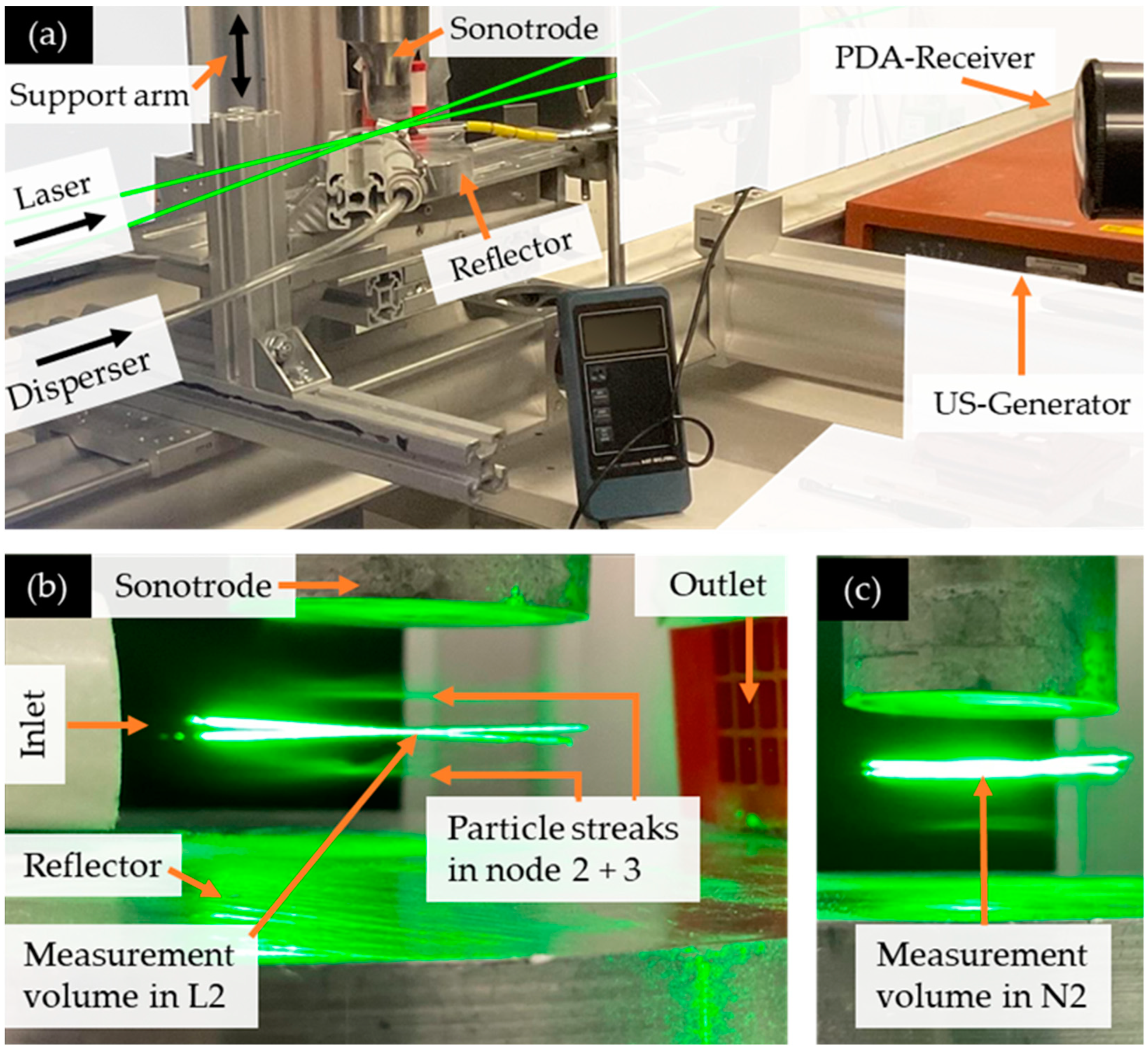
2.2. Methods and Measurement Set-Up

2.2.1. Phase Doppler Anemometry

Phase Doppler Anemometry is an extension of the Laser-Doppler-Anemometry approach. The measurement volume is spanned by the intersection of two laser beams. The two laser beams originate from a single laser source, yet are frequency-shifted by means of a Bragg cell. This results in the formation of a planar moving light intensity pattern in the intersection of the laser beams. The dynamic illumination peaks called fringes are at a fixed and calculatable distance to each other, which depends on the frequency shift between the laser beams. A particle passing through these fringes scatters the laser light due to reflection and refraction. In a detector, the scattered light of the particle is recognized. The scattered light intensity of a particle traversing through the measurement volume exhibits a peak each time a fringe is penetrated. By evaluating the time between these recognized peaks and subtraction of the fringe movement itself, the in situ particle velocity can be determined. In Phase Doppler Anemometry, multiple detectors are employed to track phase differences in the scattered light. The phase shift between the recorded signals is contingent upon the size, respective of surface curvature of the light-scattering particle [38]. This phase tracking enables the calculation of the in situ particle size. By scanning through the resonant acoustic field with this method, it is possible to directly measure local changes in particle velocity, particle number density, and, most important, particle size.

The Phase-Doppler-Anemometer (PDA) from Dantec (DANTEC DYNAMICS A/S, Skovlunde, Denmark) consists of a Burst Spectrum Analyzer BSA P600-1D, a FiberPDA-Receiver, and a 532 nm laser source with a beam splitter and Bragg cell. The system is operated with the manufacturer’s BSA-Flow software (Version 6.71.00.05), which includes the Particle Sizing Add-On. The receiver is positioned at an off-axis angle of 29° relative to the laser beam direction, aiming for the optimal location of first-order refraction. The PDAOpticalConfiguration-tool is employed for the purpose of conducting a confidence of linearity analysis. The extensive peak (89.47%) at the confidence of linearity level around the scattering angle of 29° makes it less sensitive to misalignment. The receiver surface is situated at 500 mm distance of the measurement volume. Aperture plate A is positioned in front of the receiver to match the measuring particle size range to the particle size distribution. The length of measurement volume is limited to 50 µm by setting the aperture level accordingly. Following the alignment procedure, a sensitivity analysis of the measured particle size distribution and the particle number density was conducted. The reference settings found are photomultiplier sensitivity voltage of 1100 V, gain factor of 10 dB, laser power of 316 mW, disperser pre-pressure of 3 bar, and particle feed rate of 0.4 g/h. A measurement duration of 60 s results in a counted number of particles of around 27 thousand in the reference system without ultrasonic radiation. Figure 5a shows the entire setup and Figure 5a,b detail views of the PDA-laser at the measurement positions L2 and N2. With a precision machined target and a precise X-profile adjustment system, the laser intersection (measurement volume) was set to 19 equidistant measurement positions during this investigation. The measurement locations with their respective positions in the metric and wavelength domain are summarized in

Table 2. PDA Measurement positions in the acoustic field. Blue: acoustic velocity lobe locations; Orange: acoustic velocity node locations.

Position	mm	2.2	3.2	4.3	5.4	6.4	7.5	8.6	9.7	10.7	11.8	12.9	13.9	15.0	16.1	17.2	18.2	19.3	20.4	21.4
	λ	1/8	3/16	1/4	5/16	3/8	7/16	1/2	9/16	5/8	11/16	3/4	13/16	7/8	15/16	1	17/16	9/8	19/16	5/4
Id.				L1				N2				L2				N3				L3
#		1	2	3	4	5	6	7	8	9	10	11	12	13	14	15	16	17	18	19

.

2.2.2. PDA Measurement Procedure

The execution of the measurements at each measuring point follows the predefined measuring procedure listed in

Table 3. PDA measurement procedure.

#		1	2	3	4	5	6	7	8	9	10	11	12	13	14	15
US Power	%	0	20	25	30	0	35	40	45	0	50	65	0	80	95	0
	W	0	82	90	98	0	106	114	122	0	130	154	0	178	202	0

. This measuring procedure serves to ensure that the measurements are carried out in a standardized sequence in order to maintain identical boundary conditions and comparability of the results between the measuring positions. The measurement procedure has been designed to account for two known runtime-related issues that occur in acoustic fractionation set-ups. First, during operation, particularly at elevated acoustic amplitudes, the sonotrode temperature rises due to dynamic deformation. This changes the wave propagation in the sonotrode material and results in a frequency drift. Second, the particle disperser forces the powder, driven by a piston, into the dispersion brush. The continuity of the particle mass flow can be affected by uneven filling and friction-related compression of the particle reservoir. In the measurement procedure, this is accounted for by incorporating measurement phases with disabled acoustic field. With these phases, the sonotrode has time to cool down and a drift in the reference particle concentration can be tracked. During the measurement procedure, frequency drift and the particle load are monitored. The acoustic frequency was allowed to deviate ±0.25% from the base frequency f_US = 20,000 Hz. The measurement is considered successful as long as the acoustic frequency still exceeds f_US,hot = 19,950 Hz and no significant drift in the particle feed is observed.

2.2.3. Filter Deposition Set-Up

In the deposition experiments, an acoustic fractionation device is used, as shown in the detail cut in Figure 6a. The filter device is 3D-printed by fused deposition modeling with polylactic acid filament on a Cura Ultimaker S3 (Ultimaker B.V., Geldermalsen, The Netherlands). The additive manufacturing fabrication method is advantageous for the implementation of precise complex structures, including the sealed sonotrode and reflector protrusions and the aerosol inlet. Furthermore, it is necessary for the realization of the required fine baffle structures that separate the acoustic velocity lobe and node regions before and after the acoustic field. Geometries manufactured by fused deposition modeling can have scaling issues and a significant surface roughness in stacking direction. The manufactured devices are checked for dimensional accuracy and the main surface roughness is oriented in flow direction. It is considered that the influence of geometric deviations and surface roughness on the flow behavior are negligible, given the energy input from the acoustic field. The particles are deposited in a particle trap at the device outlet. At the outlet, glass fiber filters (Whatman GF/F and GF/D) are mounted on a filter support in front of the downstream centrifugal blower. The device’s cross-section increases in front of the filter stage at the outlet to provide larger filter surface, A_Filter = 2400 mm² (A_US = 1029 mm²), and reduces pressure change during the 12 min operation of each measurement. To keep the gas velocity through the chamber constant and adapt for the increasing pressure loss of the filter media, the centrifugal blower revolution rate is increased. The particles that were deposited in front and on the filter material were sampled, weighted, and characterized in a laser diffraction spectrometer. A characteristic pre-filter deposition pattern is shown in Figure 6b. The baffles are placed in the center between the adjacent acoustic velocity node and acoustic velocity lobe. The 0.6 mm thin walls are thought to maintain the acoustically fractionated particles in the streaks into which they are forced by the acoustic field. Simultaneously, they are expected to reduce the size and intensity of secondary flow structures.

3. Results

The analytical solution for the one-dimensional gas velocity distribution of a standing acoustic wave, as discussed in Section 1.2.2, and the behavior of particles in response to the acoustic forces, as described in Section 1.2.3, are analytically derived. While numerical and analytical approaches provide insight into the assumed integral and differential changes in particle velocities and positions, empirical experimental proof or validation is missing. For comparison purposes, the Phase Doppler Anemometry investigation results at the locations of the acoustic velocity lobes and acoustic velocity nodes are of particular interest since the differences in the gas condition and properties that surround a particle are most pronounced (see Section 1.2.2). All positions in-between are reported to reassemble a gradual transition from the highly dynamic (lobe) to a stagnant flow (node) condition. For this reason, the Phase Doppler Anemometry results presented and discussed are primarily focused on the positions of sound velocity nodes and lobes. The second and third acoustic velocity node (N2, N3), as well as acoustic velocity lobes (L2, L3), present lobe and node positions in general.

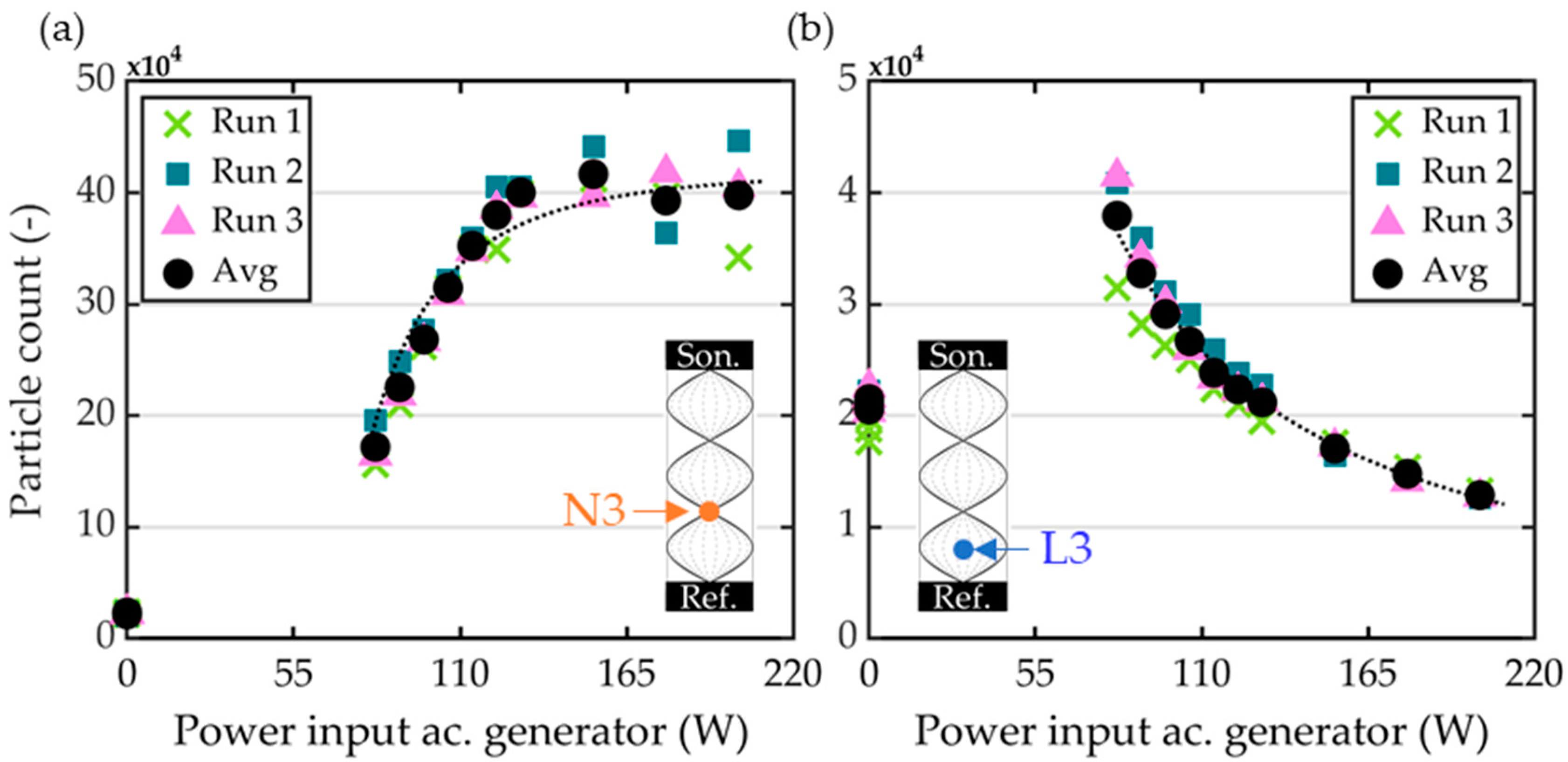
3.1. Particle Velocity Changes Due to Acoustic Radiation

With the Phase Doppler Anemometry measurement system, the in situ velocities, the number concentration, and the respective size distributions of the particles are measured at a precise location in the acoustic field. The raw data obtained by the PDA measurement system are exported into the software MATLAB (Version 9.12.0.1884302-R2022a) to create the presented figures. For Figure 7, the dataset entries are binned according to the measured particle velocity, with a binning width of 1 m/s and probability normalization. Figure 7a shows the particle velocity probability distribution at the acoustic velocity node and, in Figure 7b, at the acoustic velocity lobe. The reference case without acoustic radiation is represented by the light green blocks. In the reference case, the vast majority of the measured particles (close to 100%) have a particle velocity in the y-direction—which is the direction pointing from the sonotrode to the reflector—ranging around u_p ± 1 m/s. The slight offset in the positive direction can be attributed to differences in the sonotrode and reflector geometry and their influence on the overall flow. It is to be expected that small fluctuations in the velocity of both gas and particles occur due to the mixing and entrainment of the aerosol stream with the sheath flow (secondary intake). As the acoustic amplitude increases (Figure 7a), the width of the particle velocity distribution in the acoustic velocity node increases slightly, but still significantly. The Phase Doppler Anemometry results demonstrate a gradual smearing of the acoustic nodes with the increasing acoustic intensity; this is particularly relevant in comparison to the one-dimensional non-linear acoustic standing wave. The frequently used one-dimensional analytical gas velocity distribution is unable to account for these effects, raising concerns about the reliability of the predictions made by calculations describing particle dynamics. The observation made with the Phase Doppler Anemometry is consistent with the findings of CFD simulations, which demonstrate that acoustic velocity nodes are no longer stagnant nor discrete points of stationary gas, but rather comprise an area of low-amplitude fluctuations and acoustic streaming [14]. In the acoustic velocity lobe (Figure 7b), the width of the particle velocity distribution also increases. But, instead of reassembling a normal distribution, the histogram flattens significantly, even for low amplitudes. Along all particle velocity classes, the probability is evenly distributed. Increasing the amplitude solely changes the distribution width from P_US = 83 W (20%) between −11 and +10 m/s and a small peak in the center to P_US = 202 W (95%) with a distribution width of −22 to +21 m/s and small peaks in the center and the edges. The observed uniform particle velocity distribution in the acoustic velocity lobes is consistent with the gas velocity distribution found in simulations of intense ultrasounds.

3.2. Acoustic Influence on Local Particle Number Density

Particles dispersed in an acoustic resonant field congregate at acoustic velocity nodes and lobes, contingent on the specific characteristics of the particles in question (see Section 1.2.3). A change in the local particle concentration is a paramount indicator for substantiating this assumption. Changes in the particle number density due to acoustic radiation directly affect the number of counts recognized in the measurement volume during the Phase Doppler Anemometry measurements. To ensure that the measured particle number density variations are independent of the particle seeding process, the particle dispersion continuity is monitored. In multiple nonradiated-state measurements, the relative standard deviation of the particle count due to the seeding process is in the order of magnitude of 4%. Between different measurement campaigns, the deviation for the non-radiated state can be up to 6%. The uncertainty in the seeding density associated with the seeding process is monitored and documented. A compensation for its influence could be implemented during the data post-processing stage. With regards to the variations in the particle concentration due the acoustic field (up to ×20), these fluctuations are considered of secondary importance. Figure 8 illustrates the primary data of the particle count in relation to the acoustic intensity and location within the acoustic field.

In the acoustic velocity node (Figure 8a), the particle number density increases significantly with the acoustic field intensity, asymptotically approaching a saturation particle count of approximately 450,000 particles. In the acoustic lobe (Figure 8b), the particle number concentration increases in the lower amplitude acoustic field, followed by a decrease in the particle count with the increasing amplitude. In the acoustic velocity lobes, the slope of the particle count in the acoustic radiated cases is subject to slight influence from the seeding concentration (Figure 8b—Run 1 and Run 3), yet the underlying trend remains consistent. While an accumulation of particles is observed and confirmed in the acoustic velocity nodes, a decrease in the particle count is found for the lobes.

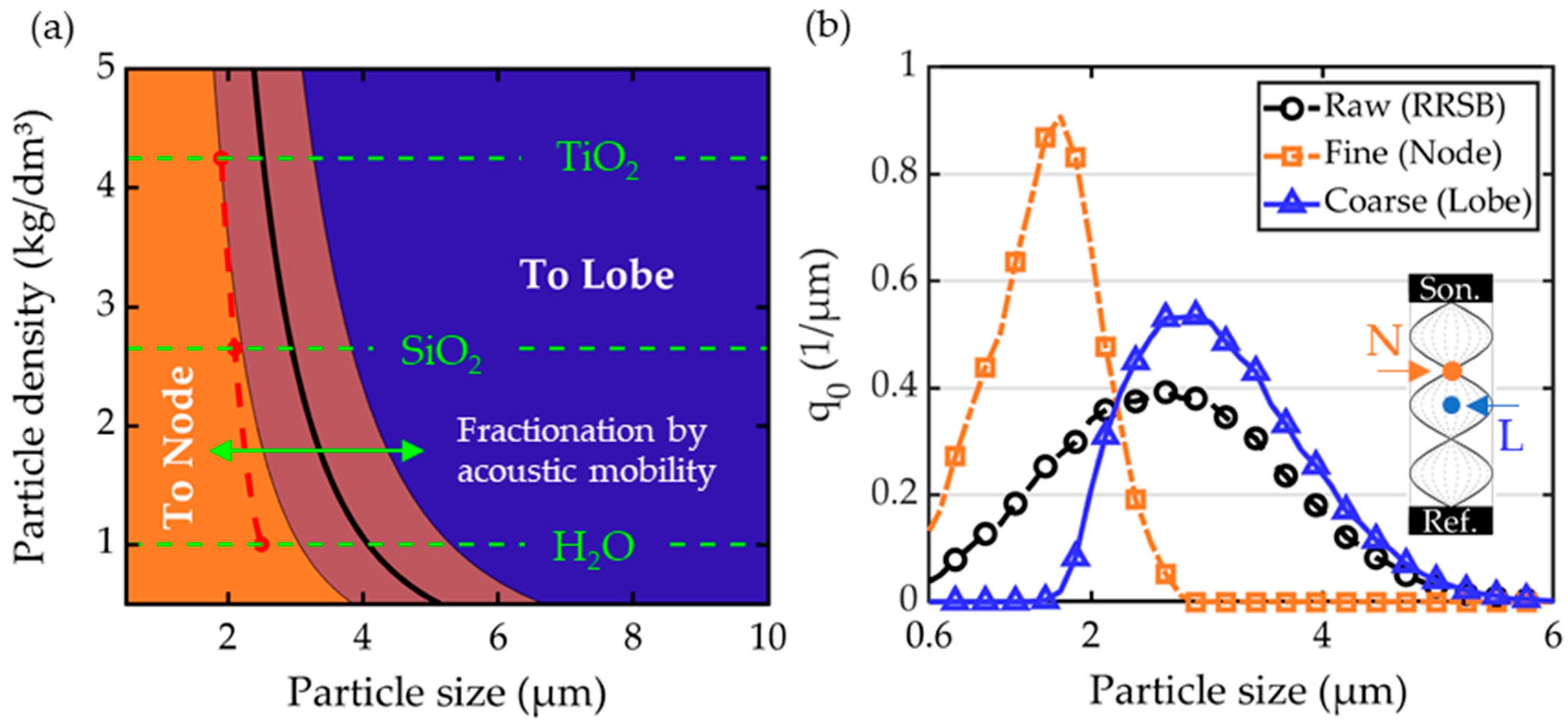
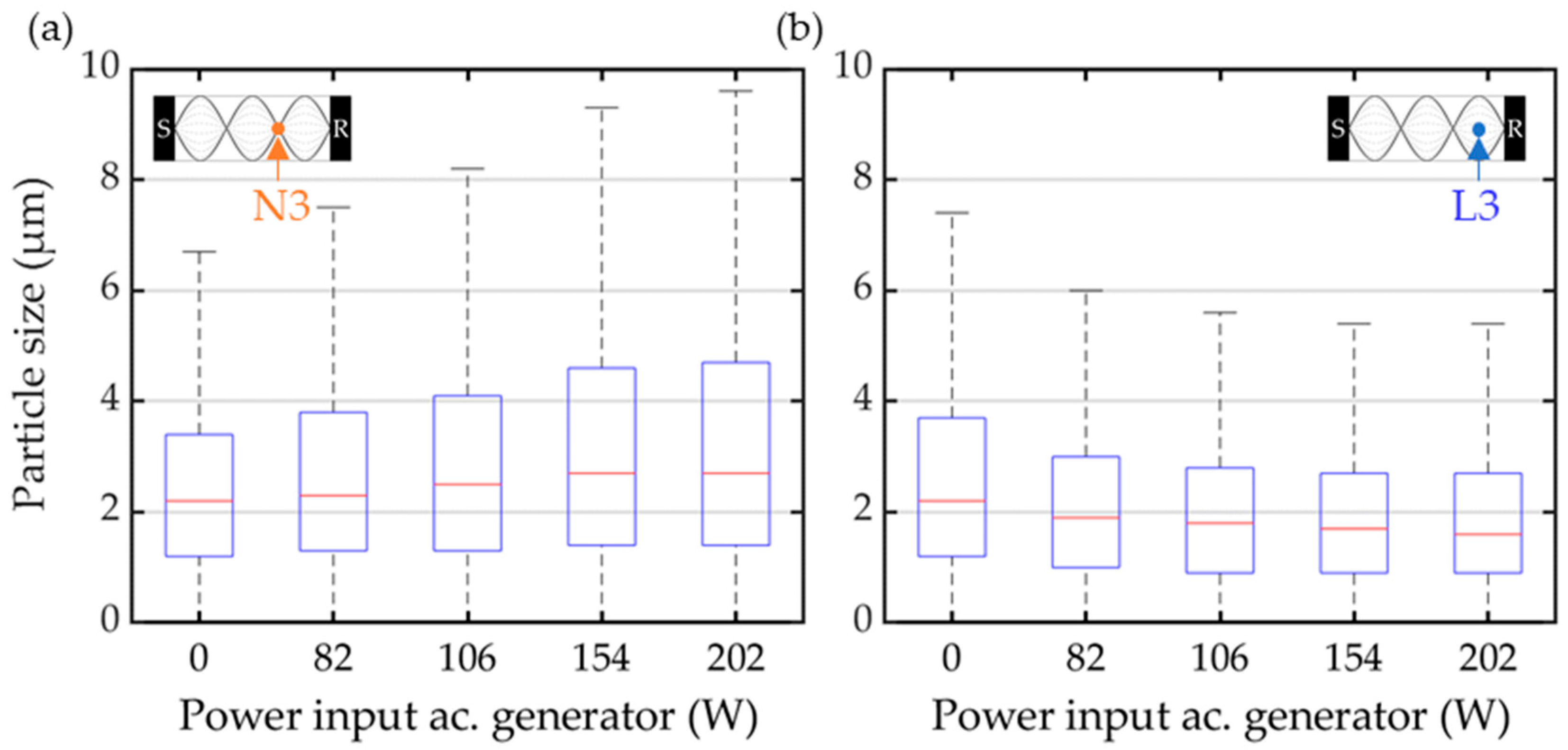
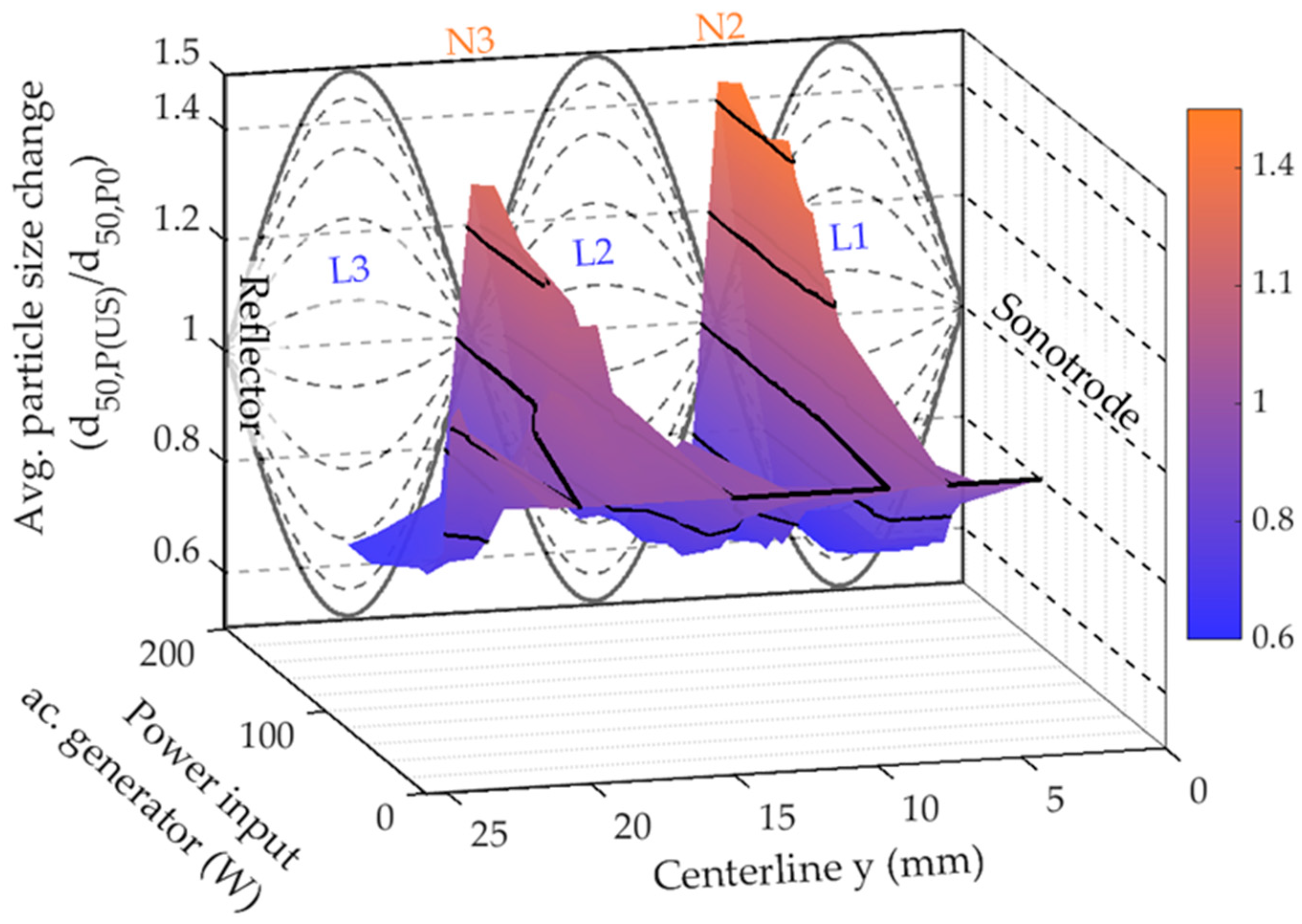
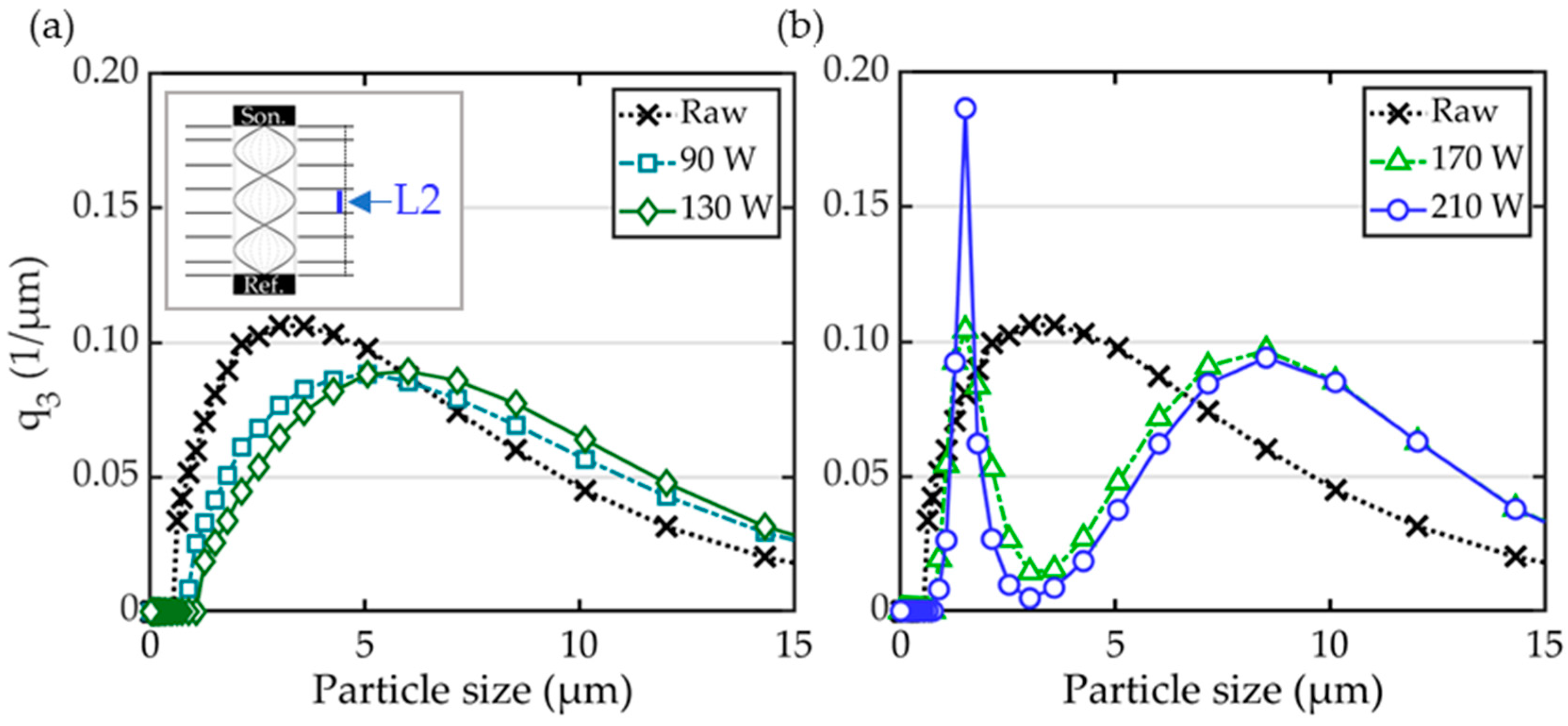
3.3. Particle Size Dependence on Acoustic Irradiation

The forces acting on particles in an acoustic field are reported to be particle-property-dependent (Section 1.2.3) and should result in selective particle fractionation. Accordingly, the in situ particle size distribution obtained by Phase Doppler Anemometry are expected to be dependent on the acoustic intensity. In Figure 9a, the averaged particle diameter measured in the acoustic velocity lobe (L3) and node (N3) is shown as the dependence of the acoustic power input. In the acoustic velocity node (N3), the mean particle diameter exhibits an increase from d_pm0 ≈ 3.2 µm to d_pmN202 ≈ 4.5 µm, whereas in the acoustic velocity lobe (L2), there is a decrease in the mean particle diameter from d_pm0 to d_pmL202 ≈ 1.9 µm. In Figure 9b, the obtained particle size distribution for an acoustic power input of P_ac = 90 W and P_ac = 202 W at the acoustic velocity lobe (L3) and node (N3) are compared with the reference case without ultrasonic radiation (black/raw). In the acoustic lobe (L3), with the increasing power input, the share of small particles increases, while the share of particles larger than 3.5 micron is significantly reduced. In the acoustic node (N3), with the increasing power input, the share of particles below three microns significantly decreases, while the share of larger particles increases. These experimental results confirm the size-selective fractionation of particles in the acoustic fractionation process. The measured alterations in the particle size distribution are inverted to those predicted by the analytical approach (Section 1.2.3). In the box-plots shown in Figure 10, the dependence of the particle size distribution from the acoustic energy input at the third acoustic node (N3) and lobe (L3) is summarized in more detail. The box-plots are derived from the experimental PDA data by using the MATLAB ’boxplot’ function. The applied whisker value of 1.5 corresponds to ±2.7 σ and a coverage of ~99.3% of the dataset. In the function, the remaining 0.7% is considered as outlier. At the acoustic velocity node (N3/Figure 10a), the particle size distribution width widens, while at the acoustic lobe (L3/Figure 10b), it is narrowing with increasing acoustic amplitude. In the acoustic velocity node (N3), the median particle diameter increases with the acoustic energy input, while it decreases at the velocity lobe (L3).

The information on the particle number density and particle size evolution favor the assumption that most particles are acoustically focused at the acoustic nodes, yet a subfraction of particles in the d_p = 2 µm size range is accumulated in the acoustic lobes. This is particularly interesting in anticipation of the acoustic deposition measurements discussed later.

In the course of the performed Phase Doppler Anemometry measurements, several different measurement locations have been investigated (see Section 2.2.2). For all nodal regions, an increase in the particle concentration and the mean particle diameter with the increasing acoustic power input has been observed. For all of the lobal area, the observed particle concentration behaved as reported in Section 3.2, while the mean particle diameter decreased with the increasing acoustic power input. In Figure 11, the change in the normalized average particle size (in reference to the unradiated state) dependent of the acoustic power input and the location in the acoustic field is sumarized.

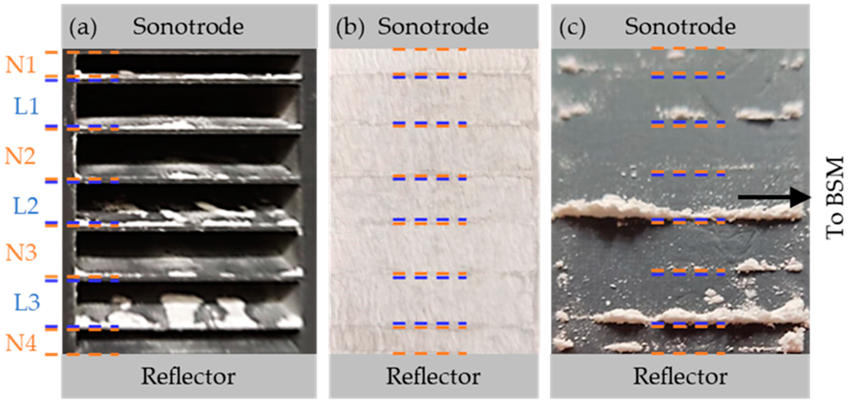
3.4. Filter Deposition Experiments

The Phase Doppler Anemometry measurements demonstrate a significant difference in the particle size distribution and particle concentration between the nodal and lobal regions for the elevated acoustic power input. To ascertain whether these fractionated particle bands persist in this grouped state after passing through the acoustic field, the particles are deposited through filtration and ex situ characterized by weighing and laser diffraction spectrometry. The exemplary result of a particle deposition experiment is shown in Figure 12. Figure 12a shows the particle depositions that settle in front of the filter media. Figure 12b shows the particle laden filter. Figure 12c illustrates the sampled deposition pattern after an acoustic deposition measurement with an acoustic energy input of P_US = 123 W (50%), a superficial gas velocity u_gas,0 = 0.81 m/s, and a particle mass flow $\stackrel{.}{{\mathrm{m}}_{\mathrm{p}}}$ = 1.04 g/h for 12 min. During the measurement period, a calculated mass of particles m_p,disp. = 0.207 g was dispersed. The mass of particles deposited on the filter was found to be m_p,filter = 0.085 g, while the mass of particles deposited in the chamber was m_p,chamber = 0.11 g. These two values collectively account for 94 m.% of the dispersed particles. The missing 6 m.% of particles are losses attributed to the dispersion and subsequent handling process. As it becomes apparent in Figure 12c, the vast majority of particles are sampled behind the second lobe (L2), the third lobe (L3), and the fourth node (N4). The uneven particle accumulation is reproducible at an elevated acoustic power input. Due to the spatial proximity of the particle samples behind L3 and N4, joint sampling was conducted. The small amount of deposited particles behind the clean nodal sampling positions (N2 + N3) was found to be insufficient to measure a meaningful particle size distribution in the laser diffraction spectroscopy device. Accordingly, the evaluation focuses primarily on the particles cleanly sampled behind the second acoustic velocity lobe (L2) which have been ex situ characterized by laser diffraction spectroscopy. The resulting particle size distributions are shown in Figure 13a for the lower acoustic power input, respectively, in Figure 13b for the high acoustic power input.

At a lower acoustic power input, the particle size distribution of the particles sampled behind the second acoustic lobe is significantly shifted to larger particle sizes in comparison to the feed material (Figure 13a). The share of smaller particles (below 6 microns) is reduced with the increasing acoustic power input. The share of larger particles (larger than 6 microns) is increased. The modal value changes from d_p,mod0 ≈ 3 µm to d_{p,mod_130} ≈ 6 µm. At a higher acoustic power input (Figure 13b) the particle size distribution changes considerably. It is bimodal, with the main modal value significantly shifted to a higher particle size of d_{p,mod2_210} ≈ 8.5 µm and a second modal spike at a particle size of d_{p,mod1_210} ≈ 1.5 µm. Particularly worth emphasizing is the almost full absence of particles of the three-micro-meter class. For a lower acoustic power input, the trend in the resulting particle size distribution of the deposition measurements (behind L2) reassembles the change observed in the acoustic velocity nodes (N) of the Phase Doppler Anemometry measurements. The reproducible behavior differs significantly. The in situ PDA results diverge from the downstream ex situ results. This difference is expected, and the implications are discussed in Section 4.

4. Discussion

In [12], it has been found that the acoustic velocity nodes (N) are unselective accumulation locations trapping all particles that enter these regions. In contrast, the acoustic velocity lobes (L) are selective accumulation locations, only able to attract larger particles as long as they enter close enough to the lobe location. In [14], the flow structure in and especially around the acoustic field has been described, emphasizing acoustic streaming and the expansion of the acoustic field far beyond the direct acoustic irradiated zone. The gradual reduction in the acoustic intensity beyond the directly radiated area results in an early particle focusing into the pre-nodal area in front of the acoustic field. This effectively prevents larger particles from reaching their semi-stable position in acoustic velocity lobes (L). Accordingly, no large particles are found in the acoustic velocity lobes by Phase Doppler Anemometry. Solely particles that leave the acoustic nodes (N) due to selective entrainment, usually smaller particles (drag > acoustic forces), can be found in the acoustic velocity lobes (L) [14], decreasing the particle size distribution measured at the lobe significantly. These particles are forced out of the acoustic velocity nodes and driven through the acoustic field by the secondary flow structure induced by acoustic streaming. This phenomenon is frequently reported for nonlinear ultrasounds, but often neglected in the acoustic fractionation literature. In conclusion, in the acoustic velocity lobes, the particle number density decreases and the particle size distribution is shifted to smaller particle sizes. In the acoustic velocity nodes, the pre-nodal focusing of particles increases the particle number density significantly. The local mean particle size is increased and the respective particle size distribution is widened. This is in exact accordance with the findings yielded by the conducted Phase Doppler Anemometry measurements. Moreover, a notable difference in the particle size distributions between the node and lobe regions has been substantiated, providing compelling evidence for the emergence of acoustic fractionation.

In the particle deposition measurements, multiple noteworthy observations were made. First, for a low acoustic power input, the entire particle size distribution behind the acoustic lobe (L2) shifts to larger particle sizes. Second, this behavior reassembles the observation made with Phase Doppler Anemometry in the nodal (N) region. Third, for high acoustic power input, the particle size distribution found behind the second acoustic velocity lobe changes considerably; it becomes bimodal. The two modes have a particle size of d_{p,mod1_210} ≈ 1.5 µm and d_{p,mod2_210} ≈ 8.5 µm and a total absence of particles in the St ≈ 1 size range. The initial two observations can be elucidated through the adaptation and examination of the numerical simulations presented in [14]. The flow field presented in Figure 14a is derived by simulations performed using the compressible sprayFOAM solver in the CFD tool OpenFOAM. Further information on the methodology, boundary conditions, and parameters can be found in [14]. In Figure 14a, streamlines of the time-averaged gas velocity distribution are shown along the central slice through the acoustic fractionation device.

The colormap highlights the gas velocity differences in the y direction (sonotrode–reflector). Without or with the lowest amplitude acoustic radiation, the gas flow would pass through the device without any observable disturbance, but because of the non-linear effects occurring in intense ultrasounds, a secondary flow pattern is induced. It is driven by acoustic streaming from the sonotrode in the direction of the reflector and deforms the streamlines to an inverted s-shape. This flow structure generates a supplementing drag force that displaces the suspended particles. While in the Phase Doppler Anemometry measurements the vast majority of particles are concentrated in the acoustic nodes (e.g., N2), they are displaced downstream by a half wavelength. In the deposition measurement, this vast majority of particles is observed in the adjacent acoustic lobe (L2). This substantiates two findings. Firstly, the particle fractionation observed by Phase Doppler Anemometry has been verified by the deposition measurement conducted at a lower acoustic power input. Secondly, it has been experimentally demonstrated that acoustic streaming has a significant impact on the flow field within an acoustic fractionation device and the acoustic fractionation process (compare Figure 14a,b).

The analytical approach by Danilov [24] predicts an accumulation of larger particles in the acoustic velocity lobes, resulting in a local increase in the average particle size. At the acoustic velocity node, a decrease in the average particle size is predicted since smaller particles than the critical particle size accumulate in this region. The critical particle diameter is derived to d_{p_crit,Danilov} = 3.03 µm for the investigated acoustic field and particle properties. The critical particle diameter is the particle size that has the lowest directional sensitivity to acoustic forces. However, this ideal model does not consider the effects of acoustic streaming appearing and the crossflow that is used during the experiments to transport the particles through the acoustic field. In the PDA and the deposition measurements, the applied acoustic field results in an inverted behavior to that predicted in analytical models. In an acoustic velocity node, the average particle size increases, while it decreases in the acoustic velocity lobes. This discrepancy is attributed to different acoustic fractionation mechanisms. In the experiments, acoustic fractionation due to selective entrainment is observed rather than the conventional acoustic fractionation. All particles are focused on the acoustic velocity nodes far in front of the acoustic field. From there, the particles with the lowest sensitivity to acoustic forces are selectively entrained through the acoustic field by the secondary flow structure. The critical particle diameter [24] derived for conventional acoustic fractionation is still a decisive parameter for this behavior. For those particles, the drag forces are dominant and these particles are entrained from the acoustic nodes through the acoustic lobes when a significant acoustic intensity is applied. With an increasing acoustic intensity being applied, the particle size range for which drag forces due to the secondary flow structure dominate the acoustic forces becomes wider. This explains the bimodal particle size distribution and the absence of particles in the particle size range d_p ≈ 3 µm found in the deposition experiments at a high acoustic power input (Figure 13b). Larger and smaller particles experience higher acoustic forces in reference to the experienced drag force of the gas flow [14]. The particles in the critical size range are selectively entrained through the acoustic field by the acoustic-streaming-induced flow. Larger and smaller particles remain acoustically locked into the acoustic node locations in the center of the acoustic field; downstream, these remaining particle bands are shifted by a half wavelength, as observed in the deposition measurements. The particle drift is assumed to be, to a certain degree, dependent on the baffle placement. A baffle placement further upstream may interfere with the standing wave formation, but might improve the particle drift by hindering the vortex formation. With a device having the baffles placed 5 mm into the acoustic field from the downstream direction, no significant differences in the deposition pattern and results were found. Future work is needed to determine the dependence of the secondary flow structure and the particle drift from the baffle location.

5. Summary and Conclusions

Analytical and simulative investigations suggest that a selective acoustic particle fractionation process can be realized in the gas phase. An evaluation of the viability of gas-born acoustic fractionation for real-world applications is missing. Experimental studies employing Phase Doppler Anemometry and particle deposition experiments on particles suspended in an acoustic field are conducted. The findings confirm the property-dependent fractionation of particles into acoustic velocity lobes and nodes. In the Phase Doppler Anemometry measurements, the median particle diameter in the acoustic velocity lobes is found to decrease with an increasing acoustic energy input. In the acoustic velocity nodes, the particle diameter increases with the acoustic power input. This finding contradicts the conclusions reached in previous analytical studies as different acoustic fractionation mechanisms come into play. The effect observed in the experiments corresponds to acoustic-induced selective entrainment in the critical particle diameter size range. The deposition experiments demonstrate that particle streaks, that are initially acoustically focused in the acoustic velocity nodes at the center of the acoustic field, are diverted by half a wave length to the acoustic lobes when reaching the sampling area behind the acoustic field. This behavior is attributed to acoustic streaming, a secondary flow pattern that occurs in intense acoustic fields. For a low acoustic power input, the measured particle size increases with the increasing acoustic power input. For a higher acoustic power input, the measured particle size distribution becomes bimodal. These observations align and explain the behavior expected and predicted in the literature, confirming the significant impact of acoustic streaming on the fractionation process.

In conclusion, the employed acoustic field has a fractionating influence on the particles suspended in a gaseous phase. However, the appearance of secondary flow structures perturbs particle fractionation. The results obtained offer a counterbalance and reference point to the existing analytical literature. The implementation of an acoustic fractionation process, comparable to the microfluidic devices established in suspension fractionation, will be challenging for gas-born particles. The occurring secondary flow effects entrain and remix the particle fractions, impeding the fractionation process. However, for a high acoustic power input, the selective entrainment of the St ≈ 1 fraction has been confirmed in the deposition measurements. Exploiting acoustic streaming for a fractionation process that selectively entrains fractions of particles in the acoustic field seems to offer a smart and powerful alternative fractionation process for particles and conditions for that few other possibilities exist. It might be useful to implement and utilize the process of selective entrainment from the outset. For this the inlet of the particle-laden aerosol should only take place in the sonotrode-near acoustic velocity node. Secondly, the correct positions of the downstream baffles must be identified. The objective is to direct the selectively entrained particles across multiple nodes to prevent back mixing through entrainment of the flow field occurring at the end of the acoustic field.

References

1. Buchwald, T.; Ditscherlein, R.; Peuker, U.A. Beschreibung von Trennoperationen mit mehrdimensionalen Partikeleigenschaftsverteilungen. Chem. Ing. Tech. 2022, 95, 199–209. [Google Scholar] [CrossRef]
2. Bell, T.A. Challenges in the scale-up of particulate processes—An industrial perspective. Powder Technol. 2005, 150, 60–71. [Google Scholar] [CrossRef]
3. Damm, C.; Long, D.; Walter, J.; Peukert, W. Size and Shape Selective Classification of Nanoparticles. Powders 2024, 3, 255–279. [Google Scholar] [CrossRef]
4. Löffler, F. Staubabscheiden; Georg Thieme Verlag: Stuttgart, Germany; New York, NY, USA, 1988. [Google Scholar]
5. Spötter, C.; Legenhausen, K.; Weber, A.P. Separation Characteristics of a Deflector Wheel Classifier in Stationary Conditions and at High Loadings: New Insights by Flow Visualization. KONA Powder Part. J. 2018, 35, 172–185. [Google Scholar] [CrossRef]
6. Weers, M.; Hansen, L.; Schulz, D.; Benker, B.; Wollmann, A.; Kykal, C.; Kruggel-Emden, H.; Weber, A.P. Development of a Model for the Separation Characteristics of a Deflector Wheel Classifier Including Particle Collision and Rebound Behavior. Minerals 2022, 12, 480. [Google Scholar] [CrossRef]
7. Stieß, M. Mechanische Verfahrenstechnik—Partikeltechnologie 1; Springer: Berlin/Heidelberg, Germany, 2009. [Google Scholar] [CrossRef]
8. Kuger, L.; Franzreb, M. Design of a Magnetic Field-Controlled Chromatography Process for Efficient and Selective Fractionation of Rare Earth Phosphors from End-of-Life Fluorescent Lamps. ACS Sustain. Chem. Eng. 2024, 12, 2988–2999. [Google Scholar] [CrossRef]
9. Arlt, C.-R. Mehrdimensionale Fraktionierung von Feinstpartikeln Mittels Magnetischer, Kontinuierlicher Gegenstromchromatographie. Ph.D. Thesis, Karlsruher Institut für Technologie (KIT), Karlsruhe, Germany, 2022. [Google Scholar]
10. Winkler, M.; Rhein, F.; Nirschl, H.; Gleiss, M. Real-Time Modeling of Volume and Form Dependent Nanoparticle Fractionation in Tubular Centrifuges. Nanomaterials 2022, 12, 3161. [Google Scholar] [CrossRef]
11. Eckelt, J.; Maskos, M.; Wolf, B.A. Fractionation. In Polymer Science: A Comprehensive Reference; Elsevier: Amsterdam, The Netherlands, 2012; pp. 65–91. [Google Scholar] [CrossRef]
12. Sandmann, K.; Fritsching, U. Selektive Partikelklassierung in ultraschallangeregten Aerosolen. Chem. Ing. Tech. 2020, 92, 635–642. [Google Scholar] [CrossRef]
13. Sachs, S.; Baloochi, M.; Cierpka, C.; Konig, J. On the acoustically induced fluid flow in particle separation systems employing standing surface acoustic waves—Part I. Lab. Chip 2022, 22, 2011–2027. [Google Scholar] [CrossRef] [PubMed]
14. Sandmann, K.; Fritsching, U. Acoustic separation and fractionation of property-distributed particles from the gas phase. Adv. Powder Technol. 2023, 34, 104270. [Google Scholar] [CrossRef]
15. González, I.a.; Hoffmann, T.L.; Gallego, J.A. Precise measurements of particle entrainment in a standing-wave acoustic field between 20 and 3500 Hz. J. Aerosol Sci. 2000, 31, 1461–1468. [Google Scholar] [CrossRef]
16. Fan, F.; Xu, X.; Zhang, S.; Su, M. Modeling of particle interaction dynamics in standing wave acoustic field. Aerosol Sci. Technol. 2019, 53, 1204–1216. [Google Scholar] [CrossRef]
17. Arai, T.; Sato, T.; Matsubara, T. Effective Cell Transfection in An Ultrasonically Levitated Droplet for Sustainable Technology. Adv. Sci. 2022, 9, e2203576. [Google Scholar] [CrossRef]
18. Lieber, C.; Autenrieth, S.; Schönewolf, K.-Y.; Lebanoff, A.; Koch, R.; Smith, S.; Schlinger, P.; Bauer, H.-J. Application of acoustic levitation for studying convective heat and mass transfer during droplet evaporation. Int. J. Multiph. Flow. 2024, 170, 104648. [Google Scholar] [CrossRef]
19. Ran, W.; Saylor, J.R. The directional sensitivity of the acoustic radiation force to particle diameter. J. Acoust. Soc. Am. 2015, 137, 3288–3298. [Google Scholar] [CrossRef] [PubMed]
20. Fritsching, U.; Bauckhage, K. The interaction of drops and particles with ultrasonic standing wave fields. Comput. Acoust. Its Environ. Appl. Ii 1997, 25, 151–160. [Google Scholar] [CrossRef]
21. Wu, M.; Ozcelik, A.; Rufo, J.; Wang, Z.; Fang, R.; Jun Huang, T. Acoustofluidic separation of cells and particles. Microsyst. Nanoeng. 2019, 5, 32. [Google Scholar] [CrossRef]
22. Luo, X.; Cao, J.; Gong, H.; Yan, H.; He, L. Phase separation technology based on ultrasonic standing waves: A review. Ultrason. Sonochem 2018, 48, 287–298. [Google Scholar] [CrossRef]
23. Doinikov, A.A. Acoustic radiation force on a spherical particle in a viscous heat-conducting fluid. III. Force on a liquid drop. J. Acoust. Soc. Am. 1997, 101, 731–740. [Google Scholar] [CrossRef]
24. Danilov, S.D.; Mironov, M.A. Mean force on a small sphere in a sound field in a viscous fluid. J. Acoust. Soc. Am. 2000, 107, 143–153. [Google Scholar] [CrossRef] [PubMed]
25. Zhang, Y.; Chen, X. Particle separation in microfluidics using different modal ultrasonic standing waves. Ultrason. Sonochem. 2021, 75, 105603. [Google Scholar] [CrossRef] [PubMed]
26. Holwill, I.L.J. The use of ultrasonic standing waves to enhance optical particle sizing equipment. Ultrasonics 2000, 38, 650–653. [Google Scholar] [CrossRef]
27. Sajeesh, P.; Sen, A.K. Particle separation and sorting in microfluidic devices: A review. Microfluid. Nanofluid. 2013, 17, 1–52. [Google Scholar] [CrossRef]
28. Townsend, R.J.; Hill, M.; Harris, N.R.; White, N.M. Modelling of particle paths passing through an ultrasonic standing wave. Ultrasonics 2004, 42, 319–324. [Google Scholar] [CrossRef] [PubMed]
29. Imani, R.J.; Robert, E. Estimation of acoustic forces on submicron aerosol particles in a standing wave field. Aerosol Sci. Technol. 2017, 52, 57–68. [Google Scholar] [CrossRef]
30. Manneberg, O. Multidimensional Ultrasonic Standing Wave Manipulation in Microfluidic Chips. Ph.D. Thesis, Royal Institute of Technology, Stockholm, Sweden, 2009. [Google Scholar]
31. Settnes, M.; Bruus, H. Forces acting on a small particle in an acoustical field in a viscous fluid. Phys. Rev. E Stat. Nonlin Soft Matter Phys. 2012, 85, 016327. [Google Scholar] [CrossRef]
32. Karlsen, J.T.; Bruus, H. Forces acting on a small particle in an acoustical field in a thermoviscous fluid. Phys. Rev. E Stat. Nonlin Soft Matter Phys. 2015, 92, 043010. [Google Scholar] [CrossRef]
33. Online Representation of AcouSort AB. Available online: https://acousort.com/ (accessed on 7 March 2024).
34. Funcke, G.; Frohn, A. 29 O 02 Numerical investigation of the influence of different forces on the motion of aerosol particles in a standing sonic field. J. Aerosol Sci. 1993, 24, S339–S340. [Google Scholar] [CrossRef]
35. Lerch, R.; Sessler, G.; Wolf, D. Technische Akustik; Springer: Berlin/Heidelberg, Germany, 2009. [Google Scholar] [CrossRef]
36. Weller, H.G.; Tabor, G.; Jasak, H.; Fureby, C. A tensorial approach to computational continuum mechanics using object-oriented techniques. Comput. Phys. 1998, 12, 620–631. [Google Scholar] [CrossRef]
37. Greenshields, C. OpenFOAM v10 User Guide; The OpenFOAM Foundation: London, UK, 2022. [Google Scholar]
38. Ofner, B. Phase Doppler Anemometry (PDA). In Optical Measurements; Franz Mayinger, O.F., Ed.; Springer: Berlin/Heidelberg, Germany, 2001; pp. 139–152. [Google Scholar] [CrossRef]
Figure 1. (a) Normalized gas velocity distribution obtained by the 1-D acoustic standing wave formulation. Acoustic velocity lobes (blue) and nodes (orange) are highlighted. Light green indicates the velocity distribution at t0. The color-graded lines (green to black) show the subsequent gas velocity distributions of the acoustic period with a temporal spacing of 5 µs. (b) the same as (a), but considering the non-linear behavior of the acoustic field at elevated acoustic energy level (emerging “saw tooth shape”). Blue markings at acoustic velocity lobe locations (L1–L3), orange markings at acoustic velocity node locations (N1–N4).
Powders 04 00005 g001
Figure 2. (a) The fractionation partition map of gas-born particles in resonant ultrasound, red dashed line: Data from [12] (differential approach), black line: adapted integral analytical approach from [24]. Particles on the left-hand side (orange) are acoustically forced into the acoustic velocity nodes (N). Larger or denser particles (upper right side—blue) are forced into sound velocity lobes (L). Particles in-between slowly approach target location, black line: critical particle diameter, no preferred direction. (b) Numerical calculated particle fractionation in an acoustic field adapted from [12]. Particle size distributions of the feed material (black) in the acoustic node (N) (orange) and in the acoustic lobe (L) (blue).
Powders 04 00005 g002
Figure 3. (a) Process scheme of the acoustic fractionation device, aerosol inlet between baffles leading to acoustic velocity lobes. Sheath gas flow entering from left, flowing through baffles into acoustic velocity nodes. Fractionation by inertia expected; small/light particles forced into acoustic velocity nodes, large/dense particles into acoustic velocity lobes; (b) Top-open cut of the CAD-design of the fractionation device’s physical implementation. Blue markings at acoustic velocity lobe locations, orange markings at acoustic velocity node locations.
Powders 04 00005 g003
Figure 4. Particle size distributions of the SPG5000 particles used during the investigation of acoustic particle fractionation. Obtained by laser diffraction spectrometry.
Powders 04 00005 g004
Figure 5. Experimental set-up; (a) General view of the experimental set-up showing the laser-receiver alignment and the traversing system; (b) Detail view: measurement volume in L2, scattered laser light of the PDA illuminates particle streaks occurring in acoustic velocity N2 and N3. (c) Same as in (b), but measurement volume in N2.
Powders 04 00005 g005
Figure 6. (a) A 3/4 cut of the deposition device (CAD-Design) highlighting internal design features like aerosol inlet, baffle placement, and change in cross-section between process and deposition area. (b) Image of the device’s sealing surface at the filter position (outlet); visible particle deposition in front of the filter in the lobe locations.
Powders 04 00005 g006
Figure 7. (a) Probability histogram showing the particle velocity distribution in y-direction at the third acoustic node (N3) obtained by Phase Doppler Anemometry. Green histogram for disabled acoustic source. All particle velocities in-between ±1 m/s. For increasing acoustic power input, smearing of the nodal particle velocities reassembling a normal distribution. (b) is the same as (a) for the third acoustic lobe (L3). Even low acoustic amplitudes cause a uniform and equally distributed particle velocity distribution. With increasing amplitude, the distribution width increases.
Powders 04 00005 g007
Figure 8. Change in particle count when dependent to the intensity of the resonant acoustic field. Multiple experimental runs are presented to set fluctuations in the particle dispersion process into perspective. (a) Third acoustic velocity node (N3): the particle number density increases (×20) with increasing acoustic energy input. (b) Third acoustic velocity lobe (L3): for low-acoustic-energy input, the particle number density increases to the reference situation. With increasing energy input, the particle number density decreases.
Powders 04 00005 g008
Figure 9. (a) Evolution of the average particle diameter in the third acoustic velocity lobe (L3) and node (N3) dependent of the acoustic power input. In N3 (orange), the average particle size increases with increasing acoustic power input. In L3 (blue), the average particle size decreases with increasing acoustic power input. (b) Particle size distribution (PSD) of the particles observed by PDA in N3 and L3. In N3, the PSD widens, the modal particle size increases with increasing power input. In L3, the modal particle size decreases and the PSD narrows with increasing acoustic power input.
Powders 04 00005 g009
Figure 10. Boxplot of the particle size number distribution dependent of the acoustic power input. The red lines indicate the median value, the box edges are the 25th and 75th percentile, and the whiskers are at 2.7σ. (a) At the third acoustic velocity node (N3), the median particle size increases with acoustic power input. The PSD widens. (b) At the acoustic velocity lobe (L3), the median particle size and the particle size distribution width decreases with increasing acoustic power input.
Powders 04 00005 g010
Figure 11. Colored 3D-Surface of the measured normalized average particle sizes dependent of their location and the intensity of the acoustic field. Projection of the 1D analytical gas velocity distribution at the yz-plane (background) for orientation purposes. The color map shows orange for an average particle size that is significantly larger (up to +50%) than without acoustic radiation. This is the case at the acoustic nodes N2 and N3 for elevated acoustic power input. The color map is blue for an average particle size significantly smaller (−40%) than that of the unradiated case. This is valid at the acoustic lobe locations at elevated acoustic power input.
Powders 04 00005 g011
Figure 12. Probe handling and sampling in the particle deposition measurements. (a) Particle deposits in the particle trap in front of the filter element after acoustic deposition run. (b) Particle deposits on the filter material. (c) Collected particles of the deposition measurement at the sampling table. One sample is taken from the fraction deposited behind L2, and another sample is taken from the particles in L3 and N4 combined since the immediate proximity would make separate sampling operations difficult and error-prone. The particles are ex situ characterized by laser diffraction spectrometry.
Powders 04 00005 g012
Figure 13. Particle size distribution q3 of the deposited particles behind L2. The reference case without acoustic radiation is colored black. (a) For low-acoustic-power input, the modal values and the overall PSD is shifted to larger particle sizes. (b) For higher acoustic power input the PSD becomes bimodal with modes at 1.5 µm and 8.5 µm and the absence of particles in the size range around 3 µm.
Powders 04 00005 g013
Figure 14. Comparison of the gas flow behavior in an acoustic fractionation device obtained by computational fluid dynamics (a) and the observed deposition pattern (b). The position off-set observed between the PDA and deposition experiments is caused by lateral transport with the inverted s-shape of an intense acoustic flow field. (a) Derived by CFD simulations using the methodology and boundary conditions as presented in [14]. (b) Particle deposition pattern from deposition experiments presented in Section 3.4.
Powders 04 00005 g014