

Variability of the Diurnal Cycle of Precipitation in South America


Abstract
1. Introduction
2. Materials and Methods
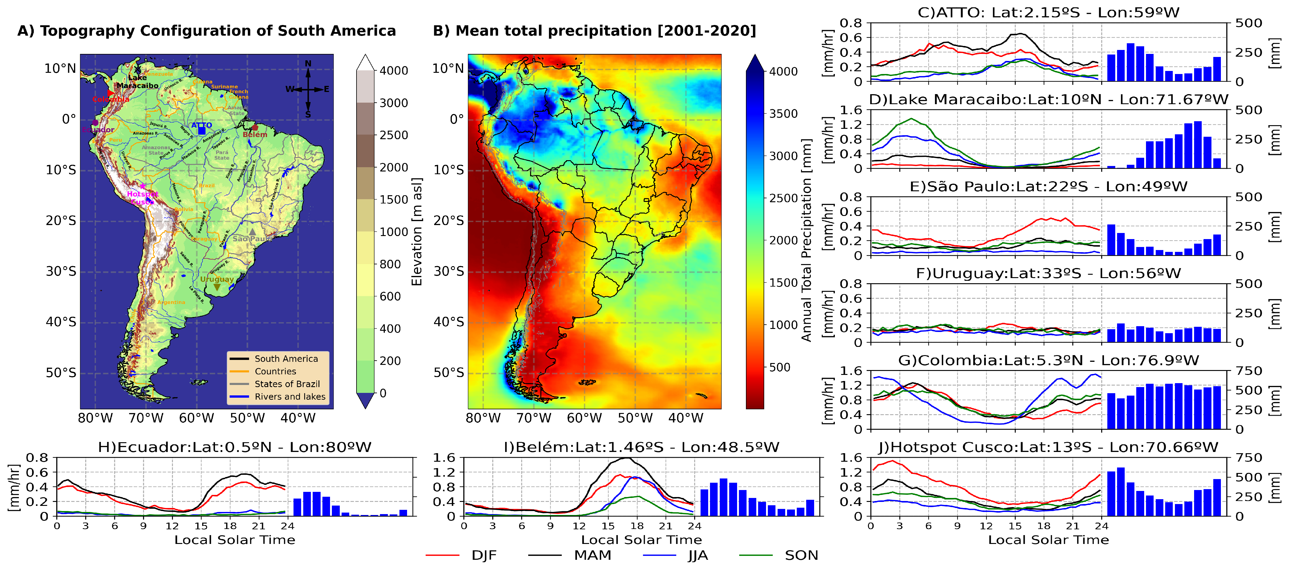
2.1. Study Area
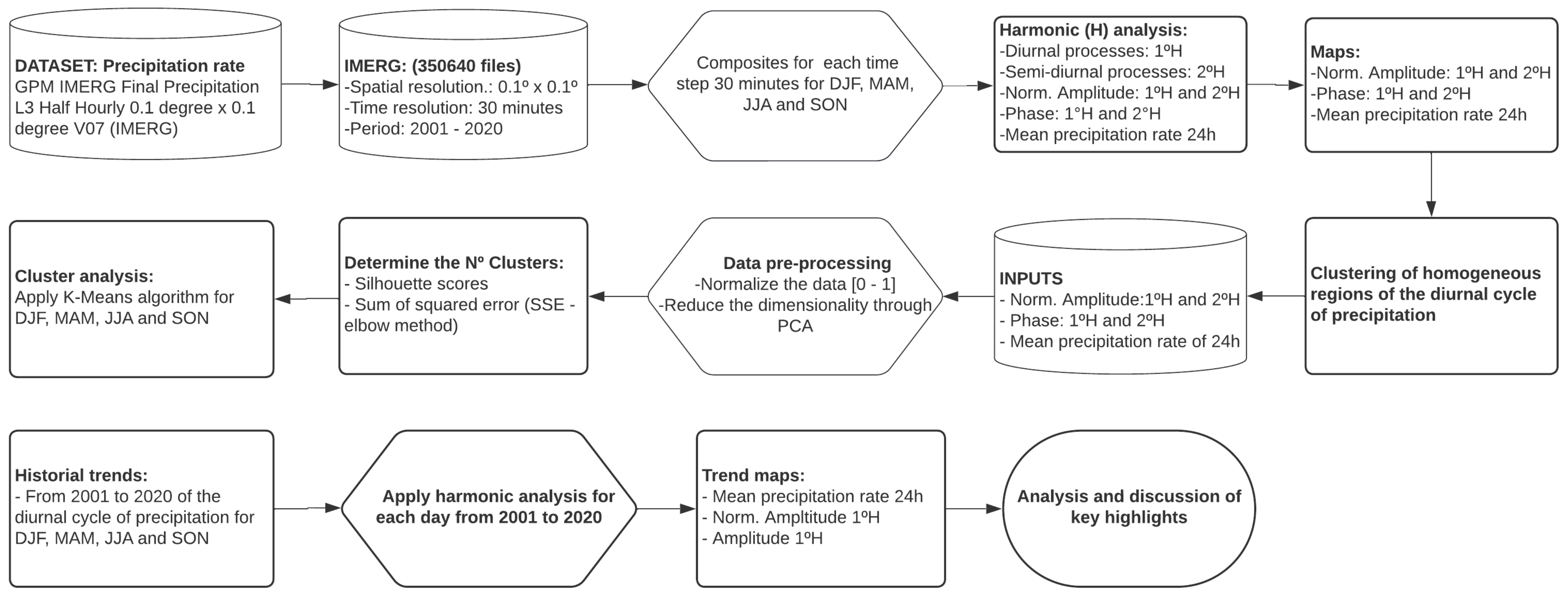
2.2. Data
2.3. Climatology of the Diurnal Cycle of Precipitation
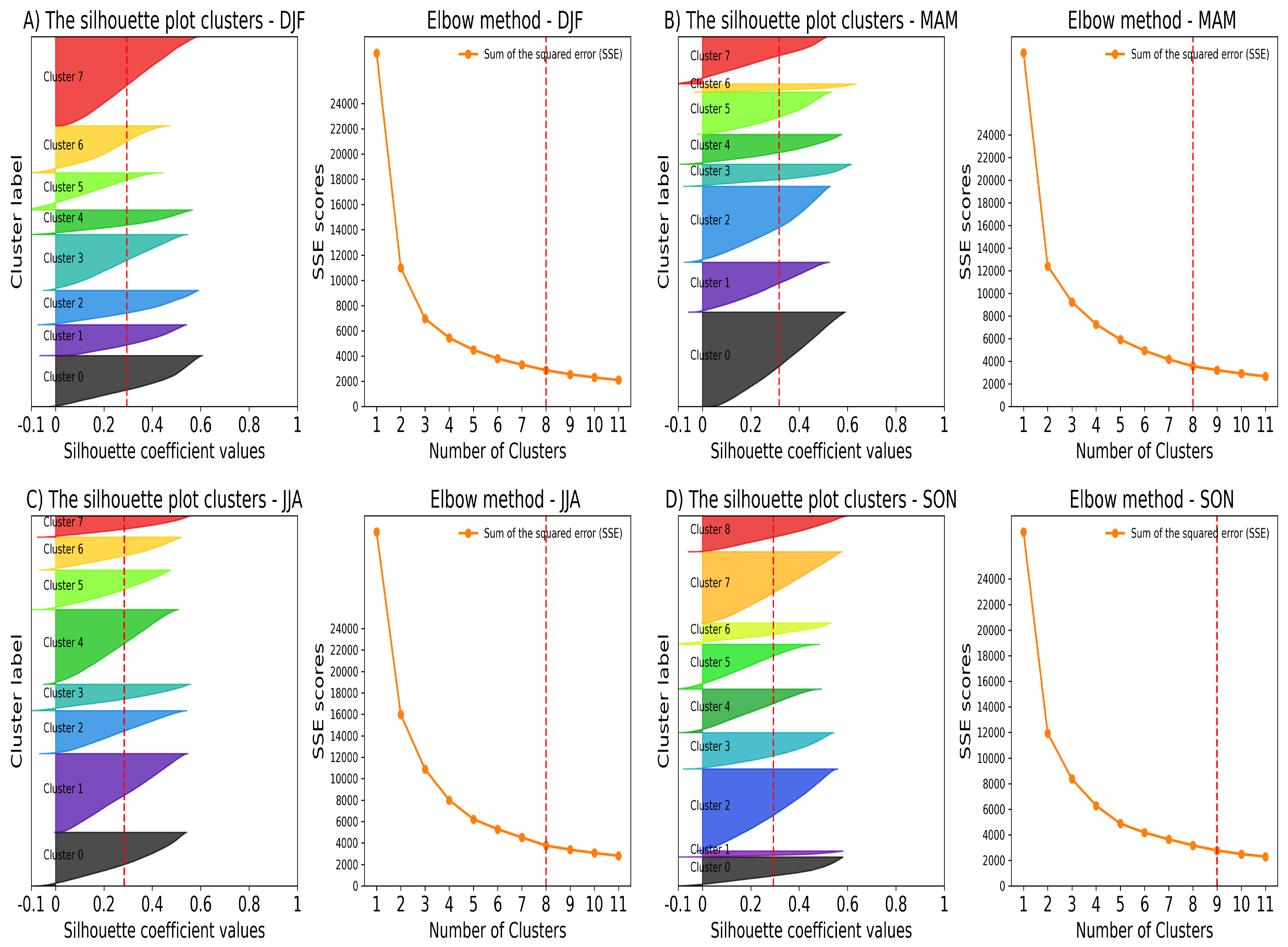
2.4. Identification of Homogeneous Regions
2.5. Trends in the Diurnal Cycle of Precipitation
3. Results
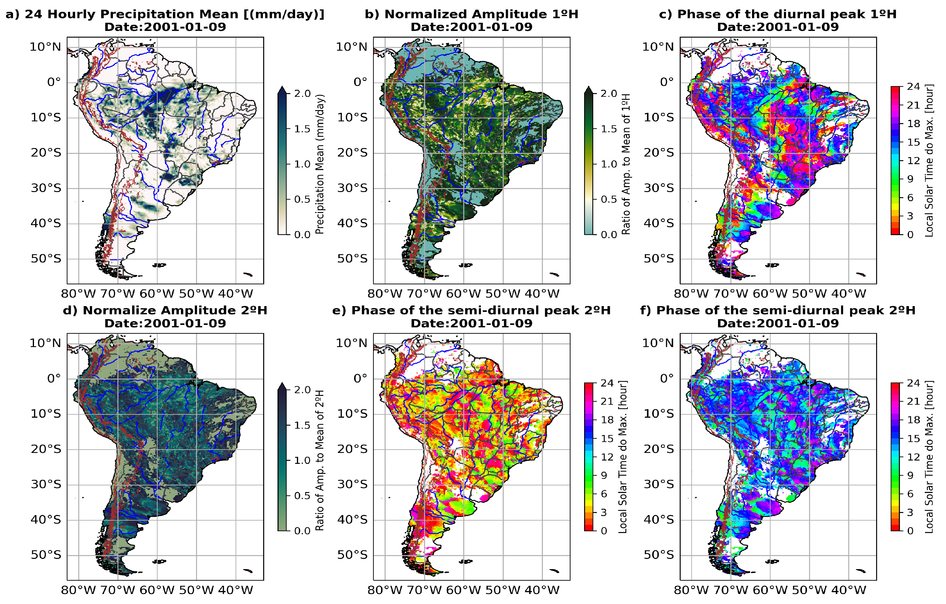
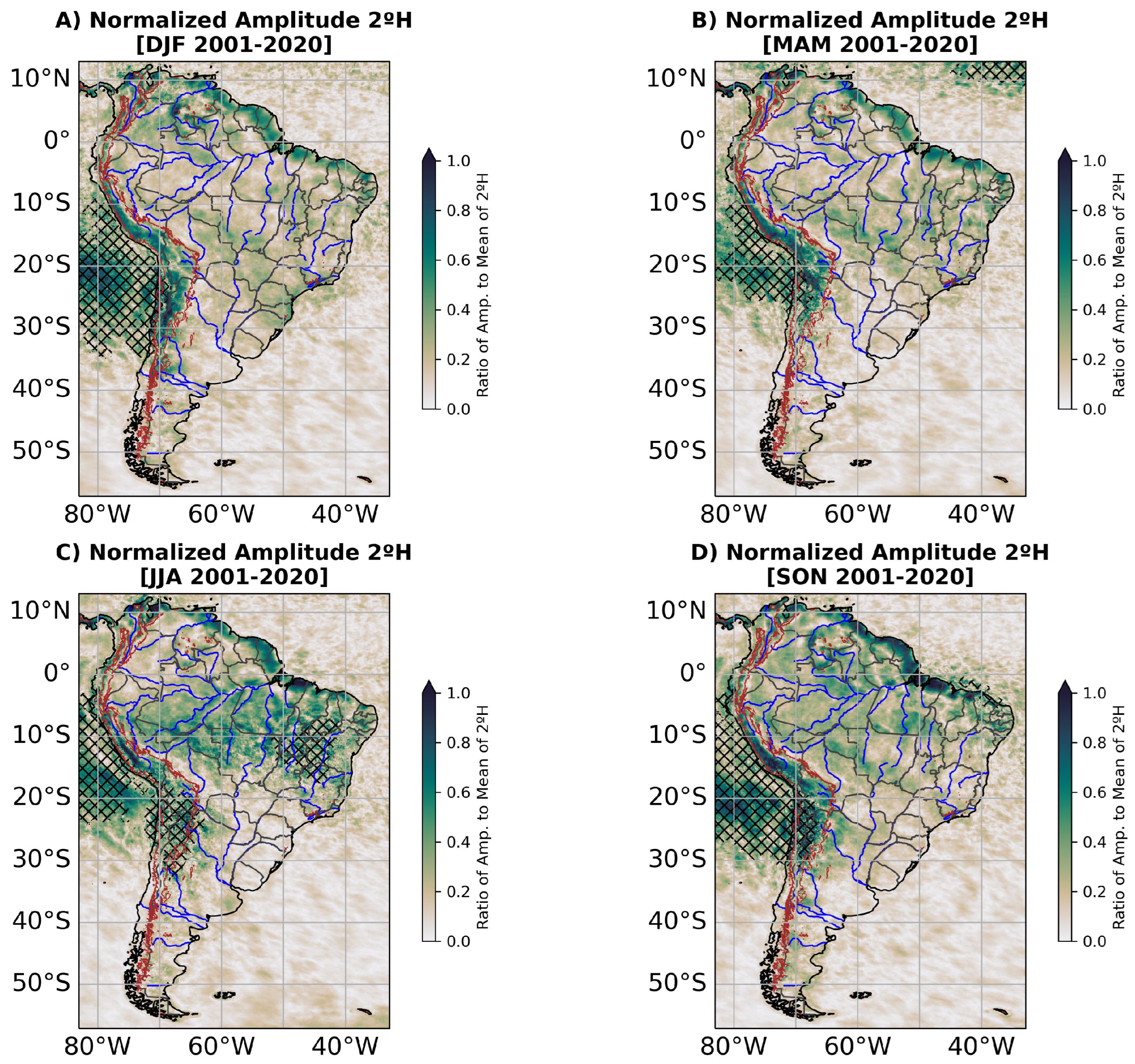
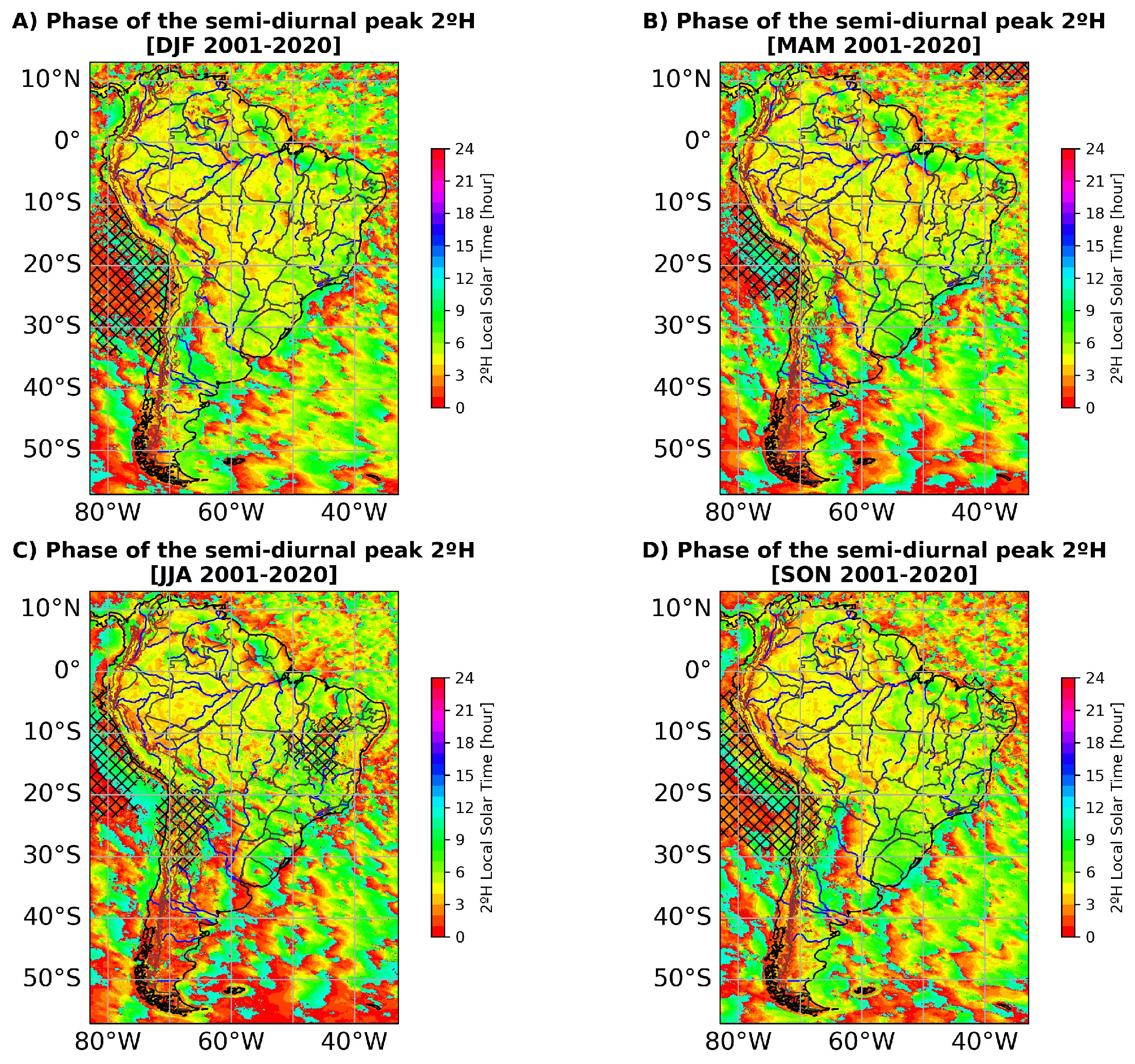
3.1. Climatology of the Diurnal Cycle of Precipitation
3.2. Regions with a Homogeneous Diurnal Cycle of Precipitation
3.3. Trends in the Diurnal Cycle of Precipitation
4. Discussion
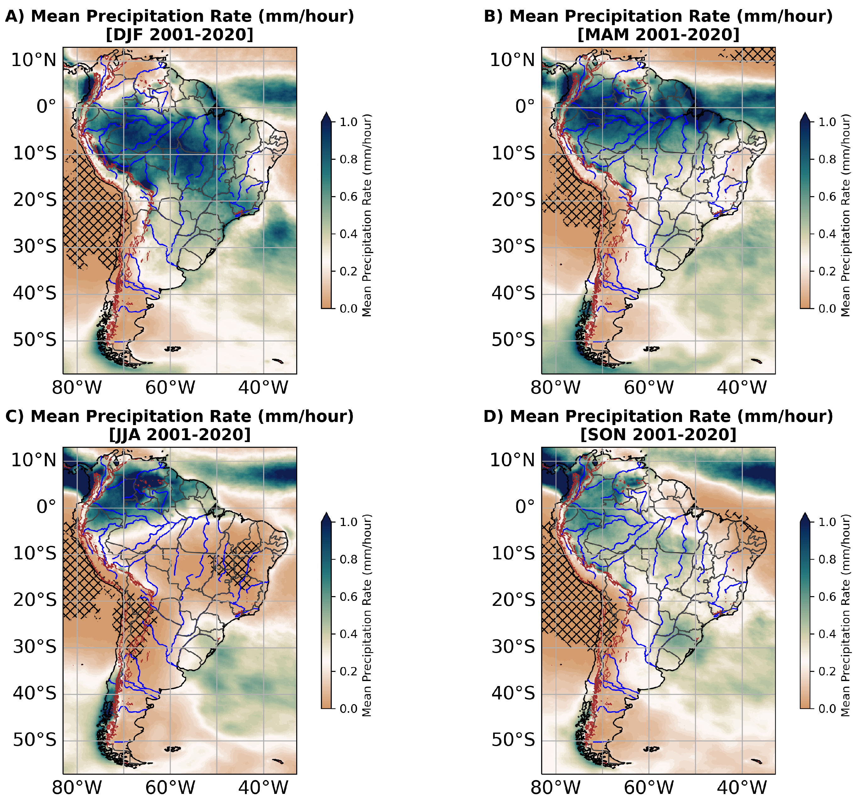
4.1. Mean Hourly Precipitation Rate
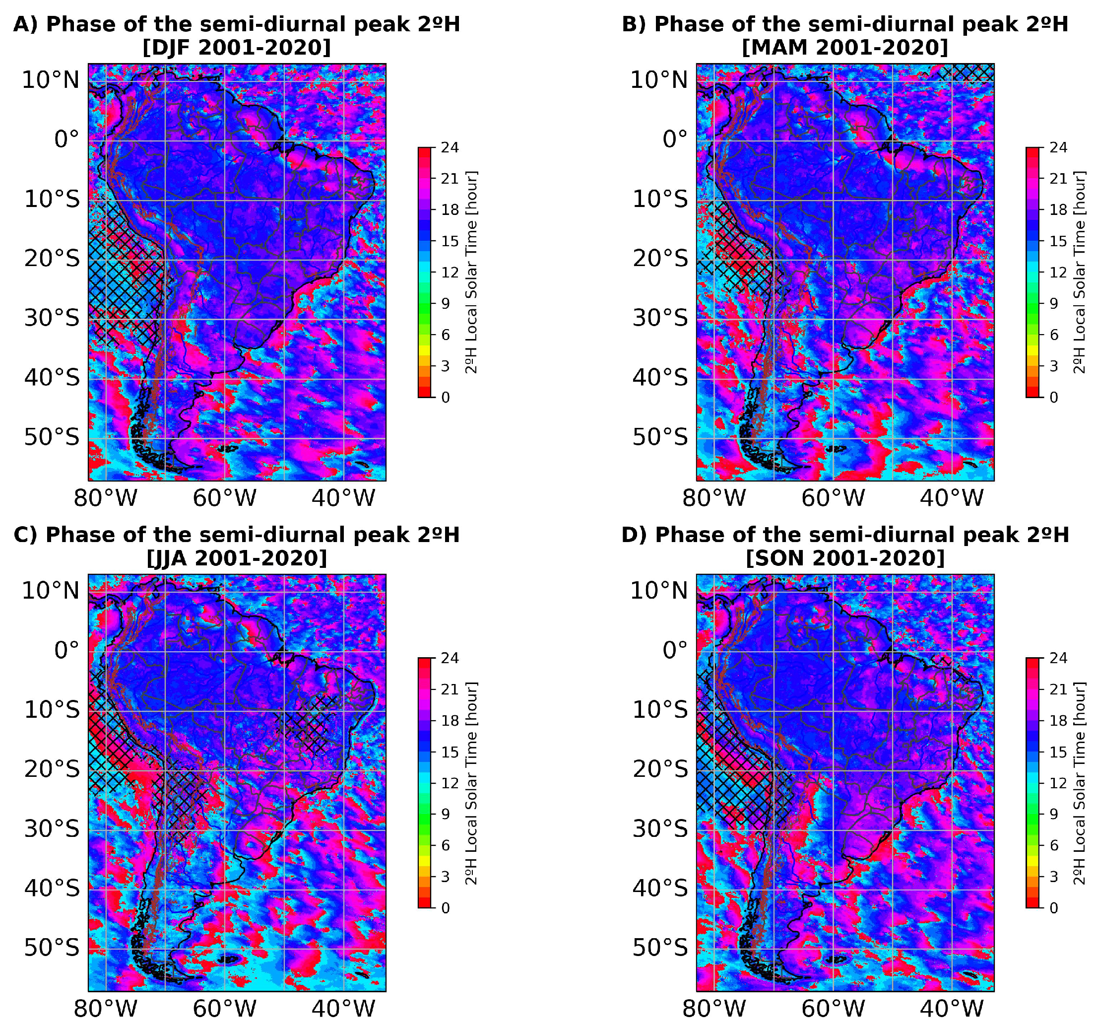
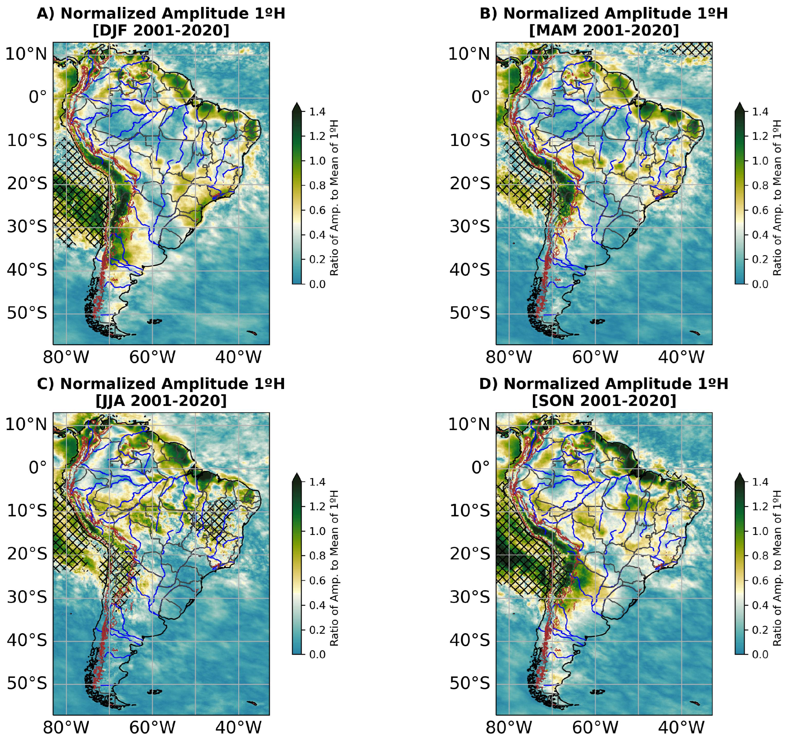
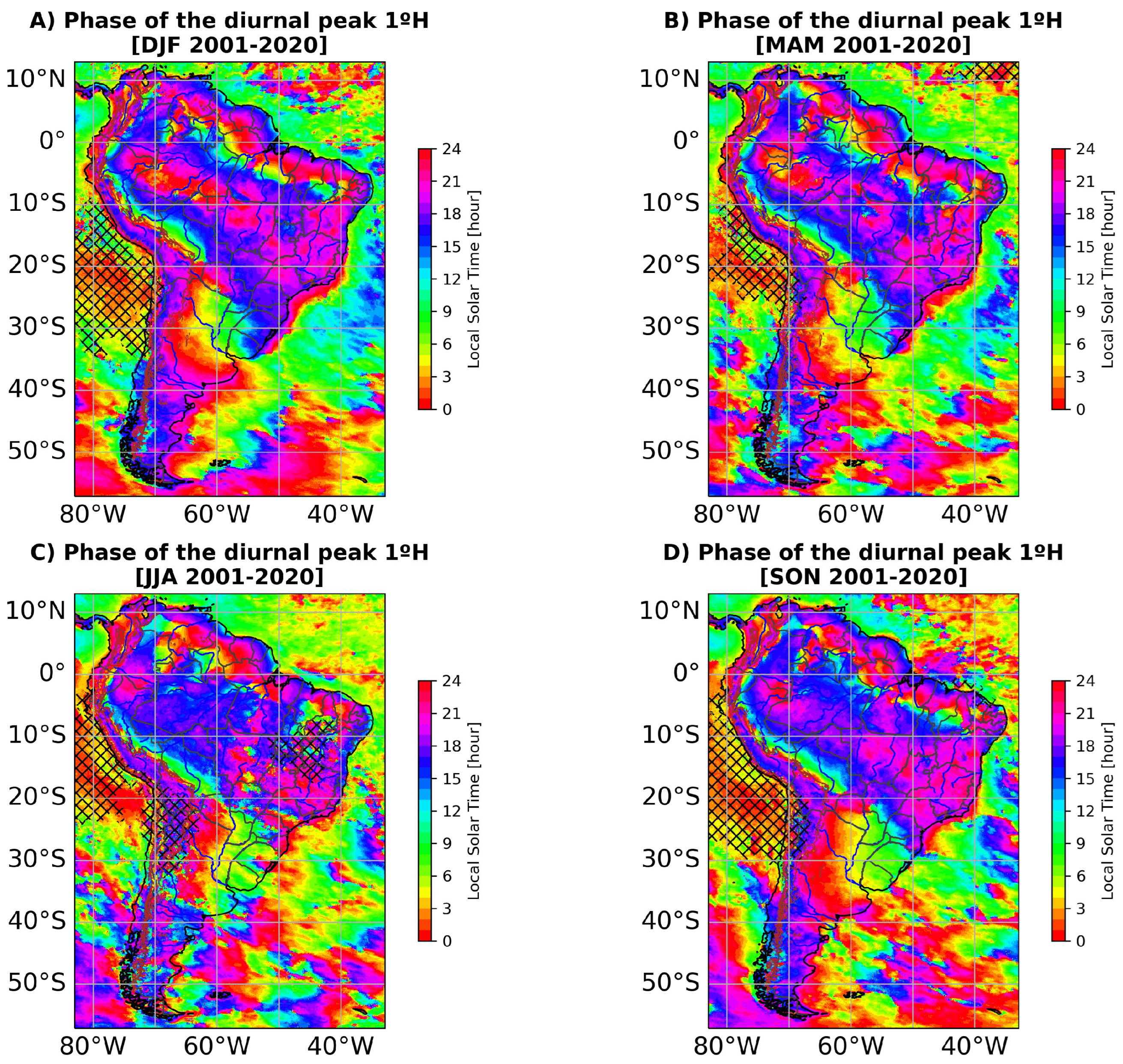
4.2. Normalized Amplitude and Phase of Scale-Diurnal Processes
4.3. Identification of Regions with a Homogeneous DCP
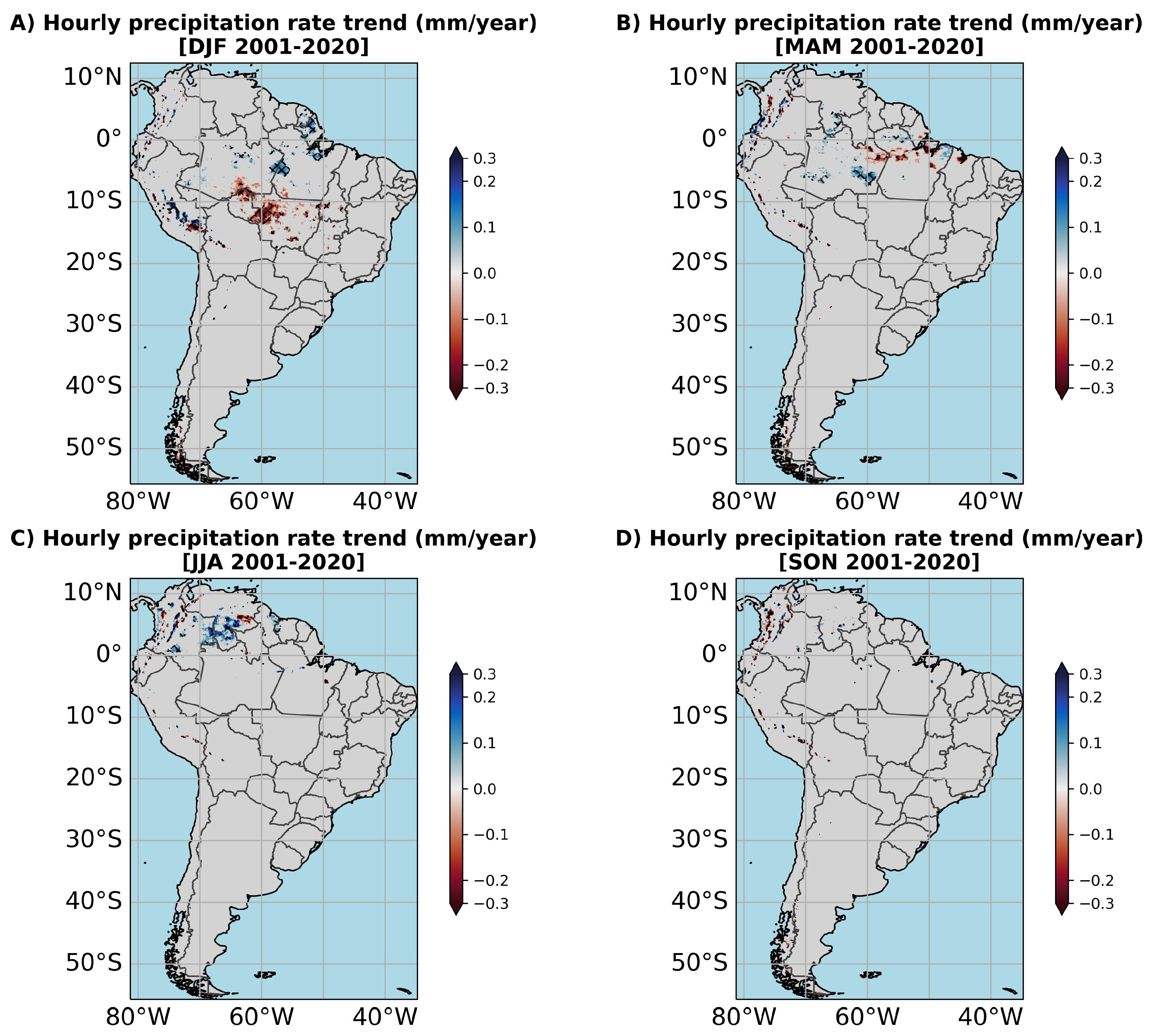
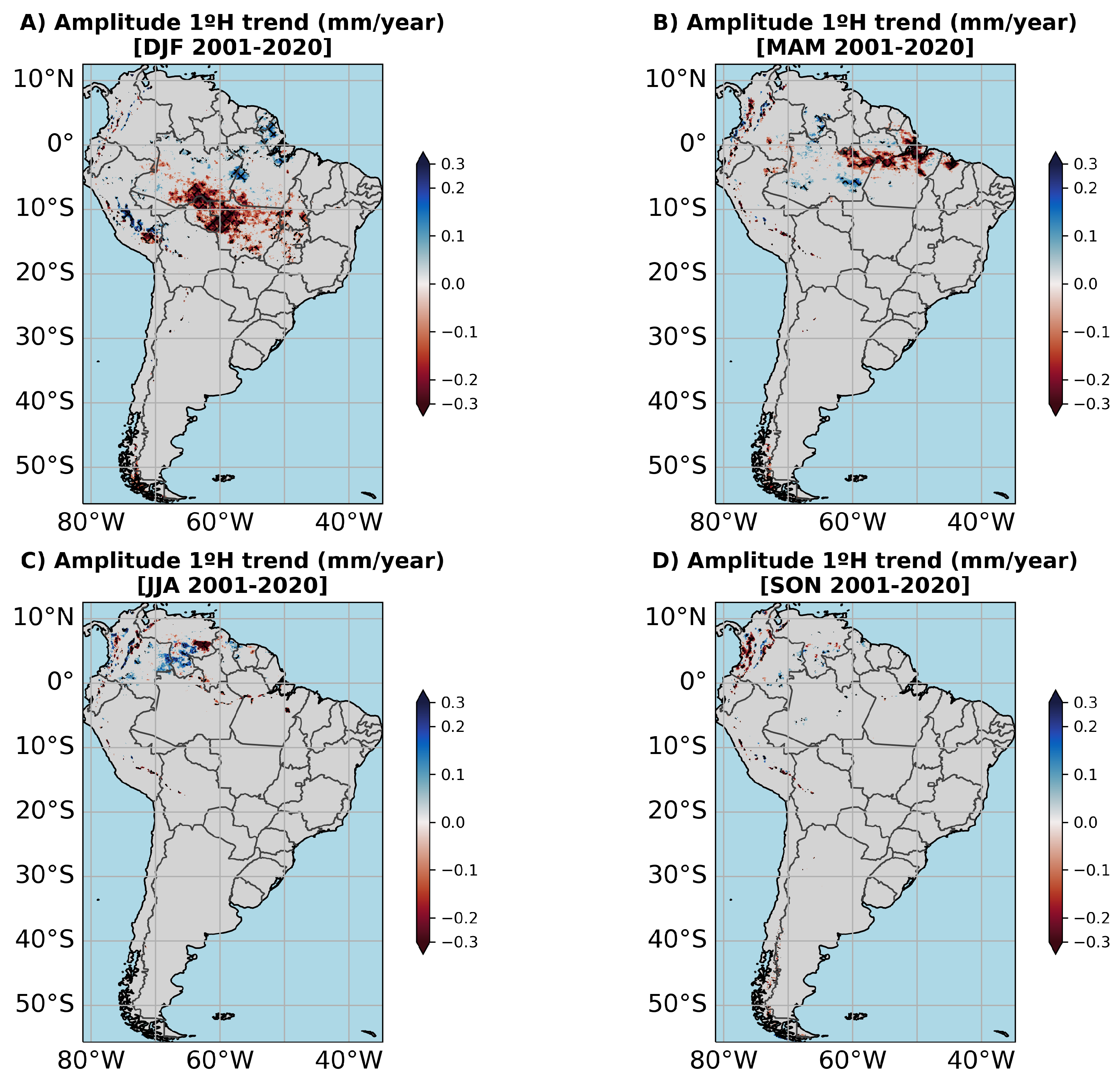
4.4. Historical Trends in the DCP
5. Summary and Conclusions
Supplementary Materials
Author Contributions
Funding
Institutional Review Board Statement
Informed Consent Statement
Data Availability Statement
Acknowledgments
Conflicts of Interest
Abbreviations
| Normalized Amplitude | |
| Normalized Amplitude of the second harmonic | |
| AB | Amazon Basin |
| ALLJ | Amazonian Low-Level Jet |
| CMIP5 | Coupled Model Intercomparison Project Phase 5 |
| CMIP6 | Coupled Model Intercomparison Project Phase 6 |
| DCP | Diurnal Cycle of Precipitation |
| DJF | December–January–February |
| ECMWF | European Centre for Medium-Range Weather Forecasts |
| EOF | Empirical Orthogonal Function |
| ENSO | El Niño-Southern Oscillation |
| ERA5 | ECMWF Reanalysis v5 |
| Mean precipitation rate | |
| GCM | General Circulation Model |
| GPM | Global Precipitation Measurement |
| IMERG | Integrated Multi-satellite Retrievals for the GPM |
| ITZC | Inter-Tropical Convergence Zone |
| JJA | June–July–August |
| LLJ | Low-Level Jets |
| LST | Local Solar Time |
| masl | meters above sea level |
| MAM | March–April–May |
| MCS | Mesoscale Convective System |
| MCSs | Mesoscale Convective Systems |
| MJO | Madden-Julian Oscillation |
| NESA | Northeastern South America |
| NWSA | Northwestern South America |
| PC | Principal Component |
| SA | South America |
| SACZ | South Atlantic Convergence Zone |
| SALLJ | South American Low-Level Jet |
| SAMS | South American Monsoon System |
| SESA | Southeastern South America |
| SLs | Squall Lines |
| SON | September–October–November |
| SSE | Sum of the Square Error |
| UTC | Coordinated Universal Time |
| Phase | |
| 1° H | First Harmonic |
| 2° H | Second Harmonic |
Appendix A
References
- Yang, G.Y.; Slingo, J. The diurnal cycle in the tropics. Mon. Weather. Rev. 2001, 129, 784. [Google Scholar] [CrossRef]
- Angelis, C.F.; McGregor, G.R.; Kidd, C. Diurnal cycle of rainfall over the Brazilian Amazon. Clim. Res. 2004, 26, 139. [Google Scholar] [CrossRef]
- Poveda, G.; Mesa, O.J.; Salazar, L.F.; Arias, P.A.; Moreno, H.A.; Vieira, S.C.; Agudelo, P.A.; Toro, V.G.; Alvarez, J.F. The diurnal cycle of precipitation in the tropical Andes of Colombia. Mon. Weather. Rev. 2005, 133, 228. [Google Scholar] [CrossRef]
- Tanaka, L.M.D.S.; Satyamurty, P.; Machado, L.A.T. Diurnal variation of precipitation in Central Amazon Basin. Int. J. Climatol. 2014, 34, 3574. [Google Scholar] [CrossRef]
- Junquas, C.; Takahashi, K.; Condom, T.; Espinoza, J.C.; Chávez, S.; Sicart, J.E.; Lebel, T. Understanding the influence of orography on the precipitation diurnal cycle and the associated atmospheric processes in the central Andes. Clim. Dyn. 2018, 50, 3995–4017. [Google Scholar] [CrossRef]
- Espinoza, J.C.; Garreaud, R.; Poveda, G.; Arias, P.A.; Molina-Carpio, J.; Masiokas, M.; Viale, M.; Scaff, L. Hydroclimate of the Andes Part I: Main Climatic Features. Front. Earth Sci. 2020, 8, 65. [Google Scholar] [CrossRef]
- Ruiz-Hernández, J.C.; Condom, T.; Ribstein, P.; Le Moine, N.; Espinoza, J.C.; Junquas, C.; Villacís, M.; Vera, A.; Muñoz, T.; Maisincho, L.; et al. Spatial variability of diurnal to seasonal cycles of precipitation from a high-altitude equatorial Andean valley to the Amazon Basin. J. Hydrol. Reg. Stud. 2021, 38, 100924. [Google Scholar] [CrossRef]
- Ramírez-Nina, R.G.; Silva Dias, M.A.F. Heterogeneity of the diurnal cycle of precipitation in the Amazon Basin. Front. Clim. 2024, 6, 1370097. [Google Scholar] [CrossRef]
- Betts, A.K.; Jakob, C. Study of diurnal cycle of convective precipitation over Amazonia using a single column model. J. Geophys. Res. Atmos. 2002, 107, 4732. [Google Scholar] [CrossRef]
- Dirmeyer, P.A.; Cash, B.A.; Kinter, J.L.; Shukla, J.; Pan, H.L.; Straus, D.M. Simulating the diurnal cycle of rainfall in global climate models: Resolution versus parameterization. Clim. Dyn. 2012, 39, 399–418. [Google Scholar] [CrossRef]
- Covey, C.; Gleckler, P.J.; Doutriaux, C.; Williams, D.N.; Dai, A.; Fasullo, J.; Trenberth, K.; Berg, A. Metrics for the diurnal cycle of precipitation: Toward routine benchmarks for climate models. J. Clim. 2016, 29, 4461–4471. [Google Scholar] [CrossRef]
- Watters, D.; Battaglia, A.; Allan, R.P. The diurnal cycle of precipitation according to multiple decades of global satellite observations, three CMIP6 models, and the ECMWF reanalysis. J. Clim. 2021, 34, 5063–5080. [Google Scholar] [CrossRef]
- Paccini, L.; Stevens, B. Assessing precipitation over the Amazon basin as simulated by a storm-resolving model. J. Geophys. Res. Atmos. 2023, 128, e2022JD037436. [Google Scholar] [CrossRef]
- Giles, J.A.; Ruscica, R.C.; Menéndez, C.G. The diurnal cycle of precipitation over South America represented by five gridded datasets. Int. J. Climatol. 2020, 40, 668–686. [Google Scholar] [CrossRef]
- da Rocha, R.P.; Llopart, M.; Reboita, M.S.; Silva, L.C.; Silva, A.P.; Carrasco, G.G. Precipitation Diurnal Cycle Assessment in Convection-Permitting Simulations in Southeastern South America. Earth Syst. Environ. 2024, 8, 1–19. [Google Scholar] [CrossRef]
- Hersbach, H.; Bell, B.; Berrisford, P.; Hirahara, S.; Horányi, A.; Muñoz-Sabater, J.; Nicolas, J.; Peubey, C.; Radu, R.; Schepers, D.; et al. The ERA5 global reanalysis. Q. J. R. Meteorol. Soc. 2020, 146, 1999–2049. [Google Scholar] [CrossRef]
- Saraiva, I.; Dias, M.A.F.S.; Morales, C.A.R.; Saraiva, J.M.B. Regional Variability of Rain Clouds in the Amazon Basin as Seen by a Network of Weather Radars. J. Appl. Meteorol. Climatol. 2016, 55, 2657–2676. [Google Scholar] [CrossRef]
- Chavez, S.P.; Silva, Y.; Barros, A.P. High-elevation Monsoon Precipitation Processes in the Central Andes of Peru. J. Geophys. Res. Atmos. 2020, 125, e2020JD032947. [Google Scholar] [CrossRef]
- Bedoya-Soto, J.M.; Aristizábal, E.; Carmona, A.M.; Poveda, G. Seasonal Shift of the Diurnal Cycle of Rainfall Over Medellin’s Valley, Central Andes of Colombia (1998–2005). Front. Earth Sci. 2019, 7, 92. [Google Scholar] [CrossRef]
- Bendix, J.; Rollenbeck, R.; Reudenbach, C. Diurnal Patterns of Rainfall in a Tropical Andean Valley of Southern Ecuador as Seen by a Vertically Pointing K-band Doppler Radar. Int. J. Climatol. 2006, 26, 829–846. [Google Scholar] [CrossRef]
- Watters, D.; Battaglia, A. The summertime diurnal cycle of precipitation derived from IMERG. Remote Sens. 2019, 11, 1781. [Google Scholar] [CrossRef]
- Tan, J.; Petersen, W.A.; Tokay, A. A Novel Approach to Identify Sources of Errors in IMERG for GPM Ground Validation. J. Hydrometeorol. 2016, 17, 2477–2491. [Google Scholar] [CrossRef]
- Gadelha, A.N.; Coelho, V.H.R.; Xavier, A.C.; Barbosa, L.R.; Melo, D.C.D.; Xuan, Y.; Huffman, G.J.; Petersen, W.A.; Almeida, C.d.N. Grid box-level evaluation of IMERG over Brazil at various space and time scales. Atmos. Res. 2019, 218, 231–244. [Google Scholar] [CrossRef]
- Tapiador, F.J.; Navarro, A.; García-Ortega, E.; Merino, A.; Sánchez, J.L.; Marcos, C.; Kummerow, C. The Contribution of Rain Gauges in the Calibration of the IMERG Product: Results from the First Validation over Spain. J. Hydrometeorol. 2020, 21, 161–182. [Google Scholar] [CrossRef]
- Pradhan, R.K.; Markonis, Y.; Godoy, M.R.V.; Villalba-Pradas, A.; Andreadis, K.M.; Nikolopoulos, E.I.; Papalexiou, S.M.; Rahim, A.; Tapiador, F.J.; Hanel, M. Review of GPM IMERG performance: A global perspective. Remote Sens. Environ. 2022, 268, 112754. [Google Scholar] [CrossRef]
- Dai, A.; Lin, X.; Hsu, K.L. The Frequency, Intensity, and Diurnal Cycle of Precipitation in Surface and Satellite Observations over Low- and Mid-Latitudes. Clim. Dyn. 2007, 29, 727–744. [Google Scholar] [CrossRef]
- Zhou, J.; Lau, K.M. Does a Monsoon Climate Exist over South America? J. Clim. 1998, 11, 1020–1040. [Google Scholar] [CrossRef]
- Carvalho, L.M.; Jones, C.; Silva, A.E.; Liebmann, B.; Silva, D.P. The South American Monsoon System and the 1970s Climate Transition. Int. J. Climatol. 2011, 31, 1248. [Google Scholar] [CrossRef]
- Vera, C.; Higgins, W.; Amador, J.; Ambrizzi, T.; Garreaud, R.; Gochis, D.; Gutzler, D.; Lettenmaier, D.; Marengo, J.; Mechoso, C.R.; et al. Toward a unified view of the American monsoon systems. J. Clim. 2006, 19, 4977–5000. [Google Scholar] [CrossRef]
- Marengo, J.A.; Liebmann, B.; Grimm, A.M.; Misra, V.; Silva Dias, P.L.; Cavalcanti, I.F.A.; Carvalho, L.M.V.; Berbery, E.H.; Ambrizzi, T.; Vera, C.S.; et al. Recent developments on the South American monsoon system. Int. J. Climatol. 2012, 32, 1–21. [Google Scholar] [CrossRef]
- Grimm, A.M.; Dominguez, F.; Cavalcanti, I.F.; Cavazos, T.; Gan, M.A.; Silva Dias, P.L.; Fu, R.; Castro, C.; Hu, H.; Barreiro, M. South and North American Monsoons: Characteristics, life cycle, variability, modeling, and prediction. In The Multiscale Global Monsoon System; World Scientific: Singapore, 2020; pp. 49–66. [Google Scholar]
- Chavez, S.P.; Takahashi, K. Orographic rainfall hot spots in the Andes-Amazon transition according to the TRMM precipitation radar and in situ data. J. Geophys. Res. Atmos. 2017, 122, 5870–5882. [Google Scholar] [CrossRef]
- Espinoza, J.C.; Chavez, S.; Ronchail, J.; Junquas, C.; Takahashi, K.; Lavado, W. Rainfall hotspots over the southern tropical Andes: Spatial distribution, rainfall intensity, and relations with large-scale atmospheric circulation. Water Resour. Res. 2015, 51, 3459–3475. [Google Scholar] [CrossRef]
- Espinoza, J.C.; Ronchail, J.; Guyot, J.L.; Cochonneau, G.; Naziano, F.; Lavado, W.; De Oliveira, E.; Pombosa, R.; Vauchel, P. Spatio-temporal rainfall variability in the Amazon basin countries (Brazil, Peru, Bolivia, Colombia, and Ecuador). Int. J. Climatol. 2009, 29, 1574. [Google Scholar] [CrossRef]
- Albrecht, R.I.; Goodman, S.J.; Buechler, D.E.; Blakeslee, R.J.; Christian, H.J. Where Are the Lightning Hotspots on Earth? Bull. Am. Meteorol. Soc. 2016, 97, 2051–2068. [Google Scholar] [CrossRef]
- Huffman, G.J.; Stocker, E.F.; Bolvin, D.T.; Nelkin, E.J.; Tan, J. GPM IMERG Final Precipitation L3 Half Hourly 0.1 Degree x 0.1 Degree V06. 2019. Available online: https://disc.gsfc.nasa.gov/datasets/GPM_3IMERGHH_07/summary (accessed on 1 November 2021).
- Huffman, G.; Braithwaite, D.; Hsu, K.; Joyce, R.; Kidd, C.; Nelkin, E.; Sorooshian, S.; Stocker, E.F.; Tan, J.; Wolff, D.B. Integrated Multi-satellite Retrievals for the Global Precipitation Measurement (GPM) Mission (IMERG). In Satellite Precipitation Measurement; Levizzani, V., Kidd, C., Kirschbaum, D.B., Kummerow, C.D., Nakamura, K., Turk, F.J., Eds.; Advances in Global Change Research; Springer: Cham, Switzerland, 2020; Volume 67. [Google Scholar] [CrossRef]
- Tan, J.; Huffman, G.J.; Bolvin, D.T.; Nelkin, E.J. Diurnal cycle of IMERG V06 precipitation. Geophys. Res. Lett. 2019, 46, 13584–13592. [Google Scholar] [CrossRef]
- Dominguez, F.; Rasmussen, R.; Liu, C.; Ikeda, K.; Prein, A.; Varble, A.; Arias, P.A.; Bacmeister, J.; Bettolli, M.L.; Callaghan, P.; et al. Advancing South American Water and Climate Science through Multidecadal Convection-Permitting Modeling. Bull. Am. Meteorol. Soc. 2024, 105, E32–E44. [Google Scholar] [CrossRef]
- Rehbein, A.; Ambrizzi, T. Mesoscale convective systems over the Amazon basin in a changing climate under global warming. Clim. Dyn. 2023, 61, 1815–1827. [Google Scholar] [CrossRef]
- Rehbein, A.; Ambrizzi, T.; Mechoso, C.R.; Espinosa, S.A.; Myers, T.A. Mesoscale convective systems over the Amazon basin: The GoAmazon2014/5 program. Int. J. Climatol. 2019, 39, 5599–5618. [Google Scholar] [CrossRef]
- Nesbitt, S.W.; Cifelli, R.; Rutledge, S.A. Storm morphology and rainfall characteristics of TRMM precipitation features. Mon. Weather. Rev. 2006, 134, 2702. [Google Scholar] [CrossRef]
- Wilks, D.S. Statistical Methods in the Atmospheric Sciences, 3rd ed.; International Geophysics Series; Academic Press: Oxford, UK, 2011; Volume 100. [Google Scholar]
- Easterling, D.R.; Robinson, P.J. The diurnal variation of thunderstorm activity in the United States. J. Appl. Meteorol. Climatol. 1985, 24, 1048–1058. [Google Scholar] [CrossRef]
- Lorenz, E.N. Empirical Orthogonal Functions and Statistical Weather Prediction; Massachusetts Institute of Technology, Department of Meteorology: Cambridge, UK, 1956; Volume 1. [Google Scholar]
- Van Der Maaten, L.; Postma, E.O.; Van Den Herik, H.J. Dimensionality reduction: A comparative review. J. Mach. Learn. Res. 2009, 10, 13. [Google Scholar]
- Mann, H.B. Nonparametric Tests Against Trend. Econometrica 1945, 13, 245–259. [Google Scholar] [CrossRef]
- Kendall, K. Thin-Film Peeling—The Elastic Term. J. Phys. D Appl. Phys. 1975, 8, 1449–1452. [Google Scholar] [CrossRef]
- Sen, P.K. Estimates of the Regression Coefficient Based on Kendall’s Tau. J. Am. Stat. Assoc. 1968, 63, 1379–1389. [Google Scholar] [CrossRef]
- Cohen, J.C.; Silva Dias, M.A.; Nobre, C.A. Environmental conditions associated with Amazonian squall lines: A case study. Mon. Weather. Rev. 1995, 123, 3163. [Google Scholar] [CrossRef]
- Alcântara, C.R.; Dias, M.A.S.; Souza, E.P.; Cohen, J.C. Verification of the role of the low level jets in Amazon squall lines. Atmos. Res. 2011, 100, 36. [Google Scholar] [CrossRef]
- Horel, J.D.; Hahmann, A.N.; Geisler, J.E. An investigation of the annual cycle of convective activity over the tropical Americas. J. Clim. 1989, 2, 1388–1403. [Google Scholar] [CrossRef]
- Marengo, J.A.; Soares, W.R.; Saulo, C.; Nicolini, M. Climatology of the low-level jet east of the Andes as derived from the NCEP–NCAR reanalyses: Characteristics and temporal variability. J. Clim. 2004, 17, 2261. [Google Scholar] [CrossRef]
- Liebmann, B.; Kiladis, G.N.; Vera, C.S.; Saulo, A.C.; Carvalho, L.M.V. Subseasonal Variations of Rainfall in South America in the Vicinity of the Low-Level Jet East of the Andes and Comparison to Those in the South Atlantic Convergence Zone. J. Clim. 2004, 17, 3829–3842. [Google Scholar] [CrossRef]
- Salio, P.; Nicolini, M.; Zipser, E.J. Mesoscale Convective Systems over Southeastern South America and Their Relationship with the South American Low-Level Jet. Mon. Weather. Rev. 2007, 135, 1290–1309. [Google Scholar] [CrossRef]
- Arraut, J.M.; Nobre, C.; Barbosa, H.M.; Obregon, G.; Marengo, J. Aerial rivers and lakes: Looking at large-scale moisture transport and its relation to Amazonia and to subtropical rainfall in South America. J. Clim. 2012, 25, 543. [Google Scholar] [CrossRef]
- Drumond, A.; Marengo, J.; Ambrizzi, T.; Nieto, R.; Moreira, L.; Gimeno, L. The role of the Amazon Basin moisture in the atmospheric branch of the hydrological cycle: A Lagrangian analysis. Hydrol. Earth Syst. Sci. 2014, 18, 2577–2598. [Google Scholar] [CrossRef]
- Jones, C.; Mu, Y.; Carvalho, L.M.V.; Ding, Q. The South America Low-Level Jet: Form, variability and large-scale forcings. NPJ Clim. Atmos. Sci. 2023, 6, 175. [Google Scholar] [CrossRef]
- Poveda, G. La hidroclimatología de Colombia: Una síntesis desde la escala inter-decadal hasta la escala diurna. Rev. Acad. Colomb. Cienc. Exactas Físicas Nat. 2004, 28, 201–222. [Google Scholar] [CrossRef]
- Rehbein, A.; Ambrizzi, T.; Mechoso, C.R. Mesoscale convective systems over the Amazon basin. Part I: Climatological aspects. Int. J. Climatol. 2017, 38, 215–229. [Google Scholar] [CrossRef]
- Rehbein, A. Sistemas Convectivos de Mesoescala na Bacia Amazônica: Clima Presente e ProjeçõEs Futuras em Cenários de MudançAs ClimáTicas. Ph.D. Thesis, Instituto de Astronomia, Geofísica e Ciências Atmosféricas, Universidade de São Paulo, São Paulo, Brazil, 2021. [Google Scholar] [CrossRef]
- Teodoro, T.A.; Reboita, M.S.; Llopart, M.; da Rocha, R.P.; Ashfaq, M. Climate change impacts on the South American Monsoon System and its surface–atmosphere processes through RegCM4 CORDEX-CORE projections. Earth Syst. Environ. 2021, 5, 825–847. [Google Scholar] [CrossRef]
- Satyamurty, P.; Nobre, C.A.; Silva, D.P. Meteorology of the Southern Hemisphere; Springer: Berlin/Heidelberg, Germany; American Meteorological Society: Boston, MA, USA, 1998; pp. 119–139. [Google Scholar]
- Cai, W.; McPhaden, M.J.; Grimm, A.M.; Rodrigues, R.R.; Taschetto, A.S.; Garreaud, R.D.; Dewitte, B.; Poveda, G.; Ham, Y.G.; Santoso, A.; et al. Climate impacts of the El Niño–Southern Oscillation on South America. Nat. Rev. Earth Environ. 2020, 1, 215–231. [Google Scholar] [CrossRef]
- Reboita, M.S.; Gan, M.A.; Porfírio, R.; Rocha, D.A.; Ambrizzi, T. Regimes de precipitação na América do Sul: Uma revisão bibliográfica. Rev. Bras. Meteorol. 2010, 25, 185–204. [Google Scholar] [CrossRef]
- Poveda, G.; Waylen, P.R.; Pulwarty, R.S. Annual and inter-annual variability of the present climate in northern South America and southern Mesoamerica. Palaeogeogr. Palaeoclimatol. Palaeoecol. 2006, 234, 3–27. [Google Scholar] [CrossRef]
- Gimeno, L.; Dominguez, F.; Nieto, R.; Trigo, R.; Drumond, A.; Reason, C.; Taschetto, A.; Ramos, A.; Kumar, R.; Marengo, J. Major Mechanisms of Atmospheric Moisture Transport and Their Role in Extreme Precipitation Events. Annu. Rev. Environ. Resour. 2016, 41, 117–141. [Google Scholar] [CrossRef]
- Viale, M.; Valenzuela, R.; Garreaud, R.D.; Ralph, F.M. Impacts of Atmospheric Rivers on Precipitation in Southern South America. J. Hydrometeorol. 2018, 19, 1671–1687. [Google Scholar] [CrossRef]
- Anselmo, E.M.; Machado, L.A.T.; Schumacher, C.; Kiladis, G.N. Amazonian mesoscale convective systems: Life cycle and propagation characteristics. Int. J. Climatol. 2021, 41, 3968–3981. [Google Scholar] [CrossRef]
- Anselmo, E.M.; Schumacher, C.; Machado, L.A. The Amazonian low-level jet and its connection to convective cloud propagation and evolution. Mon. Weather. Rev. 2020, 148, 4083. [Google Scholar] [CrossRef]
- Bendix, J.; Rollenbeck, R.; Göttlicher, D.; Cermák, J. Cloud occurrence and cloud properties in Ecuador. Clim. Res. 2006, 30, 133–147. [Google Scholar] [CrossRef]
- Torrealba, E.; Amador, J. La corriente en chorro de bajo nivel sobre los Llanos Venezolanos de Sur América. Rev. Climatol. 2010, 10, 1–20. [Google Scholar]
- Silva Dias, M.; Silva Dias, P.; Longo, M.; Fitzjarrald, D.R.; Denning, A.S. River breeze circulation in eastern Amazonia: Observations and modelling results. Theor. Appl. Climatol. 2004, 78, 111–121. [Google Scholar] [CrossRef]
- dos Santos, M.J.; Silva Dias, M.A.; Freitas, E.D. Influence of local circulations on wind, moisture, and precipitation close to Manaus City, Amazon Region, Brazil. J. Geophys. Res. Atmos. 2014, 119, 13–233. [Google Scholar] [CrossRef]
- Santos, M.J.; Medvigy, D.; Silva Dias, M.A.; Freitas, E.D.; Kim, H. Seasonal flooding causes intensification of the river breeze in the Central Amazon. J. Geophys. Res. Atmos. 2019, 124, 5178. [Google Scholar] [CrossRef]
- Silva Dias, M.A.F.; Petersen, W.; Silva Dias, P.L.; Cifelli, R.; Betts, A.K.; Longo, M.; Gomes, A.M.; Fisch, G.F.; Lima, M.A.; Antonio, M.A.; et al. A case study of convective organization into precipitating lines in the Southwest Amazon during the WETAMC and TRMM-LBA. J. Geophys. Res. Atmos. 2002, 107, LBA 46-1–LBA 46-15. [Google Scholar] [CrossRef]
- Carvalho, L.M.; Jones, C.; Silva, D.M. Intraseasonal large-scale circulations and mesoscale convective activity in tropical South America during the TRMM-LBA campaign. J. Geophys. Res. Atmos. 2002, 107, 1–9. [Google Scholar] [CrossRef]
- Carvalho, L.M.V.; Jones, C.; Liebmann, B. The South Atlantic Convergence Zone: Intensity, Form, Persistence, and Relationships with Intraseasonal to Interannual Activity and Extreme Rainfall. J. Clim. 2004, 17, 88–108. [Google Scholar] [CrossRef]
- Vera, C.; Baez, J.; Douglas, M.; Emmanuel, C.B.; Marengo, J.; Meitin, J.; Nicolini, M.; Nogues-Paegle, J.; Paegle, J.; Penalba, O.; et al. The South American Low-Level Jet Experiment. Bull. Am. Meteorol. Soc. 2006, 87, 63–78. [Google Scholar] [CrossRef]
- Assunção, R.M.; Neves, M.C.; Câmara, G.; Da Costa Freitas, C. Efficient Regionalization Techniques for Socio-Economic Geographical Units Using Minimum Spanning Trees. Int. J. Geogr. Inf. Sci. 2006, 20, 797–811. [Google Scholar] [CrossRef]
- De la Cruz, G.; Huerta, A.; Espinoza, J.C.; Lavado-Casimiro, W. Present Variability and Future Change in Onset and Cessation of the Rainy Season Over Peru. Int. J. Climatol. 2025, 45, e8700. [Google Scholar] [CrossRef]
- Espinoza, J.C.; Ronchail, J.; Marengo, J.A.; Segura, H. Contrasting north–south changes in Amazon wet-day and dry-day frequency and related atmospheric features (1981–2017). Clim. Dyn. 2019, 52, 5413–5430. [Google Scholar] [CrossRef]
- Cerón, W.L.; Kayano, M.T.; Andreoli, R.V.; Canchala, T.; Avila-Diaz, A.; Ribeiro, I.O.; Rojas, J.D.; Escobar-Carbonari, D.; Tapasco, J. New insights into trends of rainfall extremes in the Amazon basin through trend-empirical orthogonal function (1981–2021). Int. J. Climatol. 2024, 44, 3955–3975. [Google Scholar] [CrossRef]
- Nobre, C.A.; Sellers, P.J.; Shukla, J. Amazonian deforestation and regional climate change. J. Clim. 1991, 4, 957–988. [Google Scholar] [CrossRef]
- Silva Dias, M.A.F.; Rutledge, S.; Kabat, P.; Silva Dias, P.L.; Nobre, C.; Fisch, G.; Dolman, A.J.; Zipser, E.; Garstang, M.; Manzi, A.O.; et al. Cloud and rain processes in a biosphere–atmosphere interaction context in the Amazon region. J. Geophys. Res. Atmos. 2002, 107, LBA 39-1–LBA 39-18. [Google Scholar] [CrossRef]
- Debortoli, N.S.; Dubreuil, V.; Funatsu, B.; Delahaye, F.; de Oliveira, C.H.; Rodrigues-Filho, S.; Saito, C.H.; Fetter, R. Rainfall patterns in the Southern Amazon: A chronological perspective (1971–2010). Clim. Change 2015, 132, 251–264. [Google Scholar] [CrossRef]
- Artaxo, P.; Rizzo, L.V.; Brito, J.F.; Barbosa, H.M.J.; Arana, A.; Sena, E.T.; Cirino, G.G.; Bastos, W.; Martin, S.T.; Andreae, M.O. Atmospheric aerosols in Amazonia and land use change: From natural biogenic to biomass burning conditions. Faraday Discuss. 2013, 165, 203–235. [Google Scholar] [CrossRef]


| Season | Cluster | Precipitation Rate (mm/h) | Phase () | Geographic Location | |
|---|---|---|---|---|---|
| DJF | 1 | >0.254 | >0.5 (U) | morning | Hotspots regions of Peru and Bolivia; eastern side of the central Andes in Peru; Amazon region of Ecuador; coast of Colombia; and Amazonian rivers in Brazil. |
| 2 | ≈0.254 | <0.5 (B) | late afternoon–evening | Paraguay; SE of Brazil; Southern Argentina; NW of SA (Ecuador, Colombia and Venezuela). | |
| 3 | <0.254 | >0.5 (U) | afternoon–night | Northeasternmost region, extreme north, Western region of SA (Argentina, Bolivia, Chile and Peru). | |
| 4 | ≈0.4 | <0.5 (B) | afternoon, dawn | SE of SA (NE of Argentina, SE of Brazil and Uruguay); NE of Bolivia; Peruvian, Ecuadorian and Colombian Amazon; northern and Northeastern Brazil; Southern Argentina and Chile. | |
| 5 | >0.254 | >0.5 (U) | afternoon–night | NE-SA; SE-Brazil; coastal region of Colombia; some inland regions. | |
| 6 | >0.254 | <0.5 (B) | night–dawn, afternoon | Tropical region of SA (in the AB) with a northwest-southeast-oriented configuration. | |
| 7 | >0.254 | <0.5 (B) | night–dawn, afternoon | Tropical region of SA (inside the AB) with a northwest-southeast-oriented configuration; NE Argentina. | |
| 8 | ≈0.254 | >0.5 (U) | nightime | Argentina; Ecuador; NE and N of Brazil; Southern Guyana; Venezuela; highland of Colombia; and northern Peru. | |
| MAM | 1 | >0.254 | >0.5 (U) | afternoon–evening | Along the western and eastern coasts of SA |
| 2 | ≈0.6 | <0.5 (B) | early morning, afternoon | AB (north of 10° S). | |
| 3 | 0.4 mm/h; <0.254 (S. Argentina) | <0.5 (B) | afternoon–evening, morning | Northern Uruguay; Southern, Western Center and Northeastern Brazil; Southern Chile and Argentina; Venezuela; and northern highlands of Peru. | |
| 4 | ≈0.4 | >0.5 (U) | dawn–morning | In region with altitudes ranging from 600 to 1500 masl; hotspot regions of Peru and Bolivia and area of intense precipitation gradient located along the eastern slopes of the Central Andes in Peru. | |
| 5 | ≈0.254 | <0.5 (B) | afternoon–evening, morning | Highland of Ecuador and Peru; Southern and Central Argentina; Southern and Central Chile; Southern, Northeastern, and Western Center Brazil; and some regions in the extreme north of SA. | |
| 6 | <0.254 | >0.5 (U) | afternoon–evening | Along the western and eastern coasts of SA. | |
| 7 | ≈0.6 | <0.5 (B) | afternoon–evening, early morning | AB (north of 10 S ); southernmost of SA (Southern Chile). | |
| 8 | ≈0.4 | <0.5 (B) | early morning–morning, late afternoon | SE of SA (Northern and Northeastern Argentina, Southern Uruguay); Paraguay; Bolivia; Peru; Southern Argentina; North and Northeastern Brazil; Venezuela. | |
| JJA | 1 | <0.254 | <0.5 (B) | early morning–morning, afternoon | Subtropical region and mid-latitudes (Argentina). |
| 2 | >0.254 (N. equator); <0.254 (S. equator) | >0.5 (U) | afternoon | Tropical region of SA (near 10 S—including highest elevations of the tropical Andes in Bolivia and Peru, coastal region on the eastern side of SA). | |
| 3 | >0.6 (north of 5° S); <0.254 (south of 5° S) | <0.5 (B) | afternoon–evening, early morning–morning | Brazilian, Colombian, Ecuadorian, and Peruvian Amazon; parts of Venezuela; some regions of Southeastern Brazil. | |
| 4 | >0.6 (N. equator); <0.254 (S. equator) | >0.5 (U) | nighttime–dawn | Tropical region of SA (along the coastal regions of Colombia and Ecuador, over tropical Andes of Bolivia and Peru–above 1500 masl—, and a few hundred kilometers inland from the coast in the northern and northeastern regions of SA). | |
| 5 | >0.8 (N. equator); <0.254 (S. equator) | >0.5 (U) | late dawn–morning | Tropical region of SA (Colombia, some regions in Ecuador, Bolivia and Peru—covering precipitation hotspots below 1500 masl); Northern Argentina; a few kilometers inland from the eastern coast of SA. | |
| 6 | <0.254 | <0.5 (B) | morning, evening | Southeastern Brazil; Paraguay; and Southern Argentina. | |
| 7 | >0.254 | <0.5 (B) | morning, night-to-dawn | Southeastern region of SA (Southeastern Brazil, Uruguay, and Northeastern Argentina); Paraguay. | |
| 8 | <0.254 | <0.5 (B) | noisy signal | Southern Argentina; Southern Chile. | |
| SON | 1 | ≈0.6 | <0.5 (B) | afternoon, morning | SE of SA. |
| 2 | <0.254 (Andean Mountains and near the eastern coast of SA); >0.254 (along the northern coast of the continent and over the AB) | >0.5 (U) | afternoon–evening | High elevations of the Andean Mountain; a few hundred kilometers inland from the northeastern coast of SA; along the northern coast of the continent; over the AB. | |
| 3 | >0.254 (Amazon and SE. Brazil); <0.254 (E. Brazil, and Argentina) | <0.5 (B) | night-to-morning, afternoon | Southeastern and Eastern Brazil; Brazilian and Peruvian Amazon; central region of Argentina. | |
| 4 | ≈0.254 (S. equator); >0.254 (N. equator) | >0.5 (U) | night-to-early morning | Venezuela (near Lake Maracaibo); Colombia near the Andes; Southern Paraguay; Northern Argentina. | |
| 5 | >0.254 | <0.5 (B) | late dawn–morning, late afternoon–evening | Scattered across several regions of SA (including the precipitation hotspots regions); eastern side of the Central and Northern Andes of Peru; Northeastern Argentina; Ecuador; Colombia; and the Brazilian Amazon. | |
| 6 | >0.254 (in the AB); <0.254 (in the others areas) | >0.5 (U) | afternoon | Andean region (above 1500 m a.s.l.) of Bolivia and Peru; along the northern and northeastern coast of SA; in the AB; and some portions of Argentina. | |
| 7 | <0.254 | >0.5 (U) | night | A few hundred kilometers inland from the northeastern and northern coasts of SA; Ecuador, Colombia; and the mountains region of Northwestern Argentina. | |
| 8 | >0.254 (Amazonian regions, Ecuador, Colombia and Venezuela); <0.254 (in the other regions) | <0.5 (B) | afternoon, early morning | Southern Argentina; Central and Southern Chile; Peru (in the northern part of the Andes and its Amazon region); the Brazilian Amazon; and along the northeastern coast of Brazil, Ecuador Colombia and Venezuela. | |
| 9 | >0.254 (Northeastern Argentina, and Colombia); <0.254 (in the other regions) | >0.5 (U) | dawn–morning | Northwest (parallel to the Andes configuration) and northeast of Argentina; the interior of Northeastern Brazil; and Colombia. |
Disclaimer/Publisher’s Note: The statements, opinions and data contained in all publications are solely those of the individual author(s) and contributor(s) and not of MDPI and/or the editor(s). MDPI and/or the editor(s) disclaim responsibility for any injury to people or property resulting from any ideas, methods, instructions or products referred to in the content. |
© 2025 by the authors. Licensee MDPI, Basel, Switzerland. This article is an open access article distributed under the terms and conditions of the Creative Commons Attribution (CC BY) license (https://creativecommons.org/licenses/by/4.0/).
Share and Cite
Ramírez-Nina, R.G.; da Silva Dias, M.A.F.; da Silva Dias, P.L. Variability of the Diurnal Cycle of Precipitation in South America. Meteorology 2025, 4, 13. https://doi.org/10.3390/meteorology4020013
Ramírez-Nina RG, da Silva Dias MAF, da Silva Dias PL. Variability of the Diurnal Cycle of Precipitation in South America. Meteorology. 2025; 4(2):13. https://doi.org/10.3390/meteorology4020013
Chicago/Turabian StyleRamírez-Nina, Ronald G., Maria Assunção Faus da Silva Dias, and Pedro Leite da Silva Dias. 2025. "Variability of the Diurnal Cycle of Precipitation in South America" Meteorology 4, no. 2: 13. https://doi.org/10.3390/meteorology4020013
APA StyleRamírez-Nina, R. G., da Silva Dias, M. A. F., & da Silva Dias, P. L. (2025). Variability of the Diurnal Cycle of Precipitation in South America. Meteorology, 4(2), 13. https://doi.org/10.3390/meteorology4020013