Abstract
Low-level jets (LLJs) are important features in the Arctic atmospheric boundary layer (ABL). In the present paper, a LLJ event during winter 2014/15 is investigated, which was observed at the Tiksi observatory (71.586° N, 128.918° E, 7 m asl) in the Laptev Sea region. Besides the routine synoptic observations, data from a meteorological tower and SODAR/RASS (sound detection and ranging/radio acoustic sounding system) were available. The latter yielded vertical profiles of wind and temperature in the ABL with a vertical resolution of 10 m and a temporal resolution of 20 min. In addition to the measurements, simulations were performed using the regional climate model CCLM with a 5 km resolution. CCLM was run with nesting in ERA5 data in a forecast mode, and the ABL measurements were used for comparison with a LLJ occurring from 31 December 2014 to 1 January 2015. The CCLM simulations agreed well with near-surface and SODAR observations and represented the LLJ development very well. The simulations showed that the LLJ at Tiksi was part of a downslope wind event and that LLJ structures were present over a large region. The flow was preconditioned by a barrier wind and channeling in the Lena Valley in the initial phase, but synoptic forcing from a low over the Laptev Sea dominated the mature and dissipation phases of the LLJ. High turbulence intensity occurred in the mature phase of the LLJ, which seemed to be associated with wave breaking. Downslope wind events are likely the reason for most LLJs at Tiksi.
1. Introduction
Low-level jets (LLJs) are important features in the Arctic atmospheric boundary layer (ABL). A LLJ is generally defined as a wind maximum in the lower troposphere (below 1000 m), which has a wind speed anomaly of at least 2 m/s [1,2,3,4]. LLJs influence the turbulence structure and are relevant for the wind field and associated transports on the scale of several hundreds of kilometers [2,5]. The forecast of LLJs in polar regions can be important for logistic operations, particularly for aircraft, since LLJs are associated with strong wind shear and turbulence.
Several mechanisms can be responsible for LLJs in polar regions, such as inertial oscillation [6], baroclinity [2,3,5], katabatic and downslope winds [7,8], and topographic channeling [9,10,11,12]. The regional focus of the present study is the coastal region of the Laptev Sea. In this area, observations of LLJs using SODAR (sound detection and ranging) data from the Tiksi observatory (see Figure 1) during the winter of 2014/15 showed that LLJs were present in 23% of all SODAR wind profiles, and no inertial oscillation LLJs were detected [13]. A climatology of LLJs using Arctic System Reanalysis (ASR) data [14] at a 30 km resolution for the years 2000–2010 [15] showed that the highest frequency of LLJs was associated with strong gradients in topography. While a LLJ frequency of about 20% was found over the Laptev Sea, the LLJ frequency was much higher over land areas with mountain ranges (about 60%), where LLJs occur parallel to the slope of the topography. This agrees with the study by [16] identifying the area around Tiksi as one of the hotspots for downslope wind storms in the Russian Arctic using observational data and ASR Version 2 data [17]. However, the horizontal resolution of the model data of 30 km in [15] and 15 km in [16] may not be adequate to resolve topographic effects in that area. High-resolution (1 km) simulations by [8] using the Weather Research and Forecasting (WRF) model showed the detailed structure of a downslope wind event that occurred from 26 to 27 December 1980 at Tiksi. An assessment of hazard risks during strong downslope wind events using WRF simulations with 1 km resolution for different areas of the Arctic was shown by [18]. LLJs caused by topographic channeling in the Laptev Sea area were studied by [10], using the non-hydrostatic regional climate model Consortium for Small-Scale Model—Climate Limited Area Mode (CCLM) with a 5 km horizontal resolution for the study of LLJs associated with channeling for three years in the area of Severnaya Zemlya (Siberia).
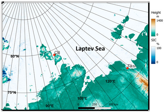
Figure 1.
Model domain of the CCLM model with a 5 km resolution with topography and sea ice concentration for 1 January 2015. The Russian observatories near Tiksi and Cape Baranov (CB) are marked by red dots (topography data from [19]).
In the present paper, a LLJ event in the Tiksi area (31 December 2014 to 1 January 2015) associated with a downslope wind event is studied by observational data and CCLM simulations. The climatology study by [13] on LLJs at Tiksi during the winter of 2014/15, based on SODAR data, showed that LLJs were almost exclusively associated with downslope winds. The case selected in the present study can be regarded as a typical example of the Tiksi area. In contrast to observational studies, the simulations allow for the study of the complete lower troposphere and its spatial structure. The simulations also allow more insight into quantities of the LLJs, which are not directly measured in general, such as the turbulent kinetic energy (TKE).
2. Materials and Methods
2.1. Observations
The observational data for the present study are taken from a field campaign near Tiksi in the Siberian Arctic (Figure 1), which was carried out by the University of Trier and the Arctic and Antarctic Research Institute (AARI, St. Petersburg, Russia) from September 2014 to September 2015. The Tiksi observatory (71.60° N, 128.8°9′ E, 7 m asl) is located about 5 km south of the Tiksi settlement (Yakutia, Russia, see Figure 1 and Figure 2, local time: UTC + 9) at the shoreline of the Buor–Khaya Gulf of the Laptev Sea. The Tiksi observatory (referred to as Tiksi hereafter) is part of a network of long-term Arctic atmospheric observatories [20]. The main topographic feature is the Kharaulaksky Ridge west of the observatory (Figure 2), with elevations up to about 500 m. In addition to the existing instrumentation of the observatory, a SODAR and a RASS (radio acoustic sounding system) owned by the University of Trier were installed during the field campaign at a distance of about 1.6 km northwest of the observatory. The position of the SODAR was close to a meteorological tower, where profiles of wind, temperature, and humidity were measured up to 21 m (Table 1). Data from the SODAR/RASS and the tower were averaged to 1 h means. A detailed description of the instrumentation is given in [13].
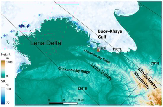
Figure 2.
Map of the Tiksi area with topography and sea ice concentration for 1 January 2015. The position of the Tiksi observatory is marked (topography data from [19]).

Table 1.
Instruments and measurements at the Tiksi observatory used for this study.
2.2. Model Data
Simulations were performed using the non-hydrostatic regional climate model Consortium for Small-Scale Model—Climate Limited Area Mode (CCLM) with a 5 km horizontal resolution. The setup of the model for the Laptev Sea (Figure 1) is the same as in [10]. The model extends vertically up to 22 km with 60 vertical levels; 13 levels are below 500 m in order to obtain a high resolution for the boundary layer. The first model level is 5 m above the surface, and the time resolution of the model output is 1 h. Initial data and boundary data are taken from ERA5 data [21]. The simulations are restarted daily, and no nudging is performed during the simulation time of 30 h. Sea ice concentration (SIC), as shown in Figure 1, is taken as daily data from advanced microwave scanning radiometer 2 (AMSR2) data with 6 km resolution [22]. For the comparison with measurements at Tiksi, the closest model grid point to the SODAR was selected. While the height of the observatory and the tower/SODAR are 7 m and about 20 m asl, respectively, the height of the model grid point is 43 m.
CCLM was evaluated by multiple studies for the Arctic, with one study [10] using near-surface measurements and SODAR measurements at the Russian observatory “Ice Base Cape Baranova” in the Laptev Sea (Figure 1). A comparison of wind profiles from SODAR measurements and CCLM simulations for a three-year period in the area of Severnaya Zemlya (Siberia) showed a positive bias for the wind speed of about 1 m/s below 100 m, which increased to 1.5 m/s for higher levels [10]. Recent verification studies for CCLM using data from the MOSAiC experiment [23] have been performed for near-surface quantities [24] as well as for vertical profiles [25]. The latter study found a wind speed bias of 0.3 m/s in the lower 200 m when comparing CCLM with radiosondes and biases of ±0.1 m/s up to 2000 m.
The representation of the topography in CCLM is shown in Figure 3. Compared with the high-resolution topography shown in Figure 2, the peak heights are smoothed (Figure 3b, see also supplementary Figure S1a). For the study of the LLJ event in Section 3, three cross-sections were selected (Figure 3a). Cross-section A starts over the Buor–Khaya Gulf and goes through the Tiksi grid point (T) approximately in a southwesterly direction. Cross-section B is east of cross-section A and covers a higher part of the Kharaulaksky Ridge. Cross-section C is perpendicular to the Lena Valley.
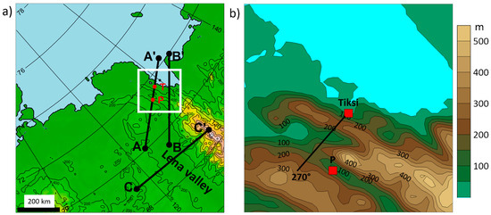
Figure 3.
Map of the Tiksi area with topography of the CCLM model with 5 km horizontal resolution. (a) Locations of cross-sections A, B, and C. T and P mark the locations of Tiksi and an upstream grid point, respectively. (b) Zoomed-in area for the white box indicated in (a). The black line indicates the wind direction of 270°.
3. LLJ Event 31 December 2014 to 1 January 2015
3.1. Observations and Comparison to Simulations
During the period from 31 December 2014 to 1 January 2015, a LLJ event was observed at Tiksi. Figure 4 shows the mean sea level pressure (MSLP), wind speed, and wind direction at 10 m height from the observations and CCLM simulations. This event was one of the LLJ case studies presented in [13]. The measurements of the wind speed at the observatory (resolution 3 h) showed an increase from very weak winds during the first half of 31 December to a maximum of about 7 m/s at 00 UTC on 1 January. Winds around 6 m/s prevailed for the next 12 h, and then the wind dropped below 2 m/s. Data from the tower with 1 h resolution are not available for 31 December, but wind speeds agree with the observatory data on 1 January. The simulations captured the wind increase on 31 December very well, but the decrease on 1 January occurred too early. The wind direction shifted from southwesterly to westerly during the period with increased winds, and the simulations agree better with the tower data. The simulated MSLP is about 1 hPa higher than the observations. In addition to the MSLP at Tiksi, simulated data for the upstream model grid point P (about 65 km southwest of Tiksi, see Figure 3) are shown. During the wind event, the pressure difference between P and Tiksi was positive (about 1.5 hPa), while it dropped to negative values after the event.
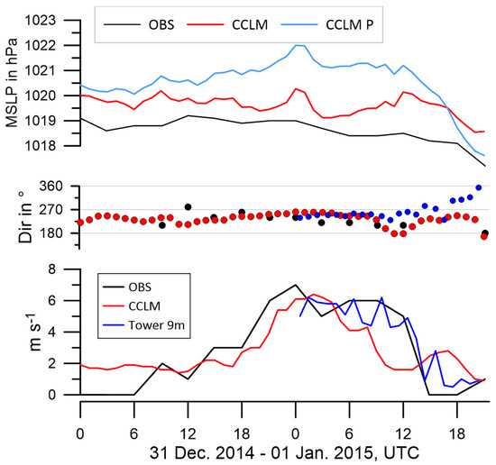
Figure 4.
Mean sea level pressure (MSLP, upper panel), wind direction (middle panel), and wind speed (lower panel) from 31 December 2014 to 1 January 2015 for the measurements at the Tiksi observatory (OBS, black), the tower (blue) and CCLM simulations (red). For MSLP, simulations for point P are also shown (light blue).
Figure 5 shows cross-sections of the lowest 550 m for the wind speed, wind direction, and temperature from simulations and SODAR/RASS data. The simulations (Figure 5a) showed a LLJ at about 200 m height with maximum speeds of about 14 m/s. The simulated wind direction (Figure 5c) showed a westerly flow during the LLJ event and a pronounced change to southerly and southeasterly winds after the LLJ event. The SODAR wind data (Figure 5b,d) generally confirm the simulated structures and evolution. The observed LLJ started at 1200 UTC on 31 December 2014. The observed jet core intensified during the second half of 31 December and rose from 200 m to 300 m. The observed jet speed was slightly weaker than in the simulations. During the first half of 1 January, the observations showed a couple of hours with weaker winds, but then the LLJ intensified again with winds exceeding 10 m/s until 11 UTC on 1 January 2015. For the whole period of the LLJ, the observed wind direction in the jet core was from westerly to northwesterly. Since the range of the RASS was limited to the lowest 250 m, only the thermal structure below the LLJ was captured by the observations. On 1 January 2015, a strong cooling occurred, which can also be seen in the simulations. However, the simulated temperature in the lowest 100 m was too low during the low wind conditions after the LLJ event.
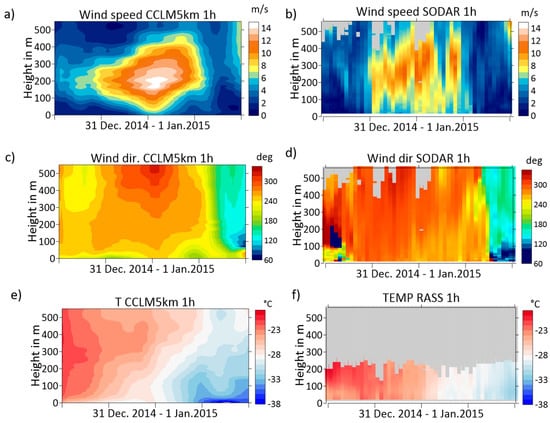
Figure 5.
Time-height cross-sections from 31 December 2014 to 1 January 2015 for the wind speed from simulations (a) and SODAR (b), for the wind direction from simulations (c) and SODAR (d), and the temperature from simulations (e) and RASS (f). Interpolated fields are shown for the simulations, while observations are shown as pixels. Missing data are gray.
3.2. Simulations of the LLJ Evolution and 3D Structure
The simulations allow for the study of the LLJ event for a larger region around the Tiksi observatory. The development of the synoptic environment is shown by the time series of geopotential and wind at 850 and 925 hPa for the Laptev Sea area in Supplementary Figure S2. Prior to the LLJ event at Tiksi, a synoptic cyclone was located about 600 km west of Tiksi, while wind over the northern Laptev Sea was influenced by a strong high-pressure system (Figure S2a,b). At 925 hPa, a belt of stronger winds induced by the topography can be seen around the Kharaulaksky Mountains at 00 UTC on 31 December. The low west of Tiksi remained almost stationary during the next 24 h (Figure S2c,e,g), while the high was replaced by a low moving into the Laptev Sea from the east (Figure S2f,h). The onset of the LLJ event was associated with the southerly flow along the Kharaulaksky Mountains (Figure S2c), while increased pressure gradients associated with the low moving over the Laptev Sea led to increased wind speeds over the Tiksi area (Figure S2e,g).
A more detailed view of the LLJ development is shown in Figure 6 for the wind and pressure at the jet core level (hj) of about 200 m at 12 UTC on 31 December 2014 and 00 UTC on 1 January 2015 for a subdomain of the model (6 hourly plots from 12 UTC on 31 December 2014 to 18 UTC on 1 January 2015 are shown in supplementary Figure S3). At the time of the onset of the LLJ event at Tiksi (Figure 6a), the southerly flow along the Kharaulaksky Mountains through the Lena Valley was also present. This flow can be interpreted as a barrier wind. This air stream passed over the Kharaulaksky Ridge near Tiksi as a southwesterly flow. At 00 UTC on 1 January 2015 (Figure 6b) the barrier wind had decreased, but the southwesterly wind in the Tiksi region was intensified by the increasing synoptic pressure gradient. This situation continued for the next 6 h (Figure S3d), but the pressure gradient and the wind decreased in the Tiksi area by 12 UTC on 1 January Figure S3e), and the wind dropped to very low values afterward (Figure S3f).
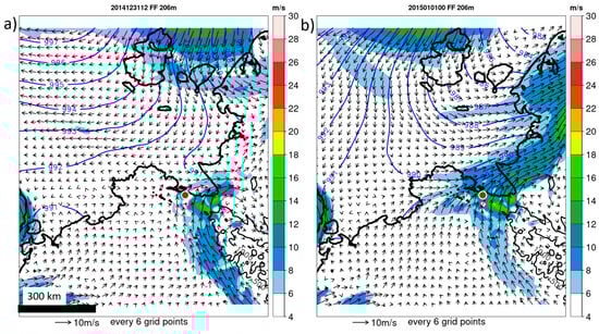
Figure 6.
CCLM simulation of pressure (blue isolines every 1 hPa, only shown over ocean and sea ice), wind speed (shaded), and wind vectors (every 6th grid point) at the LLJ height (206 m) for a subregion of the model domain at (a) 12 UTC on 31 December 2014 and (b) 00 UTC on 1 January 2015. Topography is shown as black isolines every 500 m, and Tiksi is marked by a red dot.
The structure of the barrier flow can be seen in the cross-section C at 12 UTC on 31 December 2014 (Figure 7a). A LLJ with a core speed of about 10 m/s was present at about 200 m above the ground in conditions of stable stratification. While the LLJ was almost completely associated with a wind component normal to the cross-section (parallel to the mountain), the secondary wind maximum west of the jet was associated mainly with westerly flow, which is the typical situation for a barrier wind. This westerly flow weakened during the following 12 h, and the barrier wind decreased (Figure 7b).
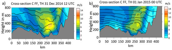
Figure 7.
Cross-section C (view from the south, location see Figure 3) for wind speed (shaded) and potential temperature (isolines every 2 °C) at (a) 12 UTC on 31 December 2014 and (b) 00 UTC on 1 January 2015. Topography is shown in gray.
The wind field at the LLJ height (hj) in the vicinity of Tiksi at 00 UTC on 1 January 2015 is shown in Figure 8a (the distance of wind vectors is 10 km). A band of high wind speeds was located in the lee of the Kharaulaksky Ridge. Two wind maxima were present: one over Tiksi and a second one south of Tiksi over an area of higher elevations. Figure S4 in the supplement shows the temporal development of the wind field as 6 hourly plots from 18 UTC on 31 December 2014 to 18 UTC on 1 January 2015. The wind maximum was associated with a pronounced maximum in wind shear above the jet core (Figure 8b). This wind shear is computed by the difference of the wind speed at twice the jet height V(2hj) and the wind speed at jet height V(hj). The wind decrease above the jet had values of more than 10 m/s above the wind maxima in the lee of the Kharaulaksky Ridge. Since a wind speed anomaly of at least 2 m/s is usually regarded as a LLJ (see, e.g., [2,4]), the topographic LLJ extended over a distance of more than 100 km along the mountains but also about 50 km downstream. Tiksi was located below a local wind maximum for the whole period, but only at 18 UTC on 31 December 2014, and it was also in the region of maximum vertical wind shear (Figure S4b). The vertical wind shear (and thus the LLJ) was most pronounced for the mountain slope south of Tiksi at 06 UTC on 1 January 2015 (Figure S4f). Wind maxima and vertical wind shear weakened during the next 6 h (Figure S4g,h) and disappeared at 18 UTC on 1 January 2015 (Figure S4i,j).
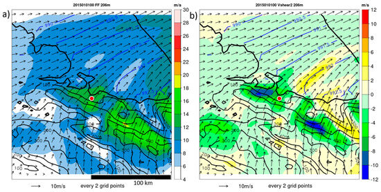
Figure 8.
CCLM simulation of pressure (isolines every 0.5 hPa, only shown over ocean and sea ice) and wind vectors (every 2nd grid point) at the LLJ height (206 m) for a subregion of the model domain at 00 UTC on 1 January 2015 with (a) wind speed and (b) wind shear above the jet (V(2hj)—V(hj)). Topography is shown as black isolines every 100 m, and Tiksi is marked by a red dot.
The structure of the flow affecting Tiski is now studied in cross-section A, which is approximately oriented in the flow direction at the jet level near Tiksi (Figure 9). At 12 UTC on 31 December 2014 (Figure 9a), a LLJ with a core speed of about 8 m/s was present above Tiksi. The LLJ was associated with a lee wave and a stable stratification of the flow. The temperature in the lowest 400 m was about 2–3 °C higher downstream of Tiksi compared with the flow upstream of the mountain ridge. At 00 UTC on 1 January 2015 (Figure 9b), the LLJ and the lee wave had intensified, and a cooling of about 4 °C occurred throughout the cross-section. At that time, the increased pressure gradient associated with the low moving over the Laptev Sea (Figure 6b) caused the advection of cold air toward Tiksi. Six hours later (Figure 9c), further cooling and stabilization of the upstream flow had taken place. More lee waves can be seen upstream, e.g., also for the Chekanovsky Ridge (see Figure 2). The LLJ at Tiksi had split into two wind maxima, and the potential temperature structure associated with the maximum downstream of Tiksi resembled a hydraulic jump. The lee wave at Tiksi was most pronounced at that time, and signatures of wave breaking were present. At 12 UTC on 1 January 2015 (Figure 9d), the wind had decreased since the synoptic pressure gradient weakened (Figure S4f).
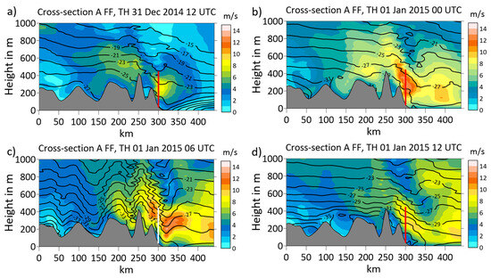
Figure 9.
Cross-section A (view from the southeast, location see Figure 3) for wind speed (shaded) and potential temperature (isolines every 2 °C) at (a) 12 UTC on 31 December 2014, (b) 00 UTC on 1 January 2015, (c) 06 UTC on 1 January 2015 and (d) 12 UTC on 1 January 2015. Topography is shown in gray, and the vertical line (red or white) marks the position of Tiksi and the range of the SODAR.
The structure and evolution of the LLJ over the mountain slope south of Tiksi is shown in cross-section B, which is again approximately orientated in the flow direction at the jet level in that area (Figure 10). The mountain ridge is less structured compared with cross-section A, and the peak height is about 100 m higher. At 12 UTC on 31 December 2014 (Figure 10a), the mountain wave and the LLJ were already well-developed. The lowest 300 m were only weakly stable, creating favorable conditions for the flow over the mountain. As discussed for cross-section A, a general cooling occurred in the next 12 h (Figure 10b), followed by a stabilization of the lowest 300 m in the upstream flow (Figure 10c). The LLJ and the lee wave remained almost unchanged until 06 UTC on 1 January 2015. The temperature in the lowest 400 m was about 2–3 °C higher downstream compared with the flow upstream of the mountain ridge. At 12 UTC on 1 January 2015 (Figure 10d), the upstream flow and the LLJ had weakened in accordance with the decreasing synoptic pressure gradient (Figure S4f).
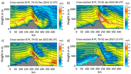
Figure 10.
Cross-section B (view from the southeast, location see Figure 3) for wind speed (shaded) and potential temperature (isolines every 2 °C) at (a) 12 UTC on 31 December 2014, (b) 00 UTC on 1 January 2015, (c) 06 UTC on 1 January 2015 and (d) 12 UTC on 1 January 2015. Topography is shown in gray.
4. Discussion
The LLJ event occurring from 31 December 2014 to 1 January 2015 at Tiksi was studied by synoptic observations and SODAR/RASS data by [13]. They found that the LLJ developed during conditions of only high or mid-level clouds and that a near-surface cooling of about 10 K occurred during the LLJ event.
The CCLM simulations reproduce the near-surface and SODAR/RASS observations during the LLJ event relatively well (Figure 4 and Figure 5). While the observed jet core rose from 200 m to 300 m during its development, it stayed at the same height in the simulations. The observed jet speed was slightly weaker than in the simulations. This event was classified by [13] as a strong jet (exceeding 10 m/s). They found no signs of an inertial oscillation, but mainly the increase and decrease of the westerly wind for the intensification and decay of the jet. Since their climatology for LLJs for the winter 2014/15 showed that LLJs were almost exclusively associated with westerly winds at the jet level, the case selected in the present study can be regarded as a typical example for the Tiksi area.
The present study shows the relationship between the LLJ event and a downslope wind event associated with a pronounced lee wave, enabling a detailed analysis of the synoptic environment and processes leading to the LLJ evolution. Not only the local topography, but also the large-scale environment provided by the Kharaulaksky Mountains were relevant for the LLJ development. The flow was preconditioned by a barrier wind and channeling in the Lena Valley (also associated with a LLJ) in the initial phase, but the synoptic forcing by a low over the Laptev Sea was dominant in the mature and dissipation phase of the LLJ. Throughout the event, a positive MSLP difference of about 1.5 hPa was present between an upstream grid point and Tiksi (Figure 4), which was in accordance with the mountain wave formation at the Kharaulaksky Ridge, which caused the downslope wind event.
The area around Tiksi was identified as one of the main regions for downslope wind storms in the Russian Arctic by [16]. A study using high-resolution (1 km) simulations for a downslope wind event occurring from 26 to 27 December 1980 at Tiksi [8] showed that the standard setup of the WRF model led to a large underestimation of the simulated near-surface wind speed and that the structure and position of the wind maximum depends on the parameterization of the surface roughness. The CCLM simulations showed good agreement with the near-surface wind and the LLJ, but also that the LLJ varied in position during its evolution. This is demonstrated in Figure 11, which shows a subsection of cross-section A (see Figure 9) at 00 and 06 UTC on 1 January 2015. In contrast to Figure 9, the horizontal wind component along the cross-section (Uc) is shown. The similarity to Figure 9 shows that Uc dominates the wind speed; that is, the wind component along the mountain ridge is small. The wind vectors showed the development of the lee wave and its relationship with the LLJ. The split of the LLJ core between 00 and 06 UTC was associated with the formation of a second wave structure downwind of Tiksi. As already mentioned in the last Section, this structure resembled a hydraulic jump, and signatures of wave breaking were present at higher levels. This is associated with relatively high values of TKE, which had maximum values of more than 0.7 m2/s2 at 06 UTC. Other regions with high TKE were found below the LLJs over the slope and downstream of Tiksi, respectively. This underlines the impact of LLJs on turbulent processes in the ABL, which was also found in previous studies of LLJs [2,26,27]. The relationship between wave breaking and high TKE values was shown by [28] in a case study of a severe downslope windstorm in Iceland. While the mountain was much higher (about 2000 m) and the wind speed was much larger (more than 40 m/s), the TKE structure resembles the structure found for the Tiksi area in the present study. A case study for mountain heights comparable to the Tiksi area [29] showed that a downslope windstorm with near-surface winds up to about 20 m/s was produced under favorable conditions of wind and temperature profiles, even for modest topography.
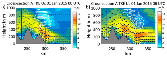
Figure 11.
Subsection of cross-section A (view from the southeast, location see Figure 3) for the horizontal wind component along the cross-section (shaded), wind vectors (every 2nd grid point and level, vertical wind with a factor of 100) and TKE (isolines for 0.1, 0.4 and 0.7 m²/s², cross-hatched for >0.4 m²/s²) at (a) 00 UTC on 1 January 2015 and (b) 06 UTC on 1 January 2015. Topography is shown in gray, and the vertical red line marks the position of Tiksi and the range of the SODAR, while the vertical blue line marks the position of point P.
Recent global climatologic studies of downslope winds [30] and LLJs [1] based on ERA5 data indicate that increased frequencies of both phenomena are present along the Kharaulaksky Mountains. This is in agreement with the climatology of LLJs based on ASR data with 30 km resolution by [15], who showed a LLJ frequency of 60–70% in the region of the Kharaulaksky Mountains during winter. However, the coarse resolution of ERA5 or ASR is not suitable for studies of mountain wave processes in the Tiksi area. The ERA5 topography shown in Figure S1b does neither resolve the Kharaulaksky Ridge nor the Lena Valley. In contrast, the CCLM topography (Figure 3) resolves the main topographic features reasonably well compared with Figure S1a, but subgrid-scale topographic structures may also affect the flow conditions at the site of the Tiksi observatory [13].
The present study contributes to the understanding of the formation of LLJs in the Siberian Arctic, which is relevant, e.g., for aircraft operations, air pollution, and wind energy [31]. In the Tiksi region, strong downslope windstorms were found to be associated with turbulence that poses a hazard for light aircraft [18]. Ongoing work comprises a detailed evaluation of CCLM using the SODAR observations at Tiksi for one year (2014/15). Future work will include climatological studies of LLJs in the Tiksi area using CCLM simulations with 5 km resolution for the period 2014–2020.
5. Summary and Conclusions
Simulations were performed using the regional climate model CCLM with a 5 km resolution with nesting in ERA5 data for a LLJ event occurring from 31 December 2014 to 1 January 2015, and ABL measurements were used for comparison. The main conclusions are as follows:
- −
- CCLM simulations agree well with near-surface and SODAR/RASS observations.
- −
- The LLJ at Tiksi was part of a downslope wind event, and LLJ structures were present for a large region.
- −
- The flow was preconditioned by a barrier wind and channeling in the Lena Valley (also associated with a LLJ) during the initial phase, but synoptic forcing by a low over the Laptev Sea was dominant in the mature and dissipation phases of the LLJ.
- −
- Wave breaking with high TKE values seemed to occur in the mature phase of the LLJ.
- −
- Downslope wind events are likely the reason for most LLJs at Tiksi.
Supplementary Materials
The following supporting information can be downloaded at https://www.mdpi.com/article/10.3390/meteorology4010007/s1, Figure S1. Map of the Tiksi area with topography for 1 km horizontal resolution and ERA5 data. Figure S2. CCLM simulation of geopotential and wind at 925 and 850 hPa for the Laptev Sea from 00 UTC on 31 December to 12 UTC on 1 January 2015. Figure S3. CCLM simulation of pressure and wind at the LLJ height (206 m) for a subregion of the model domain from 12 UTC on 31 December 2014 to 18 UTC on 1 January 2015. Figure S4. CCLM simulation of pressure, wind at the LLJ height (206 m), and wind shear above the jet for a subregion of the model domain from 18 UTC on 31 December 2014 to 18 UTC on 1 January 2015.
Funding
This research was funded by the Federal Ministry of Education and Research (BMBF) under grant 03F0831C in the frame of German-Russian cooperation “WTZ RUS: Changing Arctic Transpolar System (CATS)”.
Institutional Review Board Statement
Not applicable.
Informed Consent Statement
Not applicable.
Data Availability Statement
SODAR/RASS data are publicly available on PANGAEA [32]. Data from the Tiski observatory and the Tiksi tower were obtained from NOAA via ftp://ftp.ncdc.noaa.gov/pub/data/gsod. Model data are available on a permanent data archive at the Deutsches Klimarechenzentrum (DKRZ) via https://hdl.handle.net/21.14106/d6370870d522874d91d18f1f5282baec67e02ce3 (accessed on 7 March 2025). ERA5 data are provided for the CCLM community (www.clm-community.eu) via the DKRZ data pool and by the Copernicus Climate Change Service (C3S) Climate Data Store (CDS) [33].
Acknowledgments
Thanks to the CLM Community and the German Meteorological Service for providing the basic CCLM model. This work used resources of the Deutsches Klimarechenzentrum (DKRZ) granted by its Scientific Steering Committee (WLA) under project ID bb0474. Thanks to colleagues at GEOMAR Kiel and AARI for logistic support in the framework of the interdisciplinary CATS project, to Pascal Schwarz and Clemens Drüe for performing and processing SODAR/RASS data, to Lukas Schefczyk for performing the CCLM simulations and Rolf Zentek for help with processing CCLM data. Model data processing was performed using Climate Data Operators (CDO) (https://doi.org/10.5281/zenodo.3539275) and R software (version 4.4.0).
Conflicts of Interest
The author declares no conflicts of interest.
References
- Luiz, E.W.; Fiedler, S. Global Climatology of Low-Level-Jets: Occurrence, Characteristics, and Meteorological Drivers. J. Geophys. Res. Atmos. 2024, 129, e2023JD040262. [Google Scholar] [CrossRef]
- Heinemann, G.; Schefczyk, L.; Zentek, R. A model-based study of the dynamics of Arctic low-level jet events for the MOSAiC drift. Elem. Sci. Anthr. 2024, 12, 00064. [Google Scholar] [CrossRef]
- Jakobson, L.; Vihma, T.; Jakobson, E.; Palo, T.; Männik, A.; Jaagus, J. Low-level jet characteristics over the Arctic Ocean in spring and summer. Atmos. Meas. Tech. 2013, 13, 11089–11099. [Google Scholar] [CrossRef]
- López-García, V.; Neely, R.R.; Dahlke, S.; Brooks, I.M. Low-level jets over the Arctic Ocean during MOSAiC. Elem. Sci. Anthr. 2022, 10, 00063. [Google Scholar] [CrossRef]
- Guest, P.; Persson, P.O.G.; Wang, S.; Jordan, M.; Jin, Y.; Blomquist, B.; Fairall, C. Low-Level Baroclinic Jets Over the New Arctic Ocean. J. Geophys. Res. Oceans 2018, 123, 4074–4091. [Google Scholar] [CrossRef]
- Andreas, E.L.; Claffy, K.J.; Makshtas, A.P. Low-Level Atmospheric Jets and Inversions Over the Western Weddell Sea. Bound. Layer Meteorol. 2000, 97, 459–486. [Google Scholar] [CrossRef]
- Heinemann, G. The KABEG’97 field experiment: An aircraft-based study of katabatic wind dynamics over the Greenland ice sheet. Bound. Layer Meteorol. 1999, 93, 75–116. [Google Scholar] [CrossRef]
- Shestakova, A.A. Impact of land surface roughness on downslope windstorm modelling in the Arctic. Dyn. Atmos. Oceans 2021, 95, 101244. [Google Scholar] [CrossRef]
- Samelson, R.M.; Barbour, P.L. Low-Level Jets, Orographic Effects, and Extreme Events in Nares Strait: A Model-Based Mesoscale Climatology. Mon. Weather Rev. 2008, 136, 4746–4759. [Google Scholar] [CrossRef]
- Heinemann, G.; Drüe, C.; Makshtas, A. A Three-Year Climatology of the Wind Field Structure at Cape Baranova (Severnaya Zemlya, Siberia) from SODAR Observations and High-Resolution Regional Climate Model Simulations during YOPP. Atmosphere 2022, 13, 957. [Google Scholar] [CrossRef]
- Kohnemann, S.H.; Heinemann, G. A climatology of wintertime low-level jets in Nares Strait. Polar Res. 2021, 40, 3622. [Google Scholar] [CrossRef]
- Heinemann, G. An Aircraft-Based Study of Strong Gap Flows in Nares Strait, Greenland. Mon. Weather Rev. 2018, 146, 3589–3604. [Google Scholar] [CrossRef]
- Heinemann, G.; Drüe, C.; Schwarz, P.; Makshtas, A. Observations of Wintertime Low-Level Jets in the Coastal Region of the Laptev Sea in the Siberian Arctic Using SODAR/RASS. Remote Sens. 2021, 13, 1421. [Google Scholar] [CrossRef]
- Bromwich, D.H.; Wilson, A.B.; Bai, L.; Moore, G.W.K.; Bauer, P. A comparison of the regional Arctic System Reanalysis and the global ERA-Interim Reanalysis for the Arctic. Q. J. R. Meteorol. Soc. 2016, 142, 644–658. [Google Scholar] [CrossRef]
- Tuononen, M.; Sinclair, V.A.; Vihma, T. A climatology of low-level jets in the mid-latitudes and polar regions of the Northern Hemisphere. Atmos. Sci. Lett. 2015, 16, 492–499. [Google Scholar] [CrossRef]
- Shestakova, A.A.; Toropov, P.A.; Matveeva, T.A. Climatology of extreme downslope windstorms in the Russian Arctic. Weather Clim. Extrem. 2020, 28, 100256. [Google Scholar] [CrossRef]
- Bromwich, D.H.; Wilson, A.B.; Bai, L.; Liu, Z.; Barlage, M.; Shih, C.-F.; Maldonado, S.; Hines, K.M.; Wang, S.-H.; Woollen, J.; et al. The Arctic System Reanalysis, Version 2. Bull. Am. Meteorol. Soc. 2018, 99, 805–828. [Google Scholar] [CrossRef]
- Shestakova, A.A. Assessing the Risks of Vessel Icing and Aviation Hazards during Downslope Windstorms in the Russian Arctic. Atmosphere 2021, 12, 760. [Google Scholar] [CrossRef]
- GMTED. Global Multi-Resolution Terrain Elevation Data 2010 (GMTED2010). Available online: https://cmr.earthdata.nasa.gov:443/search/concepts/C1220567856-USGS_LTA.html (accessed on 3 September 2024).
- Uttal, T.; Starkweather, S.; Drummond, J.R.; Vihma, T.; Makshtas, A.P.; Darby, L.S.; Burkhart, J.F.; Cox, C.J.; Schmeisser, L.N.; Haiden, T.; et al. International Arctic Systems for Observing the Atmosphere: An International Polar Year Legacy Consortium. Bull. Am. Meteorol. Soc. 2016, 97, 1033–1056. [Google Scholar] [CrossRef]
- Hersbach, H.; Bell, B.; Berrisford, P.; Hirahara, S.; Horányi, A.; Muñoz-Sabater, J.; Nicolas, J.; Peubey, C.; Radu, R.; Schepers, D.; et al. The ERA5 global reanalysis. Q. J. R. Meteorol. Soc. 2020, 146, 1999–2049. [Google Scholar] [CrossRef]
- Spreen, G.; Kaleschke, L.; Heygster, G. Sea ice remote sensing using AMSR-E 89-GHz channels. J. Geophys. Res. Oceans 2008, 113, C02S03. [Google Scholar] [CrossRef]
- Shupe, M.D.; Rex, M.; Blomquist, B.; Persson, P.O.G.; Schmale, J.; Uttal, T.; Althausen, D.; Angot, H.; Archer, S.; Bariteau, L.; et al. Overview of the MOSAiC expedition: Atmosphere. Elem. Sci. Anthr. 2022, 10, 00060. [Google Scholar] [CrossRef]
- Heinemann, G.; Schefczyk, L.; Willmes, S.; Shupe, M.D. Evaluation of simulations of near-surface variables using the regional climate model CCLM for the MOSAiC winter period. Elem. Sci. Anthr. 2022, 10, 00033. [Google Scholar] [CrossRef]
- Heinemann, G.; Schefczyk, L.; Zentek, R.; Brooks, I.M.; Dahlke, S.; Walbröl, A. Evaluation of Vertical Profiles and Atmospheric Boundary Layer Structure Using the Regional Climate Model CCLM during MOSAiC. Meteorology 2023, 2, 257–275. [Google Scholar] [CrossRef]
- Duarte, H.F.; Leclerc, M.Y.; Zhang, G.; Durden, D.; Kurzeja, R.; Parker, M.; Werth, D. Impact of Nocturnal Low-Level Jets on Near-Surface Turbulence Kinetic Energy. Bound. Layer Meteorol. 2015, 156, 349–370. [Google Scholar] [CrossRef]
- Heinemann, G. Aircraft-Based Measurements of Turbulence Structures in the Katabatic Flow Over Greenland. Bound. Layer Meteorol. 2002, 103, 49–81. [Google Scholar] [CrossRef]
- Ólafsson, H.; Ágústsson, H. The Freysnes downslope windstorm. Meteorol. Z. 2007, 16, 123–130. [Google Scholar] [CrossRef]
- Decker, S.G.; Robinson, D.A. Unexpected High Winds in Northern New Jersey: A Downslope Windstorm in Modest Topography. Weather Forecast. 2011, 26, 902–921. [Google Scholar] [CrossRef]
- Abatzoglou, J.T.; Hatchett, B.J.; Fox-Hughes, P.; Gershunov, A.; Nauslar, N.J. Global climatology of synoptically-forced downslope winds. Int. J. Clim. 2021, 41, 31–50. [Google Scholar] [CrossRef]
- Ivanova, I.Y.; Nogovitsyn, D.D.; Tuguzova, T.F.; Shakirov, V.A.; Sheina, Z.M.; Sergeeva, L.P. The use of wind potential in the local energy of Yakutia. IOP Conf. Ser. Mater. Sci. Eng. 2020, 905, 12050. [Google Scholar] [CrossRef]
- Heinemann, G.; Drüe, C. SODAR/RASS Profiles and Low-Level Jets at Tiksi Observatory in 2014/2015, Laptev Sea; PANGAEA: Bremen, Germany, 2021. [Google Scholar] [CrossRef]
- Copernicus Climate Change Service. ERA5 Hourly Data on Single Levels from 1940 to Present, Copernicus Climate Change Service (C3S) Climate Data Store (CDS). 2023. Available online: https://cds.climate.copernicus.eu/datasets/reanalysis-era5-single-levels?tab=overview (accessed on 7 March 2024).
Disclaimer/Publisher’s Note: The statements, opinions and data contained in all publications are solely those of the individual author(s) and contributor(s) and not of MDPI and/or the editor(s). MDPI and/or the editor(s) disclaim responsibility for any injury to people or property resulting from any ideas, methods, instructions or products referred to in the content. |
© 2025 by the author. Licensee MDPI, Basel, Switzerland. This article is an open access article distributed under the terms and conditions of the Creative Commons Attribution (CC BY) license (https://creativecommons.org/licenses/by/4.0/).