

Machine Learning with Voting Committee for Frost Prediction

 , , and
Abstract
1. Introduction
2. Materials and Methods
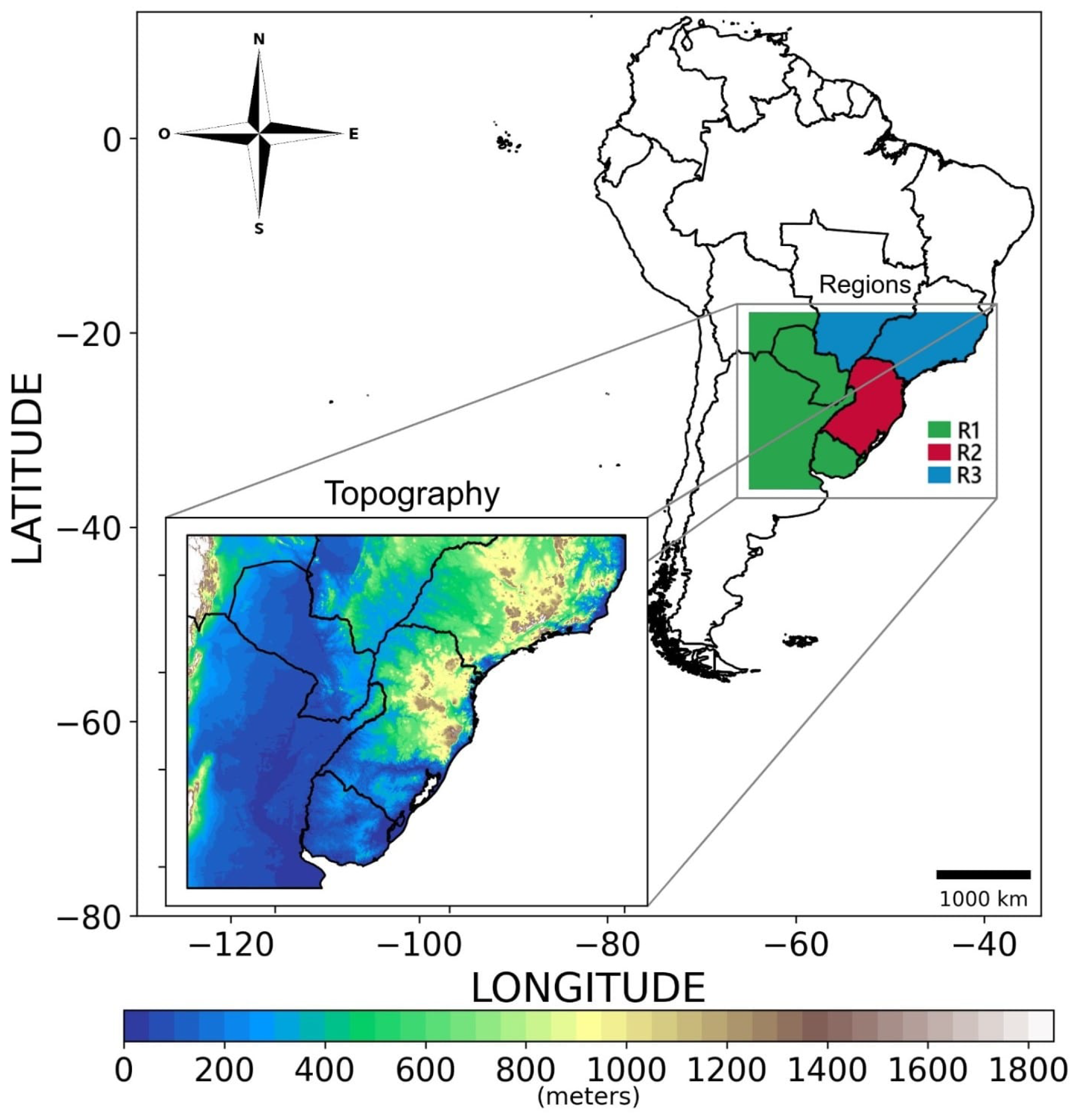
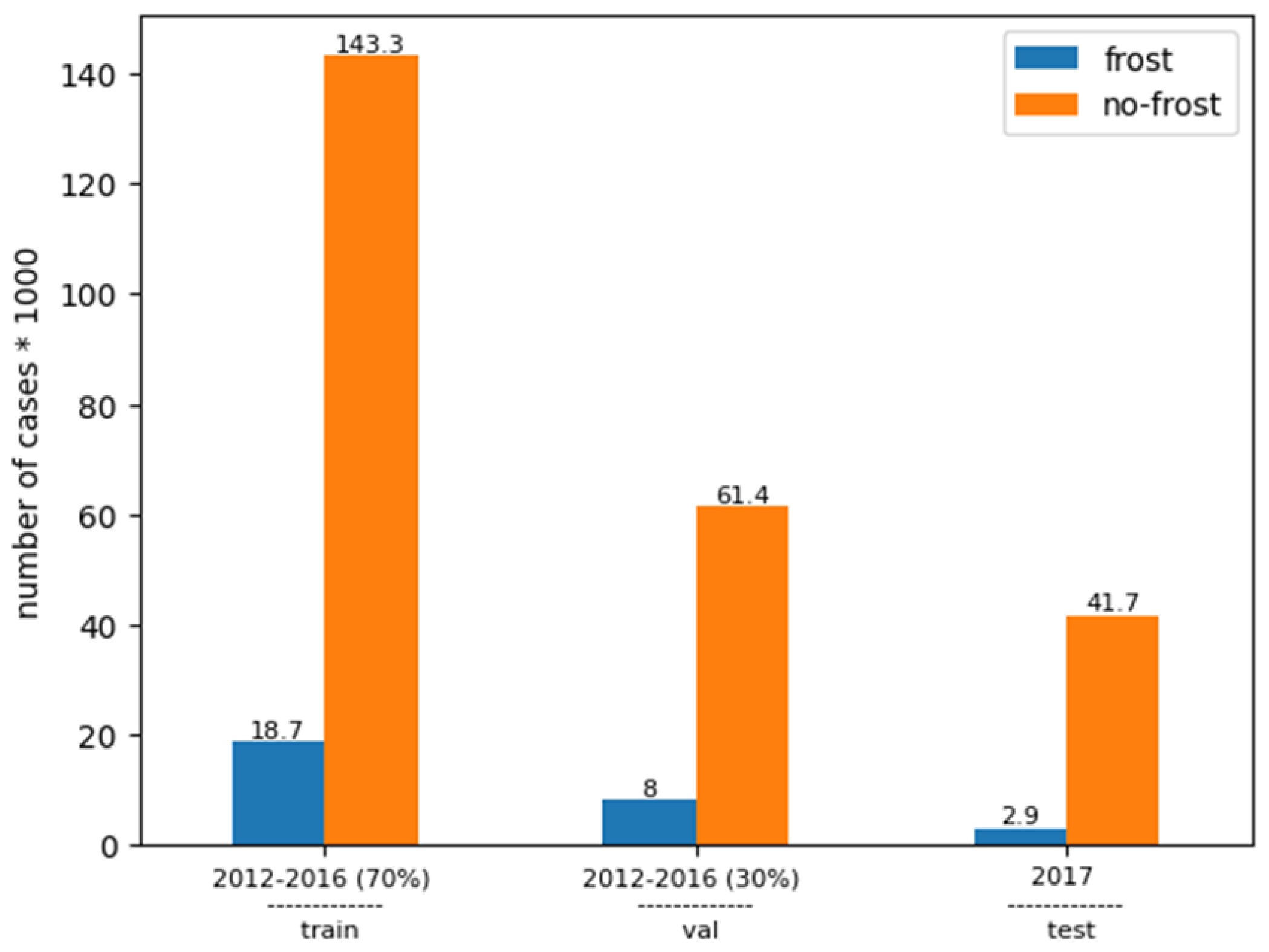
2.1. Data
2.2. IG-Frost Index
2.3. Neural Network
2.4. Voting Committee
2.5. Evaluation Metrics
2.6. Description of Experiments
3. Results
3.1. 24 h Forecast
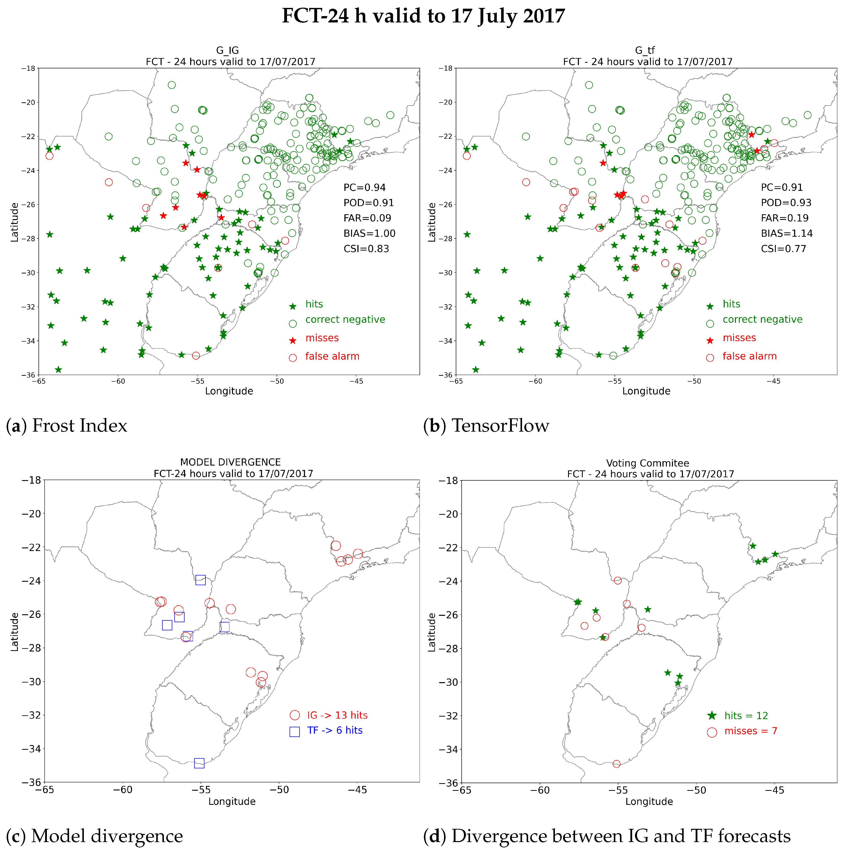
3.1.1. Frost Predictions: 17 July 2017
3.1.2. Frost Predictions: 18 July 2017
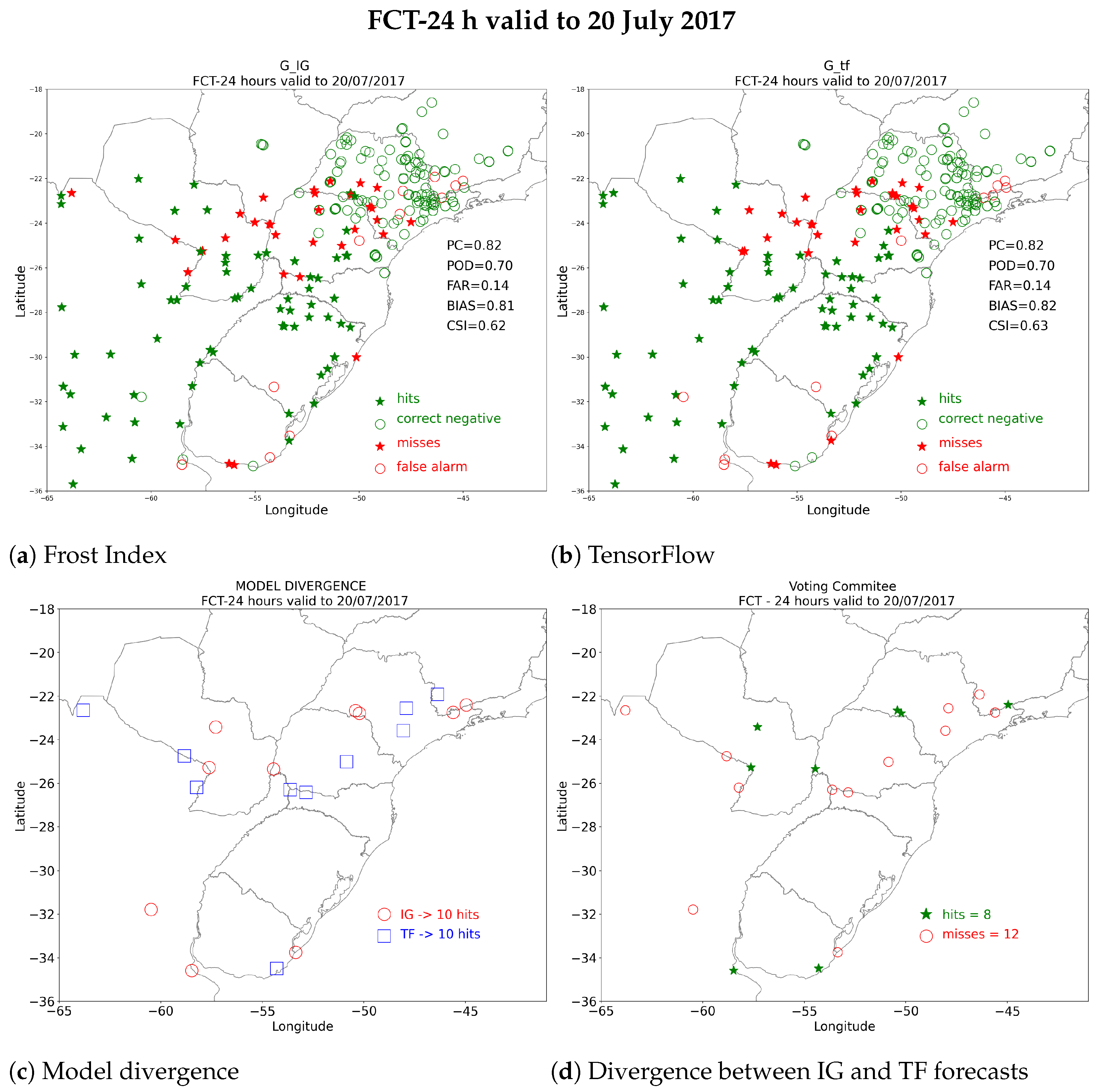
3.1.3. Frost Predictions: 20 July 2017
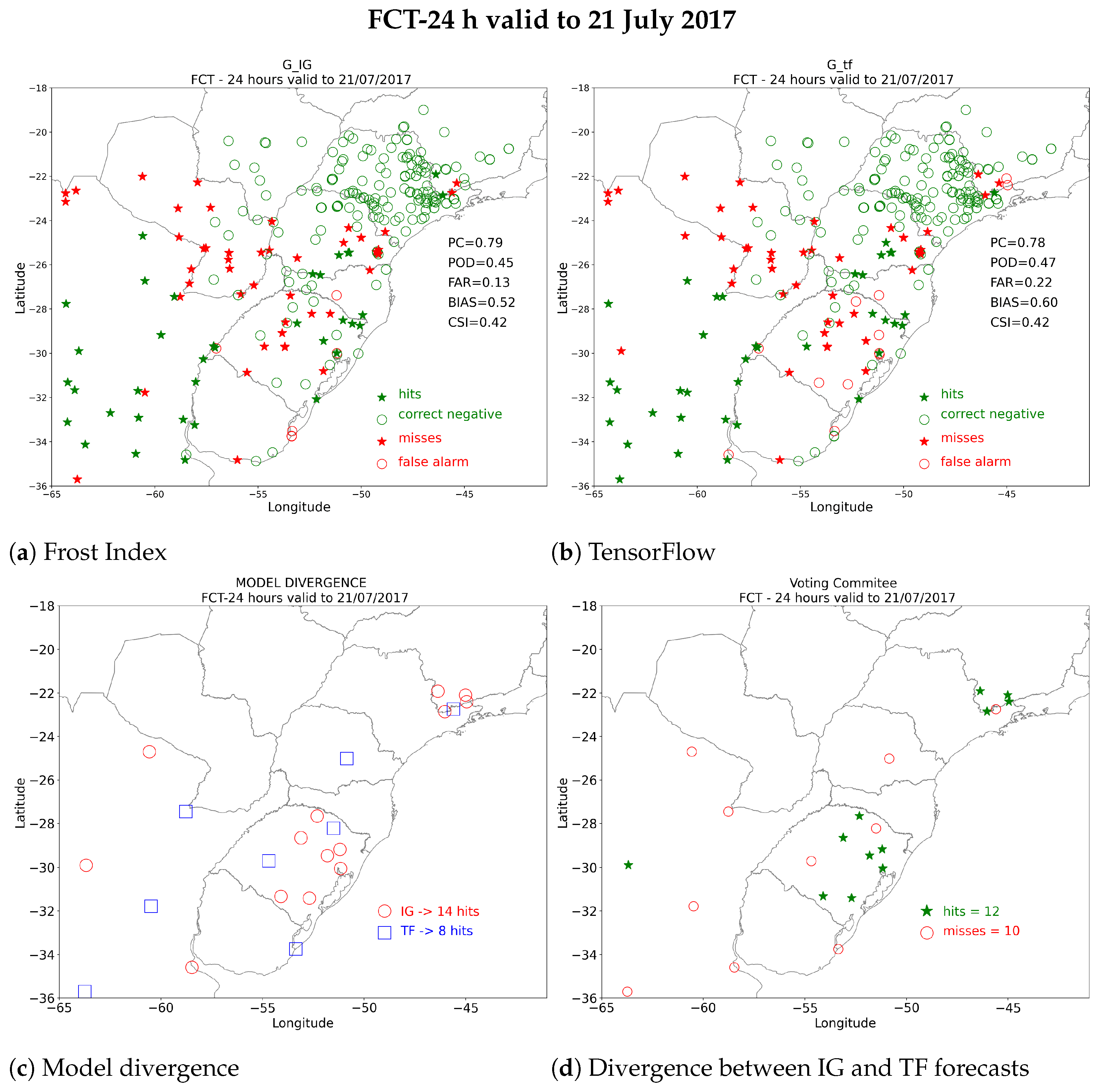
3.1.4. Frost Predictions: 21 July 2017
3.1.5. Frost Predictions: 24 July 2017
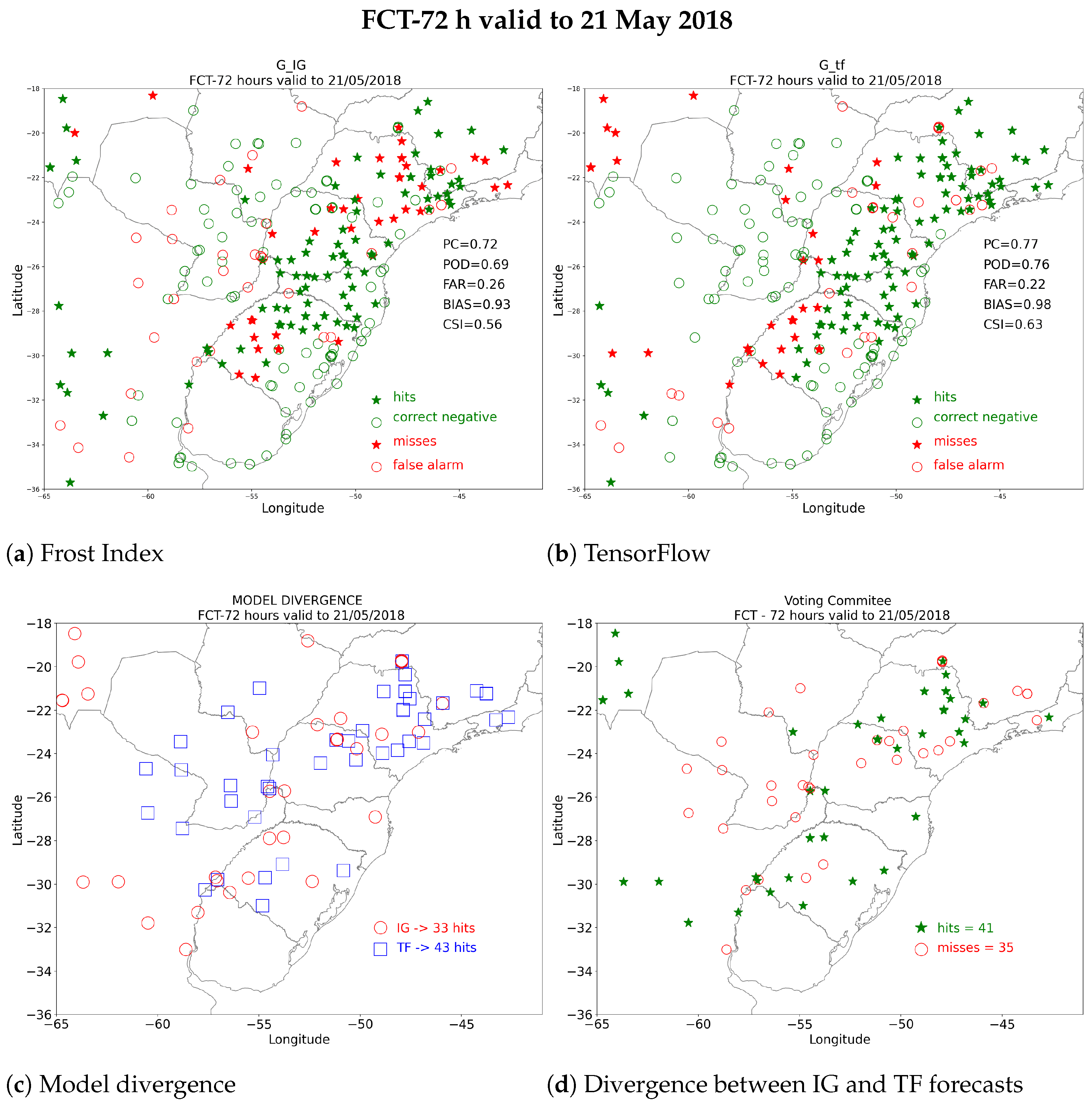
3.2. 72 h Forecast
4. Discussion and Conclusions
Author Contributions
Funding
Institutional Review Board Statement
Informed Consent Statement
Data Availability Statement
Acknowledgments
Conflicts of Interest
References
- Margolis, M.L. Green gold and ice: The impact of frost on the coffee growing region of Northern Paraná, Brazil. Mass Emergencies 1979, 4, 135–144. [Google Scholar]
- Hewitt, K. Interpreting the role of hazards in agriculture. In Interpretations of Calamity; Hewitt, K., Ed.; Allen Unwin: London, UK, 1983; pp. 123–139. [Google Scholar]
- Moricochi, L.; Alfonsi, R.R.; Oliveira, E.D.; de Monteiro, J.L.M. Geadas e seca de 1994: Perspectivas do mercado cafeeiro. Informações Econômicas 1995, 25, 49–57. [Google Scholar]
- Junges, A.; Fontana, D. Quebras de safra de trigo no estado do Rio Grande do Sul: Um estudo de caso. In Proceedings of the XVI Congresso Brasileiro de Agrometeorologia, Belo Horizonte, Brazil, 22–25 September 2009. [Google Scholar]
- Melo, C.; Moro, L. Sazonalidade de Preços do Trigo no Paraná de 2000 a 2012. Revista de Política Agrícola, Local de Publicação (Editar no Plugin de Tradução o Arquivo da Citação ABNT). 22 June 2015. Available online: https://seer.sede.embrapa.br/index.php/RPA/article/view/852 (accessed on 15 December 2020).
- Tsunechiro, A.; Miura, M. Segunda Estimativa de Oferta e Demanda de Milho no estado de São Paulo em 2009; Informações Econômicas: São Paulo, Brazil, 2009; Volume 39. [Google Scholar]
- Blanc, M.L.; Geslin, H.; Holzberg, I.; Mason, B. Protection Against Frost Damage; WMO: Genova, Italy, 1963. [Google Scholar]
- Bettencourt, M.L. Contribuição para o Estudo das Geadas em Portugal Continental; Instituto Nacional de Meteorologia e Geofísica: Lisboa, Portugal, 1980.
- Mota, F.S. Balanço hídrico. In Meteorologia Agrícola; Nobel: São Paulo, Brazil, 1987; pp. 279–309. [Google Scholar]
- Cunha, F.R. O Problema da Geada Negra no Algarve; Series Divulgação. 12; INIA: Instituto Nacional de Investigacao Agraria: Lisbon, Portugal, 1982; 125p. (In Portuguese)
- Hogg, W.H. Frequency of radiation and wind frosts during spring in Kent. Meteorol. Mag. 1950, 79, 42–49. [Google Scholar]
- Hogg, W.H. Spring frosts. Agriculture 1971, 78, 28–31. [Google Scholar]
- Lawrence, E.N. Frost investigation. Meteorol. Mag. 1952, 81, 65–74. [Google Scholar]
- Raposo, J.R. A Defesa das Plantas Contra as Geadas. Junta de Colonização Interna, Estudos Técnicos. 1967; Volume 7, p. 111. (In Portuguese). Available online: https://livrariadalapa.com/categorias/2144-jose-rasquilho-raposo-a-defesa-das-plantas-contra-as-geadas (accessed on 7 October 2024).
- Hewett, E.W. Preventing Frost Damage to Fruit Trees; New Zealand Department of Scientific and Industrial Research (DSIR) Information Series, No. 86; 1971; 55p. Available online: https://books.google.com.br/books?id=8eRL0AEACAAJ (accessed on 7 October 2024).
- Cunha, J.M. Contribuição para o Estudo do Problema das Geadas em Portugal; 1952 Relatório Final do Curso de Engenheiro Agrónomo; Instituto Superior de Agronomia: Lisbon, Portugal, 1952. (In Portuguese) [Google Scholar]
- Snyder, R.L.; de Melo-Abreu, J.P. Frost Protection: Fundamentals, Practice and Economics; Environmental and Natural Resouces Series; FAO: Rome, Italy, 2005; Volume 1. [Google Scholar]
- Diedrichs, A.L.; Bromberg, F.; Dujovne, D.; Brun-Laguna, K.; Watteyne, T. Prediction of frost events using machine learning and IoT sensing devices. IEEE Internet Things J. 2018, 5, 4589–4597. [Google Scholar] [CrossRef]
- Ding, L.; Noborio, K.; Shibuya, K. Frost forecast using machine learning-from association to causality. Procedia Comput. Sci. 2019, 159, 1001–1010. [Google Scholar] [CrossRef]
- Fuentes, M.; Cristóbal, C.; García-Loyola, S. Application of artificial neural networks to frost detection in central Chile using the next day minimum air temperature forecast. Chil. J. Agric. Res. 2018, 78, 327–338. [Google Scholar] [CrossRef]
- Maqsood, I.; Khan, M.R.; Abraham, A. An ensemble of neural networks for weather forecasting. Neural Comput. Appl. 2004, 13, 112–122. [Google Scholar] [CrossRef]
- Lira, H.; Martí, L.; Sanchez-Pi, N. A graph neural network with spatio-temporal attention for multi-sources time series data: An application to frost forecast. Sensors 2022, 22, 1486. [Google Scholar] [CrossRef]
- Talsma, C.J.; Solander, K.C.; Mudunuru, M.K.; Crawford, B.; Powell, M.R. Frost prediction using machine learning and deep neural network models. Front. Artif. Intell. 2023, 5, 963781. [Google Scholar] [CrossRef] [PubMed]
- Wassan, S.; Xi, C.; Jhanjhi, N.Z.; Binte-Imran, L. Effect of frost on plants, leaves, and forecast of frost events using convolutional neural networks. Int. J. Distrib. Sens. Netw. 2021, 17, 15501477211053777. [Google Scholar] [CrossRef]
- Rozante, J.R.; Gutierrez, E.R.; da Silva Dias, P.L.; de Almeida Fernandes, A.; Alvim, D.S.; Silva, V.M. Development of an index for frost prediction: Technique and validation. Meteorol. Appl. 2020, 27, e1807. [Google Scholar] [CrossRef]
- Rozante, J.R.; Ramirez, E.; Ramirez, D.; Rozante, G. Improved frost forecast using machine learning methods. Artif. Intell. Geosci. 2023, 4, 164–181. [Google Scholar] [CrossRef]
- Haykin, S. Neural Networks: A Comprehensive Foundation, 2nd ed.; Prentice Hall, Inc.: Hoboken, NJ, USA, 1999. [Google Scholar]
- Pinto, H.C.; Tarifa, J.R.; Alfonsi, R.R.; Pedro, M.J.J. Estimation of Frost Damage in Coffee Trees in the State of São Paulo, Brazil; American Meteorological Society: Boston, MA, USA, 1977; pp. 37–38. [Google Scholar]
- Black, T.L. The new NMC mesoscale Eta model: Description and forecast examples. Weather. Forecast. 1994, 9, 265–278. [Google Scholar] [CrossRef]
- Mesinger, F.; Janjić, Z.I.; Ničković, S.; Gavrilov, D.; Deaven, D.G. The step-mountain coordinate: Model description and performance for cases of Alpine lee cyclogenesis and for a case of an Appalachian redevelopment. Mon. Weather. Rev. 1988, 116, 1493–1518. [Google Scholar] [CrossRef]
- Arakawa, A. Lamb Computational design of the basic dynamical processes of the UCLA general circulation model. In Methods in Computational Physics: Advances in Research and Applications; Chang, J., Ed.; Elsevier: Amsterdam, The Netherlands, 1977; Volume 17, pp. 173–265. [Google Scholar]
- Chou, S.C.; Tanajura, C.A.; Xue, Y.; Nobre, C.A. Validation of the coupled Eta/SSiB model over South America. J. Geophys. Res. Atmos. 2002, 107, LBA-56. [Google Scholar] [CrossRef]
- Abadi, M.; Agarwal, A.; Barham, P.; Brevdo, E.; Chen, Z.; Citro, C.; Corrado, G.S.; Davis, A.; Dean, J.; Devin, M.; et al. TensorFlow: Large-Scale Machine Learning on Heterogeneous Systems. Available online: https://www.tensorflow.org/ (accessed on 21 June 2022).
- Google. Google Colaboratory. Available online: https://research.google.com/colaboratory/faq.html (accessed on 13 September 2024).
- Pedregosa, F.; Varoquaux, G.; Gramfort, A.; Michel, V.; Thirion, B.; Grisel, O.; Blondel, M.; Prettenhofer, P.; Weiss, R.; Dubourg, V.; et al. Scikit-learn: Machine Learning in Python. J. Mach. Learn. Res. 2011, 12, 2825–2830. [Google Scholar]
- Frank, E.; Hall, M.A.; Witten, I.H. The WEKA Workbench. Online Appendix for “Data Mining: Practical Machine Learning Tools and Techniques”. In Morgan Kaufmann, 4th ed.; The University of Waikato: Hamilton, New Zealand, 2016. [Google Scholar]
- Freund, Y.; Schapire, R. A Decision-Theoretic Generalization of on-Line Learning and an Application to Boosting. J. Comput. Syst. Sci. 1995, 55, 119–139. [Google Scholar] [CrossRef]
- Kuncheva, L.I. Combining Pattern Classifiers: Methods and Algorithms; John Wiley & Sons: Hoboken, NJ, USA, 2014. [Google Scholar]


| Index | Equation | Description | Reference Values |
|---|---|---|---|
| CSI | Proportion of hits excluding correct “No” event forecasts | Perfect when 1 | |
| POD | Proportion of hits among observed “Yes” events | Perfect when 1 | |
| FAR | Proportion of misses of “Yes” events | Perfect when 0 | |
| SR | Proportion of hits among forecast “Yes” events | Perfect when 1 | |
| Bias | Proportion of predicted events and observed events | Perfect when 1 | |
| PC | Proportion of correctly classified events | Perfect when 1 |
| Observed | |||
|---|---|---|---|
| Predicted | Yes | No | Total |
| Yes | a | b | a + b |
| No | c | d | c + d |
| Total | a + c | b + d | n = a + b + c + d |
| Hyperparameters | NN-TensorFlow |
|---|---|
| Version | 2.0.0 |
| Number of Inputs | 7 |
| Number of Layers | 2 |
| Number of hidden units (each layer) | 25 |
| Activation function (hidden layers) | ReLU |
| Activation function (output) | sigmoid |
| Optimizer | Adam 1 |
| Learning rate | 0.001 (default) |
| Momentum | 0.9 (default) |
| Epochs | 1000 |
| Date | Class | PC | POD | FAR | SR | CSI | BIAS |
|---|---|---|---|---|---|---|---|
| 2017071700 | frost | 0.55 | 0.13 | 0.67 | 0.33 | 0.10 | 0.38 |
| no frost | 0.55 | 0.83 | 0.41 | 0.59 | 0.53 | 1.42 | |
| 2017071800 | frost | 0.67 | 0.00 | 1.00 | 0.00 | 0.00 | 0.00 |
| no frost | 0.67 | 0.67 | 0.00 | 1.00 | 0.67 | 0.67 | |
| 2017072000 | frost | 0.29 | 0.31 | 0.60 | 0.40 | 0.21 | 0.77 |
| no frost | 0.29 | 0.25 | 0.82 | 0.18 | 0.12 | 1.38 | |
| 2017072100 | frost | 0.50 | 0.36 | 0.38 | 0.63 | 0.29 | 0.57 |
| no frost | 0.50 | 0.70 | 0.56 | 0.44 | 0.37 | 1.60 | |
| 2017072400 | frost | 0.50 | 0.00 | 1.00 | 0.00 | 0.00 | 2.50 |
| no frost | 0.50 | 0.58 | 0.22 | 0.78 | 0.50 | 0.75 |
| Model | Region | CSI | POD | SR | FAR | BIAS |
|---|---|---|---|---|---|---|
| Frost Index | R1 | 0.68 | 0.72 | 0.82 | 0.18 | 0.88 |
| TensorFlow | R1 | 0.60 | 0.68 | 0.84 | 0.16 | 0.81 |
| Frost Index | R2 | 0.57 | 0.69 | 0.77 | 0.23 | 0.90 |
| TensorFlow | R2 | 0.54 | 0.71 | 0.70 | 0.30 | 1.01 |
| Frost Index | R3 | 0.38 | 0.52 | 0.58 | 0.42 | 0.89 |
| TensorFlow | R3 | 0.36 | 0.52 | 0.53 | 0.47 | 0.99 |
| Class | Region | PC | POD | FAR | SR | CSI | BIAS |
|---|---|---|---|---|---|---|---|
| Frost | R1 | 0.55 | 0.65 | 0.40 | 0.60 | 0.45 | 1.08 |
| No Frost | R1 | 0.55 | 0.44 | 0.51 | 0.49 | 0.30 | 0.90 |
| Frost | R2 | 0.65 | 0.46 | 0.42 | 0.58 | 0.35 | 0.80 |
| No Frost | R2 | 0.65 | 0.78 | 0.32 | 0.68 | 0.57 | 1.14 |
| Frost | R3 | 0.65 | 0.55 | 0.54 | 0.46 | 0.33 | 1.21 |
| No Frost | R3 | 0.65 | 0.70 | 0.23 | 0.77 | 0.58 | 0.90 |
Disclaimer/Publisher’s Note: The statements, opinions and data contained in all publications are solely those of the individual author(s) and contributor(s) and not of MDPI and/or the editor(s). MDPI and/or the editor(s) disclaim responsibility for any injury to people or property resulting from any ideas, methods, instructions or products referred to in the content. |
© 2025 by the authors. Licensee MDPI, Basel, Switzerland. This article is an open access article distributed under the terms and conditions of the Creative Commons Attribution (CC BY) license (https://creativecommons.org/licenses/by/4.0/).
Share and Cite
de Almeida, V.A.; Anochi, J.A.; Rozante, J.R.; de Campos Velho, H.F. Machine Learning with Voting Committee for Frost Prediction. Meteorology 2025, 4, 6. https://doi.org/10.3390/meteorology4010006
de Almeida VA, Anochi JA, Rozante JR, de Campos Velho HF. Machine Learning with Voting Committee for Frost Prediction. Meteorology. 2025; 4(1):6. https://doi.org/10.3390/meteorology4010006
Chicago/Turabian Stylede Almeida, Vinícius Albuquerque, Juliana Aparecida Anochi, José Roberto Rozante, and Haroldo Fraga de Campos Velho. 2025. "Machine Learning with Voting Committee for Frost Prediction" Meteorology 4, no. 1: 6. https://doi.org/10.3390/meteorology4010006
APA Stylede Almeida, V. A., Anochi, J. A., Rozante, J. R., & de Campos Velho, H. F. (2025). Machine Learning with Voting Committee for Frost Prediction. Meteorology, 4(1), 6. https://doi.org/10.3390/meteorology4010006