Article

Intercomparisons of Three Gauge-Based Precipitation Datasets over South America during the 1901–2015 Period

by
Mary T. Kayano
1,2,*,
Wilmar L. Cerón
3,
Rita V. Andreoli
1,
Rodrigo A. F. Souza
1,
Marília H. Shimizu
4,
Leonardo C. M. Jimenez
5 and
Itamara P. Souza
5
1
Escola Superior de Tecnologia, Universidade do Estado do Amazonas, Av. Darcy Vargas, 1200, Manaus 69065-020, Brazil
2
Coordenação Geral de Ciências da Terra, Instituto Nacional de Pesquisas Espaciais, Av. dos Astronautas, 1758, São José dos Campos 12227-010, Brazil
3
Departamento de Geografía, Facultad de Humanidades, Universidad del Valle, Calle 13 # 100-00, Cali 760032, Colombia
4
Departamento de Geologia e Geofísica, Universidade Federal Fluminense, Rua Miguel de Frias, 9, Niterói 24210-346, Brazil
5
Programa de Pós-Graduação em Clima e Ambiente, Instituto Nacional de Pesquisas da Amazônia, Universidade do Estado do Amazonas, Av. André Araújo, 2936, Manaus 69060-001, Brazil
*
Author to whom correspondence should be addressed.
Meteorology 2024, 3(2), 191-211; https://doi.org/10.3390/meteorology3020009
Submission received: 22 February 2024 / Revised: 10 April 2024 / Accepted: 25 April 2024 / Published: 28 April 2024

Abstract

:
Gridded precipitation (PRP) data have been largely used in diagnostic studies on the climate variability in several time scales, as well as to validate model results. The three most used gauge-based PRP datasets are from the Global Precipitation Climatology Centre (GPCC), University of Delaware (UDEL), and Climate Research Unit (CRU). This paper evaluates the performance of these datasets in reproducing spatiotemporal PRP climatological features over the entire South America (SA) for the 1901–2015 period, aiming to identify the differences and similarities among the datasets as well as time intervals and areas with potential uncertainties involved with these datasets. Comparisons of the PRP annual means and variances between the 1901–2015 period and the non-overlapping 30-year subperiods of 1901–1930, 1931–1960, 1961–1990, and the 25-year subperiod of 1991–2015 for each dataset show varying means of the annual PRP over SA depending on the subperiod and dataset. Consistent patterns among datasets are found in most of southeastern SA and southeastern Brazil, where they evolved gradually from less to more rainy conditions from 1901–1930 to the 1991–2015 subperiod. All three datasets present limitations and uncertainties in regions with poor coverage of gauge stations, where the differences among datasets are more pronounced. In particular, the GPCC presents reduced PRP variability in an extensive area west of 50° W and north of 20° S during the 1901–1930 subperiod. In monthly time scale, PRP time series in two areas show differences among the datasets for periods before 1941, which are likely due to spurious or missing data: central Bolivia (CBO), and central Brazil (CBR). The GPCC has less monthly variability before 1940 than the other two datasets in these two areas, and UDEL presents reduced monthly variability before 1940 and spurious monthly values from May to September of the years from 1929 to 1941 in CBO. Thus, studies with these three datasets might lead to different results depending on the study domain and period of analysis, in particular for those including years before 1941. The results here might be relevant for future diagnostic and modelling studies on climate variability from interannual to multidecadal time scales.

1. Introduction

Several sectors of human activities, as well as the terrestrial ecosystems, depend strongly on the climate system, in which the precipitation (PRP) plays a crucial role as one of the most relevant active components of the hydrological cycle and related atmospheric dynamics and thermodynamics [1,2,3]. In a warming climate, PRP is also anticipated to increase in wet regions and decrease in dry areas [4]. This change is expected to increase the frequency and intensity of some weather and climate extremes [5]. PRP is also an important parameter for validating models, as input for land surface models and estimating extreme events. Therefore, reliable and accurate PRP data are crucial in various applications. Motivated by this need, several institutions and research groups devoted substantial effort to developing large-scale PRP datasets based on observational gauge data, satellite estimates, and reanalyses. The currently available PRP datasets have different spatiotemporal resolutions and coverages, such that depending on the application, some datasets might be more appropriate than others. A comprehensive review of the 30 available datasets, including gauge-based, satellite-estimated, and reanalysis datasets, can be found in [6].
Carvalho [7], reviewing the studies on PRP trends based on historical records over the Americas, called the reader’s attention to the limitations and potential uncertainties in these records in extensive continental areas with sparse distribution of the meteorological stations; due to that, the interpolation procedure between rain-gauge locations to get gridded data might introduce errors [8]. Comparisons among PRP datasets over South America (SA) have been made for limited areas and/or for more recent periods [9,10,11,12]. Costa and Foley [9] found consistent long-term average annual patterns over the Amazon Basin but regional discrepancies in the interannual variability among six datasets with varying lengths of records from 61 years (1920–1980) to eight years (1988–1995 and 1985–1992). Negrón-Juarez et al. [10] found, over the Amazon Basin and northeast Brazil (NEB), coherent seasonal cycles for the 1986–2005 period and annual pattern for the 1998–2005 period, and large discrepancies in the interannual and decadal variations during the 1986–2005 period using six PRP datasets. In agreement, among five PRP datasets, Shimizu et al. [12] obtained coherent annual cycles over northern and northeastern Brazil during the 1981–2010 period. The analyses of Negrón-Juarez et al. [10] and Shimizu et al. [12] were based on gauge-only and merged gauge and satellite data PRP datasets, and Costa and Foley (1998) considered, in addition, PRP from the National Centers for Environmental Prediction (NCEP) reanalysis. Gulizia and Camilloni [11] compared the PRP climatological characteristics over SA obtained from the Global Precipitation Climatology Centre (GPCC) [13], the Climate Research Unit (CRU) of the University of East Anglia [14], and the University of Delaware (UDEL) [15] during 1971–2010, with emphasis on central SA, southeastern Brazil and the southern sector of southeastern SA (SESA includes southern Brazil, Uruguay, and eastern Argentina to the north of 40° S). They found similar spatial climatological characteristics over SA among the datasets but that the annual values in central SA from CRU differ considerably from the other datasets (GPCC and UDEL).
The GPCC, UDEL, and CRU PRP datasets have been largely used in diagnostic studies on low-frequency climate variability and trend analysis, mainly because they have long-term coverages, and the gaps in the gauge coverages are filled with interpolation techniques employed to get gridded values. Concerning the South American domain, several studies focused on the Pacific Decadal Oscillation (PDO) and/or Atlantic Multidecadal Oscillation (AMO) modulation of the PRP [16,17,18,19,20,21,22,23,24,25], and long-term PRP trends [26]. Some of these studies are based mainly on a single PRP dataset, such as the CRU by Marengo [16] and Kayano and Andreoli [18], the UDEL by Garreaud et al. [27], and the GPCC by Jury [19], Kayano and Capistrano [20], Dong and Dai [21], and Kayano et al. [22,23]. Concerning the PDO effect on PRP in central Brazil, Prado et al. [25] found similar results with the CRU, GPCC, and UDEL datasets for the 1937–2017 period of analyses. Differently, He et al. [24] used the average of these three datasets to study the PDO and AMO effects on the PRP over SA for the 1920–2015 period.
Comparisons among the CRU, GPCC, and UDEL datasets for their common period with open data may indeed be useful for climate studies since the results might guide users in choosing the appropriate dataset. From above, the PRP climatological aspects for specific regions in SA have already been evaluated with several datasets, including the CRU, GPCC, and UDEL, but for varying periods of the records or more recent years. Thus, the present paper evaluates the performance of these three datasets in reproducing spatiotemporal PRP climatological features over the entire SA for the 1901–2015 period, aiming to identify the differences and similarities among the datasets as well as time intervals and areas with potential uncertainties involved with these datasets.

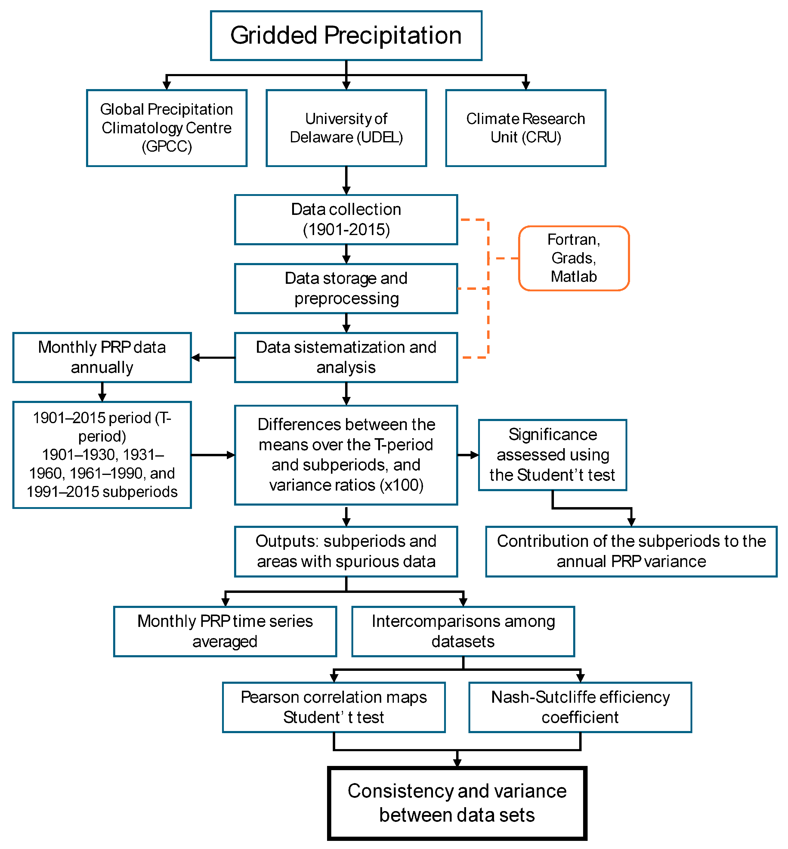
2. Materials and Methods

2.1. Study Area

The study area extends over most of continental SA (Figure 1) and is limited at 15.25° N, 55.25° S, 84.75° W, and 29.75° W. SA locates mostly in the Southern Hemisphere and is geographical boundaries: the Pacific Ocean to the west, North America and the Atlantic Ocean to the north and east, and the Caribbean Sea to the northwest (Figure 1). SA presents a geographical complexity, with the Andes Mountains along the Pacific coast being its main topographic relief (Figure 1). SA presents diverse ecosystems and climates that are influenced by geographical factors and teleconnections modulated by sea surface temperature variations occurring in the oceans at time scales varying from interannual to multidecadal [28]. The main geographical factors influencing the South American climate include the Andes Mountains, Amazon forest, Amazon and La Plata Basins, and Pantanal wetlands [28]. Flantua et al. [29] classified the continental SA into three major climate zones: tropical, subtropical and extratropical. The tropical zone is modulated by the seasonal migration of the intertropical convergence zone in the Pacific and Atlantic oceans, and the associated South American monsoon system; in the region to the east of the Andes, moisture is transported from the tropics to the subtropics by the Andean low-level jet and incursions of extratropical systems east of Andes affect the subtropical climate; the extratropical SA is modulated by a quasi-permanent westerly associated with the subtropical anticyclones in the Pacific and Atlantic oceans [29]. Under these influencing factors, SA comprises diverse climates across its vast landmass, with the Amazon rainforest transitioning into savannas in central Brazil, semi-arid regions such as in northeast Brazil, and temperate climate in southern regions.

2.2. Data Description

One hundred fifteen years (1901–2015) of monthly gridded PRP data from the GPCC, UDEL, and CRU were obtained for the study area, and in the same horizontal grid with a resolution of 0.5 degrees in latitude and longitude. The monthly CRU PRP data were based on PRP data from several agencies, including, among others, the National Meteorological Agencies (NMAs), the World Meteorological Organization (WMO), the CRU, the Centro Internacional de Agricultura Tropical, and the Food and Agriculture Organization (FAO). The CRU PRP data used here is version 4.0 obtained from the University of East Anglia Climatic Research Unity, available at: http://badc.nerc.ac.uk/ (accessed on 5 January 2023).
Several sources of PRP data integrate the GPCC collecting and processing system, among others: the NMAs (primary data source), the daily surface synoptic observations and monthly climate messages from the WMO Global Telecommunication System, the global PRP data from the CRU, FAO, and Global Historical Climatology Network (GHCN) at the National Centers for Environmental Information, such that the GPCC includes information from more than 85,000 stations worldwide. The GPCC, using a high-quality control system, produces four global gridded monthly PRP products; we use the GPCC Full Data Reanalysis V.8 version available at http://www.dwd.de (accessed on 27 May 2022) [13].
The UDEL dataset was constructed using data from several sources, including the GHCN (version GHCN2 and GHCN-daily), the Atmospheric Environment Service/Environment Canada archive, the Hydro-meteorological Institute in St. Petersburg, Russia, the Greenland Climate Network data, and daily records from the Global Surface Summary of the Day, Webber, and Willmott’s South American monthly precipitation station records, among others. The UDEL PRP data used in the present analysis refer to the version 5.01 dataset [15], provided by the University of Delaware from their website at http://climate.geog.udel.edu/~climate/html_pages/ (accessed on 21 September 2020).
These gridded datasets were constructed with different methods of spatial interpolation from the gauge-station data. The CRU data are obtained from the angular-distance weighted (ADW) interpolation scheme proposed by Shepard [30]. In this method, the data of eight gauge stations within a correlation-decay distance to the grid point are used; for grid points with no station within a correlation-decay distance, the climatological mean value is imposed. Consequently, in some areas with sparse distribution of the meteorological stations, the interpolated value can be invariant over a number of years. The GPCC data were interpolated with a spherical adaptation of the ADW method, which was developed by Willmott et al. [31]. The UDEL data were also obtained with the spherical ADW scheme in combination with the Climatologically Aided Interpolation (CAI) method [32], in which a spatially high-resolution climatology is used to calculate the monthly PRP difference at each station. Using the spherical ADW method, these differences are interpolated to the grid points. Then, in each grid point, the corresponding climatological value and monthly difference are added.
Figure 2 illustrates the flowchart followed in the data collection presented above, including the calculations and methods carried out in the research, which are explained in the following section.

2.3. Methods

2.3.1. Analyses for Individual Dataset

For each dataset, the annual PRP time series is obtained in each grid point by accumulating the monthly PRP data annually. For each grid point, the means of annual PRP are calculated considering the 1901–2015 period (T-period) and the 1901–1930, 1931–1960, 1961–1990, and 1991–2015 subperiods. The patterns of the differences between the means of annual PRP over the T-period and subperiods are examined. Since these differences are between the T-period and subperiods, the significant positive (negative) differences indicate that the PRP values during the subperiod are lower (greater) than those during the T-period, such that the subperiod contributes to reducing (increasing) the means of the T-period.
Also, the variance ratios of the annual PRP of the T-period and of the subperiods are examined. In this case, for each grid point, the variance for each subperiod is regarding the corresponding mean of the annual PRP of the T-period. In each grid point, the ratio of the subperiod variance and the T-period variance multiplied by 100 is obtained. These ratios indicate the percentage of the PRP variance during the T-period explained by the subperiods, so that areas with ratios less (greater) than 100% indicate lower (higher) PRP variability in those areas during the subperiod than during the T-period. For each dataset, analyses of the differences between the means of annual PRP over T-period and subperiods and variance ratios allow the identification of subperiods and areas with possible spurious data, or replacement of missing data by climatological data.
It will be clear in the results that two areas with possible spurious data could be identified, one in central Brazil (CBR) with limits at 55.25° W, 49.25° W, 17.75° S, and 12.25° S, and the other in central Bolivia (CBO) with limits at 66.75° W, 62.75° W, 17.75° S, and 15.25° S. For comparisons, three additional areas without apparent spurious data are also selected. In these cases, the selection is based on distinct climate features of three areas: one in central eastern Amazon (CAM) bounded at 70.25° W, 50.25° W, 11.75° S, and 0.25° N, the second in NEB with limits at 45.25° W, 35.25° W, 10.25° S, and 5.25° S, and the last in SESA bounded at 60.25° W, 50.25° W, 35.25° S, and 22.25° S. The locations of these areas are illustrated in Figure 1. The monthly PRP time series averaged in each area was obtained separately for each dataset and plotted in a month-versus-year graphic.
The significance of the differences between the means of the annual PRP values over the T-period and subperiods is assessed using Student’s t test. Considering two variables X 1 and X 2 with n 2 and n 1 values, S 1 and S 2 standard deviations, X 1 ¯ and X 2 ¯ respectively, and that the difference X 1 ¯ X 2 ¯ has a Student-t distribution, the absolute values of X 1 ¯ X 2 ¯ exceeding
t α n 1 + n 2 2   n 1 1 S 1 2 + ( n 2 1 ) S 2 2   n 1 + n 2 n 1 n 2 ( n 1 + n 2 2 )
where t α n 1 + n 2 2 is obtained in a Student’s t table for significance level α and n 1 + n 2 1   degrees of freedom are statistically significant [33]. The significance level of 0.05 is used in this test.

2.3.2. Intercomparisons among Datasets

Intercomparisons among the datasets are done with the annual PRP during the 1901–2015 period. Considering the three areas without apparent spurious data (CAM, NEB, and SESA), the differences of the annual cycles every two datasets (GPCC minus CRU, GPCC minus UDEL, and UDEL minus CRU) are obtained.
Comparisons among the datasets are also performed using the correlation maps. Using the Pearson correlation coefficient, the correlation maps every two datasets are constructed. The significance of the correlation is tested using the Student’s t test. Considering two variables X 1 and X 2 with n values and the correlation coefficient r , the absolute values of r excedding
t α , n 2 2 n 2 + t α , n 2 2
where t α , n 2 is obtained in a Student’s t table for significance level α and n 2   degrees of freedom are statistically significant [33]. The significance level of 0.01 is used in this test.
Also, comparisons among the datasets are conducted by calculating the Nash–Sutcliffe efficiency coefficient of the annual PRP every two datasets. The Nash–Sutcliffe efficiency coefficient was first used to assess the predictive skill of hydrological models, and is defined as one minus the ratio of the error variance of the modeled time series to the variance of the observed time series. Here, we consider the NSE to evaluate the degree to which one gridded precipitation dataset reproduces another dataset. So, considering the annual PRP as P this coefficient is obtained after Nash and Sutcliffe [34] as:
N S E = 1 t = 1 T P 1 t P 2 t 2 t = 1 T P 1 t P 1 ¯ 2
where P 1 ¯ is the mean of annual PRP for precipitation dataset 1, P 1 t and P 2 t are, respectively, the annual PRP for datasets 1 and 2 at time t . NSE varies from to 1. Interpretation of NSE values are: N S E = 0 means that the error variance of the dataset 2 time series is equal to the variance of the dataset 1 time series; N S E < 0 ; indicates that the error variance of the dataset 2 time series exceeds the variance of the dataset 1 time series; and NSE close to 1 indicates better agreement between datasets.

3. Results

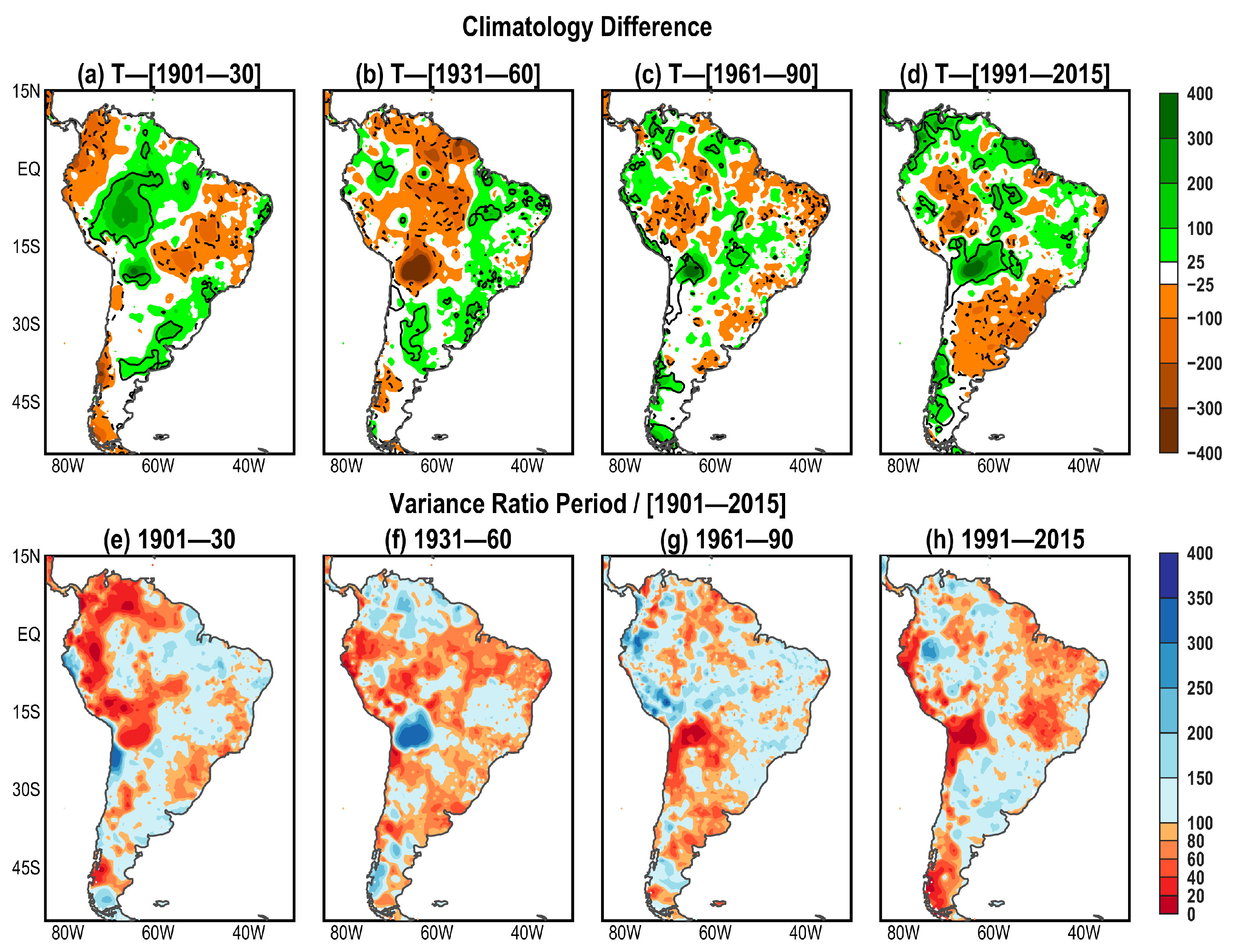
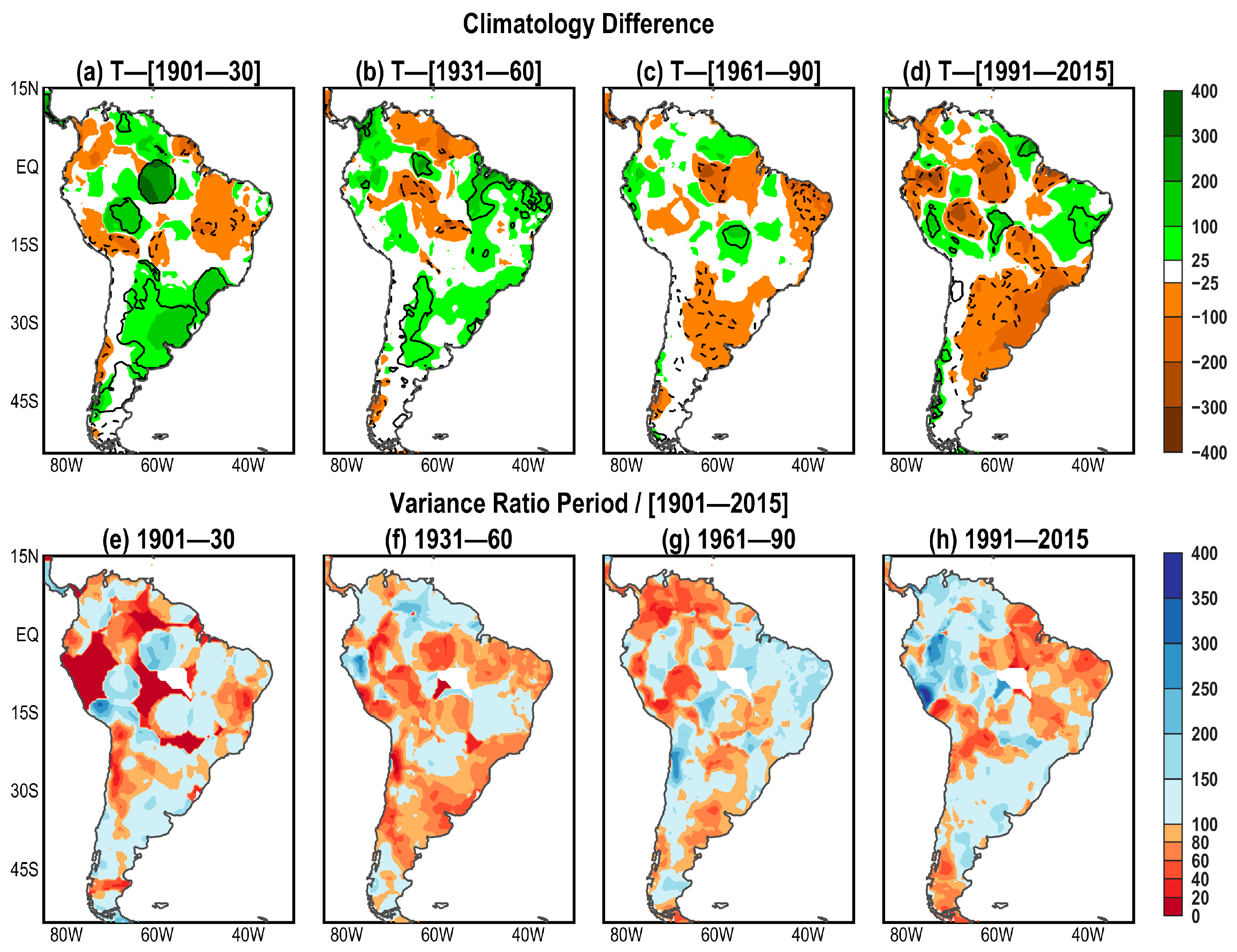
3.1. Comparisons between the T-Period (1901–2015) and the Subperiods of the Mean and Variance of the Annual PRP

3.1.1. GPCC

The GPCC differences between the means of the annual PRP of the T-period and the subperiods are illustrated in Figure 3a–d. For the T-[1901–1930] map, non-significant absolute values less than 50 mm are found in most of tropical SA, except for significant negative differences in small scattered areas in NEB, and in two small areas, one in central-eastern Brazil (centered around 10° S; 47° W) and another in central-western Chile (Figure 3a). Also, significant positive differences are found in an area extending from eastern Paraguay to eastern subtropical Argentina. Thus, except in areas with significant differences, the 1901–1930 subperiod, in general, has a small contribution to the mean of the annual PRP of the T-period (Figure 3a). The T-[1931–1960] map shows significant positive values in areas along a narrow zone from central western Colombia to NEB, and in subtropical SA (central northern Argentina and southern Brazil), and negative ones in small areas in the central-southwestern Amazon along approximately 20° S, and in extratropical southern Chile around 50° S. Therefore, in specific tropical areas, the 1931–1960 subperiod has a relatively larger contribution than the 1901–1930 subperiod to the means of the annual PRP over the T-period (Figure 3b). On the other hand, the T-[1961–1990] map presents considerably reduced absolute differences in most of the tropics and extratropics, except for significant negative values in small areas scattered in central equatorial SA and southwestern Amazon (Figure 3c). Contrasting with the other three subperiods, the 1991–2015 subperiod shows larger areas with significant positive differences in equatorial SA to the north of 20° S and significant negative differences over southeastern Brazil and SESA (which includes southern Brazil, Uruguay, and eastern Argentina to the north of 40° S) (Figure 3d).
The GPCC variance ratios between the subperiods and the T-period are shown in Figure 3e–h. For the 1901–1930 subperiod, variance ratios less than 20% are found in extensive areas of tropical SA to the north of 20° S and west of approximately 50° W, in an area extending from central-western Brazil to Uruguay and in part of southeastern Brazil (Figure 3e). The small percentages reflect reduced PRP variability in these areas during the 1901–1930 period, which might be due to the sparse distribution of the meteorological stations in tropical SA [13] and the consequent errors or approximations introduced in the interpolation procedure to produce the gridded data [8]. For the 1931–1960 subperiod, except for ratios less than 20% in southeastern Amazon and central Brazil, the ratios, in general, vary from 60% to 200%, with percentages between 60% and 100% from northern Brazil close to the mouth of the Amazon River to NEB, and in an extensive area from Ecuador across the southwestern Amazon to subtropical Argentina, and values above 100% in northwestern, northern, and extreme southern SA and some areas of eastern, central-western, and southern Brazil (Figure 3f). The percentage of less than 20% in southeastern Amazon and central Brazil might reflect the absence of data (see [35]). For the 1961–1990 subperiod, percentages exceeding 100% occur in most of tropical SA and extreme southern SA, and percentages less than 100% extend over central and western SA approximately between 20° S and 40° S (Figure 3g). For the 1991–2015 subperiod, ratios exceed 100% in most of SA, except for small areas in northwestern, northeastern, and southern SA and extreme western SA around 20° S (Figure 3h). The variance ratio maps indicate a gradual change in most of the tropical SA from reduced variability during the 1901–1930 subperiod to increased variability during the last two subperiods.

3.1.2. UDEL

The UDEL differences between the means of the annual PRP of the T-period and the subperiods are illustrated in Figure 4a–d. The T-[1901–1930] map shows significant negative values in western Colombia, central western Brazil, and central western Chile around 40° S, and significant positive values in a large area including southern Peru, northern Bolivia, and western Brazilian Amazon, and in small areas of southern Bolivia and northeastern and central eastern Argentina (Figure 4a). The T-[1931–1960] map depicts areas with significant negative values along a meridional zone from Guiana/Suriname/French Guiana to southwestern Bolivia, and significant positive values in small areas scattered over NEB, eastern Amazon, southeastern and southern Brazil, extreme western Brazilian Amazon, and central northern Argentina (Figure 4b). Comparing with the two previous described maps, the T-[1961–1990] map shows reduced magnitude differences, except for significant values in small areas scattered in southwestern and central northern Amazon with negative values, and in northwestern SA, in central western Brazil, and along western SA from 20° S to the south with positive values (Figure 4c). The 1991–2015 subperiod presents significant positive differences in a narrow band in northwestern SA, eastern Suriname, and French Guiana, in small areas in southeastern Amazon, southern Bolivia, northern Chile, and central Chile (around 40° S), and significant negative differences in southeastern Brazil, SESA, and western Brazilian Amazon (Figure 4d). Similar to those of the GPCC, the UDEL means of the annual PRP over SA vary depending on the subperiod, with the annual PRP in most of SESA evolving from drier conditions during the 1901–1930 subperiod to wetter conditions during the 1991–2015 subperiod. Nevertheless, the UDEL annual PRP in extensive areas of a meridional zone from Guiana/Suriname/French Guiana to southwestern Bolivia shows a reduction of the annual PRP from the 1931–1990 to 1991–2015 subperiod.
The UDEL variance ratios between the subperiods and the T-period are shown in Figure 4e–h. For the 1901–1930 subperiod, percentages less than 40% occur along areas over northern and western SA from central Venezuela to northern Chile and central Bolivia, and those between 60% and 80% along eastern Brazil, in central western Argentina around 30° S, and in southwestern SA around 45° S (Figure 4e). In the other areas, in general, percentages vary from 100% to 200%, except in two areas in western SA around 5° S and 25° S with percentages between 200% and 300% (Figure 4e). For 1931–1960 subperiod, percentages varying, in general, from 60% to 100% are noted in a near zonal band from Ecuador to NEB, along a narrow band from southwestern Amazon to southeastern Brazil around 22° S, in northern Chile, and in part of SESA (Figure 4f). These areas are permeated by areas with percentages varying from 100% to 200%, for an extensive area in northern SA; and most of Bolivia, with a variance ratio exceeding 200% (Figure 4f). For the 1961–1990 subperiod, small scattered areas with ratios of 60–100% permeate values exceeding 100% over SA north of 20° S; with values above 200% along west coast of SA from Ecuador to northern Chile; and with values less than 100% in the remaining areas of SA, with values less than 60% in western SA around 22° S (Figure 4g). For the 1991–2015 subperiod, values less than 100% occur in central northern Amazon, an area extending along the northern coast of SA from Suriname to NEB, and in central eastern Brazil, where the values vary from 20% to 60%, and percentages less than 60% are noted along the west coast of SA from Ecuador to northern Chile, where they extend over Bolivia and into the extreme southern SA (Figure 4h). In the complementary areas, the percentages vary mostly from 100% to 200%, except in the neighboring of southern Colombia and northern Peru with percentages above 200% (Figure 4h). The most outstanding feature in the variance ratio maps is the contrasting PRP variability over central Bolivia, which is reduced during the 1901–1931, 1961–1990, and 1991–2015 subperiods, and increased during the 1931–1960 subperiod (Figure 4e–h).

3.1.3. CRU

The CRU differences between the means of the annual PRP of the T-period and the subperiods are illustrated in Figure 5a–d. The T-[1901–1930] map shows significant positive values in large areas; one includes southern Peru and northern Bolivia, the second in central Amazon, and another one extends over southeastern Brazil, from SESA to most of the Argentinean territory. Meanwhile, negative differences, mainly varying from 0 to −100 mm, are noted in tropical SA in its central eastern side and along the western coast (Figure 5a). The T-[1931–1960] map for the CRU and the corresponding one for GPCC show similar patterns, except that the CRU’s pattern is smoother than the GPCC’s pattern (Figure 3b and Figure 5b). Also, the T-[1961–1990] map for the CRU and the corresponding one for the GPCC shows similarities, except for smoother patterns and an area in central-western Brazil with significant differences for CRU’s map (Figure 3c and Figure 5c). On the other hand, the T-[1991–2015] map for CRU presents significant negative differences of less than −100 mm in well-defined areas in equatorial Amazon, northern Bolivia, part of central-western Brazil, southeastern Brazil, SESA, and most of Argentina to the north of 45° S, and areas with significant positive differences along 15° S and over French Guiana (Figure 5d).
The CRU variance ratios between the subperiods and the T-period are shown in Figure 5e–h. For the 1901–1930 subperiod, percentages less than 20% are noticeable in central northern Amazon, northern Peru, and southwestern Amazon, and less than 100% along the eastern coast of Brazil to the north of 20° S, in tropical Chile, and in adjacent areas of western Argentina (Figure 5e). These areas with reduced percentages are permeated by ratios varying from 100% to 150% in most regions, with percentages reaching around 200% in southern Amazon and southern Peru (Figure 5e). The variance ratios for the 1931–1960 subperiod for the CRU and UDEL show similar patterns, except for the absence of values greater than 200% over Bolivia and reduced percentages over southern Ecuador and adjacent Peruvian areas replaced by percentages greater than 200% for the CRU (Figure 4f and Figure 5f). The percentages for the 1961–1990 subperiod are dominated by values less than 100% in northern SA, in central and southwestern Amazon, along the western coast of Peru, and in a narrow meridional band extending from central-western Brazil into part of SESA, which is permeated by percentages mostly between 100% and 200% (Figure 5g). For the 1991–2015 subperiod, percentages lower than 100% occur in a large area including Suriname, French Guiana, eastern Amazon, northern Brazil, NEB, southern Peru, northern Chile, part of Bolivia, and extreme southern SA, and percentages greater than 100% extend over SA north of 20° S and west of 60° W, part of central-western Brazil, and in most areas in SA to the south of 22° S. In all subperiods, there is an indication of absence of data in southeastern Amazon. Harris et al. [35] previously highlighted this aspect for the CRU dataset.

3.1.4. Analyses of Specific Areas

Analyses of the variance ratio maps indicate areas with possible spurious or missing data, for the GPCC an area in southeast Amazon and central Brazil, for the CRU in part of southeast Amazon, and for the UDEL a region in central Bolivia. The CBR and CBO areas whose geographical limits are defined in Section 2.3.1 and illustrated in Figure 1 overlap, respectively, the area identified in the GPCC and CRU and that in the UDEL. So, these two areas and the additional ones defined in Section 2.3.1 as CAM, NEB, and SESA are examined here.
The three timeseries for CBO show quite distinct temporal behaviors before approximately 1941 (Figure 6). The GPCC shows very reduced variability, with almost the same value for each month over the years from 1901 to 1932; then there is a gradual variability increase of the monthly values from 1932 to 1992 (Figure 6a). The UDEL depicts reduced variability of the monthly PRP over the years during the 1901–1928 period, and artificially increased monthly values from May to September of the years from 1929 to 1941, then the monthly PRP values from 1942 onwards show similar behavior as those corresponding to the GPCC (Figure 6a,b). The CRU shows greater variability of the monthly PRP values over the period of analysis than the other two datasets, with relatively larger variability before 1941 (Figure 6c). These results indicate that PRP analysis over central Bolivia for the periods approximately before 1941 should be undertaken with caution, particularly using the GPCC and UDEL datasets.
Another area with possible missing data, CBR, seems less problematic (Figure 7). Indeed, the UDEL and CRU datasets show consistent variability of the monthly PRP values over the period of analysis (Figure 7b,c). Nevertheless, the GPCC shows quite reduced variability of the monthly values over the years from 1901–1970 approximately and then a similar behavior as the other datasets (Figure 7). Thus, analysis of CBR for periods before 1970 with the GPCC should be undertaken with caution.
The CAM encompasses a large portion of the Amazon and is an area without apparent spurious data, but it is located in a region with sparce in situ observations (Figure 8). The UDEL and CRU time series present, in general, consistent monthly PRP variability, which is slightly smaller for the CRU during the austral months over all years and during all months for years before 1921. The GPCC discloses considerable reduced variability for all years, which is more pronounced before 1925.
For the time series in NEB and SESA (Figure 9 and Figure 10), consistent variability of the monthly PRP values is evident between UDEL and CRU during the period of analysis. Meanwhile, the GPCC presents less variability before 1940 in SESA, and before 1910 in NEB, than the corresponding time series for the UDEL and CRU.

3.2. Comparisons among the Datasets
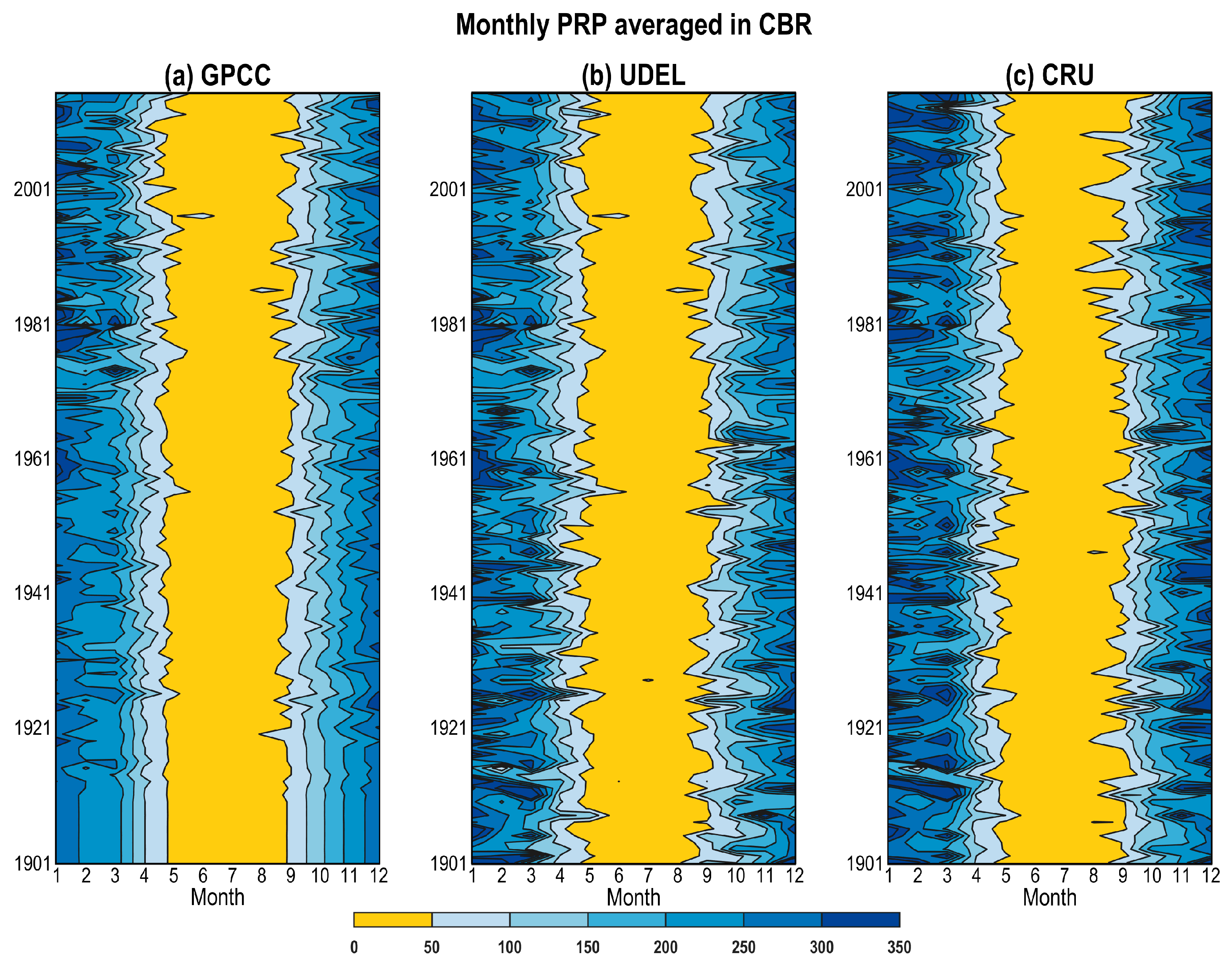
3.2.1. Annual Cycle

Comparisons among the datasets are done considering the annual cycles for the CAM, NEB, and SESA timeseries (Figure 11). The annual cycle differences every two datasets show the largest magnitudes in the CAM, notably between GPCC and UDEL and between UDEL and CRU during the months from May to September (Figure 11a). The smallest magnitudes of the annual cycle differences occur in NEB (Figure 11b). The magnitudes of these differences are also small in SESA, except in some isolated months, such as in November for the difference GPCC and CRU, and in October for the difference UDEL and CRU (Figure 11c).

3.2.2. Statistical Indicators

Maps of the correlations and Nash–Sutcliffe efficiency coefficient (NSE) exhibit consistent patterns (Figure 12). The correlation map between GPCC and UDEL shows values less than 0.65 in small areas in northwest SA, an area extending from southeastern Amazon to central Brazil, southwestern Amazon, central Bolivia, and along the coast of Peru (Figure 12a). It is worth mentioning that the areas in southeast Amazon and central Bolivia encompass non-significant correlations smaller than 0.25. Areas with correlations less than o.65 are permeated by larger correlations with values exceeding 0.85 in areas along eastern SA, which extends from the north coast of Brazil east of 50° W to central Argentina (Figure 12a). Areas with correlations less than 0.65 coincide with those with negative NSE and those with correlations exceeding 0.85 with those with NSE greater than 0.8 (Figure 12a,d).
For the GPCC and UDEL, correlations less than 0.65 or NSE negative occur in a large area including the entire Amazon Basin, which extends northwest and northward into eastern Colombia, southern Venezuela, Guiana, Suriname and French Guiana and southeastward into part of southeast Brazil (Figure 12b,e). Also, non-significant correlations are noted in extensive areas of the Amazon region. Correlations exceeding 0.85 or NSE values greater than 0.8 are found over northeast and southeast SA Figure 12b,e).
The correlation map between the UDEL and CRU features correlations less than 0.65 in an extensive area encompassing the southern and northern sector of the Amazon, eastern Colombia, eastern Peru, central Bolivia, and central eastern Brazil (Figure 12c). In this case, non-significant correlations are noted in two well-defined areas, one in southeastern Amazon and central Brazil and another in central Bolivia. Correlations greater than 0.85 occur in areas of northeast SA, southern Brazil, Uruguay, and eastern Argentina (Figure 12c). The consistencies between correlation and NSE patterns are conspicuous (Figure 12c,f)

4. Discussion

Intercomparisons of the PRP data from the GPCC, UDEL, and CRU datasets over SA for the 1901–2015 period are conducted concerning the annual means and variances, monthly values in selected areas, annual cycles, and statistical indicators. The means of the annual PRP in some regions in SA depend strongly on the subperiod (Figure 4a–d, Figure 5a–d and Figure 6a–d). Some regions show long-term evolving PRP patterns that reflect the PRP trends. In this regard, Zhou et al. [36] previously reported, in the global context, positive trends in rainy areas and negative trends in dry areas for the 1979–2007 period. This relationship of the trend signs and the regional PRP climate conditions is evident in SESA, southeastern Brazil, and NEB (Figure 4a–d, Figure 5a–d and Figure 6a–d). In the case of SESA and southeastern Brazil, all three datasets show gradual evolving features from less to more rainy conditions from 1901–1930 to the 1991–2015 subperiod. Thus, the positive PRP trend in SESA and southeastern Brazil documented earlier for shorter periods such as 1960–2000 [37], 1955–2004 [28], 1981–2021 [38], and 1950–2020 [39] is part of a secular positive PRP trend. For the NEB, all three datasets show negative PRP trends during two distinct periods: 1901–1960 and 1961–2015. In such a case, the PRP evolving feature might reflect the joint action of the Pacific Decadal Oscillation and Atlantic Multidecadal Oscillation in modulating the PRP in a multidecadal time scale [24]. However, the negative PRP trend in NEB during the 1961–2015 period is consistent with previous finding by Shimizu et al. [12], who used the PRP data from the Climate Prediction Center (CPC) Merged Analysis of Precipitation (CMAP) during the 1981–2019 period. They found an increased PRP trend along the river basins located in eastern NEB.
The Amazon region is another interesting region to be considered in isolation here. It presents a wetting trend during the 1901–2015 period, which is noticeable in the central western sector for the UDEL and slightly to the east in the central Amazon for the CRU; and no apparent trend is noted for the GPCC. It is worth mentioning that the wetting trend for the CRU data extends over the eastern and western Amazon sectors during 1991–2015. The wetting pattern noted for the CRU dataset is supported by earlier analysis using in situ observations [40]. These authors, using time records spanning over almost 80 years starting in the 1920s, found positive PRP trends at Barcelos, Manaus, Belém, and Soure, which are surface stations located in the central and eastern Amazon. However, the non-significant trends in most analyzed stations lead them to an unconclusive statement regarding the PRP trends in the Amazon. In this same sense, Costa and Foley [9], using data of the 1976–1996 period, argued that the PRP in the Amazon does not present a significant trend. Their conclusion might be biased by using the averaged PRP over the entire Amazon region. Nonetheless, coherently with the more extensive wetting pattern noted in the Amazon for the CRU dataset during 1991–2015, several earlier studies documented PRP increase in parts of the Amazon basin starting in early 1990s during the wet season (December to May) [41,42,43]. In addition, Shimizu et al. [12] found an increased PRP trend along the river basins located in the north and west of the Brazilian Amazon region during 1981–2019. Therefore, the means of the PRP in the Amazon region show spatiotemporal differences depending on the period of analysis, dataset, and subregions.
The contributions of the subperiods to the PRP variance during the T-period show differences among datasets. The GPCC shows a gradual change of the variance ratio pattern, starting with dominantly small values in an extensive area of most of the tropical SA to the west of 50° W and north of 20° S, and sectors of southeast Brazil and central eastern SA, during the 1901–1930 subperiod, which are replaced by greater values during the last two subperiods (Figure 3e–h). This extensive area includes the CBR, CBO, CAM, and part of SESA, where the monthly PRP time series show reduced variability before 1940 (Figure 4a, Figure 7a, Figure 8a and Figure 10a). In addition, the abovementioned tropical SA area overlaps that with poor coverage of surface meteorological stations [13]; due to that, the interpolation procedure system between rain-gauge locations to get gridded data might introduce errors [8]. Therefore, the studies on the PRP variability using the GPCC data for long periods, including data of the 1901–1930 period, might be biased due to the reduced variability during this period over a large extension of SA.
For the UDEL and CRU datasets, the reduced contribution of the 1901–1930 to the PRP variance during the T-period is confined to relatively small areas of the tropical SA (Figure 4e and Figure 5e). For the CRU, they occur in areas in the Amazon and central eastern Brazil; for the UDEL, they extend over northern and western SA from central Venezuela to northern Chile and central Bolivia. Considering the UDEL, the PRP variability in the CBO is also reduced during the 1961–1990 and 1991–2015 subperiods and increased during the 1931–1960 subperiod (Figure 4e–h). This feature is not noted for the GPCC and CRU datasets (Figure 3e–h and Figure 5e–h). Examination of the CBO monthly PRP time series for the UDEL indicates reduced monthly PRP variability over the years from 1901 to 1928, and artificially increased monthly values from May to September of the years from 1929 to 1941. Careful manual inspections of the monthly PRP time series in the grid points within the CBO area reveal, in most grid points, that the UDEL presents an order of magnitude larger than the corresponding values of the other datasets. Since the PRP unit in the UDEL is cm [15] we believe that in some stations within the CBO area, the PRP was reported in mm. For variability analysis using the UDEL PRP dataset, if the period of interest would include the years from 1929 to 1941, among others, the monthly (from May to September), seasonal (those that include May to September months), and yearly anomalies would be overestimated for the years from 1929 to 1941 (positive values) and underestimated for the other years (negative values) over the CBO area. These contrasting positive/negative anomalies over the CBO area would not depend on the period taken as a reference for climatology. Therefore, using the UDEL PRP dataset, analysis over central Bolivia for periods before approximately 1940 should be undertaken with caution.
In addition, analyses of the variance ratio maps for the CRU indicate missing data in southeastern Amazon in all subperiods, as previously highlighted by Harris et al. [35]. The CBR time series includes this area and part of central Brazil. Analyses of the UDEL and CRU time series in CBR show consistent variability of the monthly PRP values over the period of analysis, but the corresponding GPCC time series shows quite reduced variability of the monthly values over the years from 1901 to 1970 approximately. Thus, analysis over CBR for periods before 1970 with the GPCC should be taken with caution.
Regarding the annual cycles in CAM, NEB, and SESA with the reference period of 1901–2015, the large differences among the datasets occur for the CAM (Figure 11). For this dataset, the large differences occur during the months from May to September, which overlaps with months of the dry-season in the Amazon (from June to September) when the PRP is less than 100 mm [9]. The magnitude of these differences varies from 10 to 15 mm, which is not negligible regarding the seasonal value. Negrón-Juarez et al. [10] found among six datasets, including the GPCC, coherent PRP seasonal cycles over the Amazon Basin for the 1986–2005 period. In addition, the CAM is in an area with sparse distribution of stations [13,15] and the use of a long reference period in our analysis is likely the source of not-negligible differences. The small differences in the annual cycle among the datasets for NEB and SESA are in agreement with previous studies [10,11].
Analyses every two dataset show coherent results for the two statistical indicators, such that correlations less than 0.65 and negative NSE occur in almost the same areas, as well as correlations exceeding 0.85 and NSE greater than 0.8 (Figure 12). Correlations less than 0.65 (or negative NSE) are found in tropical SA mostly to the west of 50° W and north of 20° S, which is an area with poor coverage of in situ surface observations [13,15]. In the complementary areas, correlations exceeding 0.85 (NSE greater than 0.8) are noted in northeast SA, southeast SA, and southern Brazil, which are areas with high coverage of surface stations [13,15]. Correlations (NSE) between the GPCC and CRU less that 0.65 (negative) occur in more extensive areas than between the GPCC and UDEL and between the UDEL and CRU. Therefore, studies using these datasets might present coherent results among them in areas along eastern SA, whereas in western SA, particularly north of 20° S, discrepancies might occur.

5. Conclusions

In the present analysis we provide intercomparisons of the PRP data from the GPCC, UDEL, and CRU datasets over SA for the 1901–2015 period. The means of the annual PRP in some regions of SA show long-term evolving patterns. For SESA and southeastern Brazil, all three datasets show gradual evolving features from less to more rainy conditions from 1901–1930 to the 1991–2015 subperiod. For the NEB, all three datasets show negative PRP trends during two periods: 1901–1960 and 1961–2015, which might reflect the joint action of the Pacific Decadal Oscillation and Atlantic Multidecadal Oscillation modulating the PRP in a multidecadal time scale. The Amazon region depicts a wetting trend during the 1901–2015 period in its central western sector for the UDEL and in the central Amazon for the CRU. Therefore, the means of the annual PRP in SESA and southeastern Brazil, NEB, and parts of the Amazon depend strongly on the subperiod. This result has implications for climate variability analyses, for which anomalies are calculated using a reference period of, in general, 30 years. The use of a reference period shorter than the study period should be avoided, due to the differences in the subperiod illustrated here.
Analyses of the contribution of the subperiods to the annual PRP variance during the 1901–2015 period indicate, for the GPCC, dominantly small values in an extensive area of the tropical SA to the west of 50° W and north of 20° S and sectors of southeast Brazil and central eastern SA during 1901–1930. Also, this area overlaps that with poor coverage of surface meteorological stations. The results indicate that the interpolation procedure system between rain-gauge locations to obtain gridded data might have introduced errors. Therefore, the studies on the PRP variability using the GPCC data for long periods, including the data of the 1901–1930 period, might take into consideration the reduced variability, during this period, over a large extension of SA.
We found an area in central Bolivia with possible spurious data for the UDEL. The CBO monthly time series presents reduced monthly PRP variability over the years from 1901 to 1928, and artificially increased values in the months from May to September of the years from 1929 to 1941. We believe that, in some stations within the CBO area, the PRP was reported in mm. For variability analysis, if the period of interest includes the years from 1929 to 1941, among others, the monthly anomalies in the months from May to September would be overestimated for the years from 1929 to 1941 and underestimated for the other years over the CBO area. Since these biased anomalies might affect the results, analyses using the UDEL dataset including periods before 1941 should be considered with caution.
The two statistical indicators present coherent results. Correlations less than 0.65 (or negative NSE) are found in areas with poor coverage of in situ surface observations, and correlations exceeding 0.85 (NSE greater than 0.8), in areas with high coverage of surface stations. Therefore, the datasets might present coherent results among them in areas along eastern SA, whereas in western SA, particularly north of 20S, discrepancies might occur.
Due to some differences among the datasets reported in the present analysis, separated analyses with two datasets might be desired depending on the objective of the studies involving PRP in SA. We also believe that the analyses presented here for the GPCC, CRU, and UDEL PRP datasets might be useful for future climate variability studies.

Author Contributions

Conceptualization, M.T.K.; Methodology, M.T.K., W.L.C. and R.V.A.; software, M.T.K. and W.L.C.; validation, M.T.K., W.L.C., R.V.A. and R.A.F.S.; formal analysis, M.T.K., W.L.C., R.V.A., R.A.F.S., M.H.S., L.C.M.J. and I.P.S.; investigation, M.T.K., W.L.C., R.V.A., R.A.F.S., M.H.S., L.C.M.J. and I.P.S.; resources R.V.A.; data curation, M.T.K., W.L.C. and R.V.A.; writing—original draft preparation, M.T.K.; writing—review and editing, M.T.K., W.L.C., R.V.A. and R.A.F.S. visualization, M.T.K.; supervision, M.T.K.; funding acquisition, R.V.A. All authors have read and agreed to the published version of the manuscript.

Funding

This work was partially supported by the Conselho Nacional de Desenvolvimento Científico e Tecnológico (CNPq) of Brazil [grant number 308435/2022-2].

Institutional Review Board Statement

Not applicable.

Informed Consent Statement

Not applicable.

Data Availability Statement

The data are contained within the article.

Acknowledgments

The first author thanks to the Universidade do Estado do Amazonas (UEA) for the Senior Visitor Researcher grant. The second author was supported by the Universidad del Valle (Cali-Colombia). We thank two reviewers for their helpful suggestions.

Conflicts of Interest

The authors declare no conflicts of interest. The founding sponsors had no role in the design, analysis, and interpretation of data; the writing manuscript; or the decision to publish the results.

References

  1. Trenberth, K.E.; Dai, A.; Rasmussen, R.M.; Parsons, D.B. The Changing Character of Precipitation. Bull. Am. Meteorol. Soc. 2003, 84, 1205–1217+1161. [Google Scholar] [CrossRef]
  2. Kidd, C.; Huffman, G. Global Precipitation Measurement. Meteorol. Appl. 2011, 18, 334–353. [Google Scholar] [CrossRef]
  3. Mesa-Sánchez, Ó.J.; Peñaranda-Vélez, V.M. Complejidad de La Estructura Espacio-Temporal de La Precipitación. Rev. Acad. Colomb. Cienc. Exactas Físicas Nat. 2015, 39, 304–320. [Google Scholar] [CrossRef]
  4. Chou, C.; Neelin, J.D. Mechanisms of Global Warming Impacts on Robustness of Tropical Precipitation Asymmetry. J. Clim. 2004, 17, 2688–2701. [Google Scholar] [CrossRef]
  5. Seneviratne, S.I.; Zhang, X.; Adnan, M.; Badi, W.; Dereczynski, C.; Di Luca, A.; Ghosh, S.; Iskandar, I.; Kossin, J.; Lewis, S.; et al. Chapter 11: Weather and Climate Extreme Events in a Changing Climate. In Climate Change 2021: The Physical Science Basis. Contribution of Working Group I to the Sixth Assessment Report of the Intergovernmental Panel on Climate Change; Masson-Delmotte, V., Zhai, P., Pirani, A., Connors, S.L., Péan, C., Berger, S., Caud, N., Chen, Y., Goldfarb, L., Gomis, M.I., et al., Eds.; Cambridge University Press: Cambridge, UK, 2021; p. 345. [Google Scholar]
  6. Sun, Q.; Miao, C.; Duan, Q.; Ashouri, H.; Sorooshian, S.; Hsu, K.L. A Review of Global Precipitation Data Sets: Data Sources, Estimation, and Intercomparisons. Rev. Geophys. 2018, 56, 79–107. [Google Scholar] [CrossRef]
  7. Carvalho, L.M.V. Assessing Precipitation Trends in the Americas with Historical Data: A Review. Wiley Interdiscip. Rev. Clim. Chang. 2020, 11, e627. [Google Scholar] [CrossRef]
  8. Gehne, M.; Hamill, T.M.; Kiladis, G.N.; Trenberth, K.E. Comparison of Global Precipitation Estimates across a Range of Temporal and Spatial Scales. J. Clim. 2016, 29, 7773–7795. [Google Scholar] [CrossRef]
  9. Costa, M.H.; Foley, J.A. A Comparison of Precipitation Datasets for the Amazon Basin. Geophys. Res. Lett. 1998, 25, 155–158. [Google Scholar] [CrossRef]
  10. Negrón Juárez, R.I.; Li, W.; Fernandes, K.; de Oliveira Cardoso, A. Comparison of Precipitation Data Sets over the Tropical South American and African Continents. J. Hydrometeorol. 2009, 10, 289–299. [Google Scholar] [CrossRef]
  11. Gulizia, C.; Camilloni, I. A Spatio-Temporal Comparative Study of the Representation of Precipitation over South America Derived by Three Gridded Data Sets. Int. J. Climatol. 2016, 36, 1549–1559. [Google Scholar] [CrossRef]
  12. Shimizu, M.H.; Anochi, J.A.; Kayano, M.T. Precipitation Patterns over Northern Brazil Basins: Climatology, Trends, and Associated Mechanisms. Theor. Appl. Climatol. 2022, 147, 767–783. [Google Scholar] [CrossRef]
  13. Schneider, U.; Becker, A.; Finger, P.; Meyer-Christoffer, A.; Ziese, M.; Rudolf, B. GPCC’s New Land Surface Precipitation Climatology Based on Quality-Controlled in Situ Data and Its Role in Quantifying the Global Water Cycle. Theor. Appl. Climatol. 2014, 115, 15–40. [Google Scholar] [CrossRef]
  14. Harris, I.; Jones, P.D.; Osborn, T.J.; Lister, D.H. Updated High-Resolution Grids of Monthly Climatic Observations—The CRU TS3.10 Dataset. Int. J. Climatol. 2014, 34, 623–642. [Google Scholar] [CrossRef]
  15. Willmott, C.J.; Matsuura, K. Global (Land) Precipitation and Temperature; Center for Climatic Research, Department of Geography, University of Delaware: Newark, NJ, USA, 2023; Available online: https://climatedataguide.ucar.edu/climate-data/global-land-precipitation-and-temperature-willmott-matsuura-university-delaware (accessed on 19 February 2024).
  16. Marengo, J.A. Interdecadal Variability and Trends of Rainfall across the Amazon Basin. Theor. Appl. Climatol. 2004, 78, 79–96. [Google Scholar] [CrossRef]
  17. Andreoli, R.V.; Kayano, M.T. ENSO-Related Rainfall Anomalies in South America and Associated Circulation Features during Warm and Cold Pacific Decadal Oscillation Regimes. Int. J. Climatol. 2005, 25, 2017–2030. [Google Scholar] [CrossRef]
  18. Kayano, M.T.; Andreoli, R.V. Relations of South American Summer Rainfall Interannual Variations with the Pacific Decadal Oscillation. Int. J. Climatol. 2007, 27, 531–540. [Google Scholar] [CrossRef]
  19. Jury, M.R. An Interdecadal American Rainfall Mode. J. Geophys. Res. Atmos. 2009, 114, 1–11. [Google Scholar] [CrossRef]
  20. Kayano, M.T.; Capistrano, V.B. How the Atlantic Multidecadal Oscillation (AMO) Modifies the ENSO Influence on the South American Rainfall. Int. J. Climatol. 2014, 34, 162–178. [Google Scholar] [CrossRef]
  21. Dong, B.; Dai, A. The Influence of the Interdecadal Pacific Oscillation on Temperature and Precipitation over the Globe. Clim. Dyn. 2015, 45, 2667–2681. [Google Scholar] [CrossRef]
  22. Kayano, M.T.; Andreoli, R.V.; Souza, R.A.F. El Niño–Southern Oscillation Related Teleconnections over South America under Distinct Atlantic Multidecadal Oscillation and Pacific Interdecadal Oscillation Backgrounds: La Niña. Int. J. Climatol. 2019, 39, 1359–1372. [Google Scholar] [CrossRef]
  23. Kayano, M.T.; Andreoli, R.V.; Souza, R.A.F. Pacific and Atlantic Multidecadal Variability Relations to the El Niño Events and Their Effects on the South American Rainfall. Int. J. Climatol. 2020, 40, 2183–2200. [Google Scholar] [CrossRef]
  24. He, Z.; Dai, A.; Vuille, M. The Joint Impacts of Atlantic and Pacific Multidecadal Variability on South American Precipitation and Temperature. J. Clim. 2021, 34, 7959–7981. [Google Scholar] [CrossRef]
  25. Prado, L.F.; Wainer, I.; Yokoyama, E.; Khodri, M.; Garnier, J. Changes in Summer Precipitation Variability in Central Brazil over the Past Eight Decades. Int. J. Climatol. 2021, 41, 4171–4186. [Google Scholar] [CrossRef]
  26. Kamae, Y.; Li, X.; Xie, S.P.; Ueda, H. Atlantic Effects on Recent Decadal Trends in Global Monsoon. Clim. Dyn. 2017, 49, 3443–3455. [Google Scholar] [CrossRef]
  27. Garreaud, R.D.; Vuille, M.; Compagnucci, R.; Marengo, J. Present-Day South American Climate. Palaeogeogr. Palaeoclimatol. Palaeoecol. 2009, 281, 180–195. [Google Scholar] [CrossRef]
  28. de Barros Soares, D.; Lee, H.; Loikith, P.C.; Barkhordarian, A.; Mechoso, C.R. Can Significant Trends Be Detected in Surface Air Temperature and Precipitation over South America in Recent Decades? Int. J. Climatol. 2017, 37, 1483–1493. [Google Scholar] [CrossRef]
  29. Flantua, S.G.A.; Hooghiemstra, H.; Vuille, M.; Behling, H.; Carson, J.F.; Gosling, W.D.; Hoyos, I.; Ledru, M.P.; Montoya, E.; Mayle, F.; et al. Climate Variability and Human Impact in South America during the Last 2000 Years: Synthesis and Perspectives from Pollen Records. Clim. Past 2016, 12, 483–523. [Google Scholar] [CrossRef]
  30. Shepard, D. Two- Dimensional Interpolation Function for Irregularly- Spaced Data. In Proceedings of the 23rd ACM National Conference, New York, NY, USA, 27–29 August 1968; pp. 517–524. [Google Scholar] [CrossRef]
  31. Willmott, C.J.; Rowe, C.M.; Philpot, W.D. Small-Scale Climate Maps: A Sensitivity Analysis of Some Common Assumptions Associated with Grid-Point Interpolation and Contouring. Am. Cartogr. 1985, 12, 5–16. [Google Scholar] [CrossRef]
  32. Willmott, C.J.; Robeson, S.M. Climatologically Aided Interpolation (CAI) of Terrestrial Air Temperature. Int. J. Climatol. 1995, 15, 221–229. [Google Scholar] [CrossRef]
  33. Wilks, D.S. Statistical Methods in the Atmospheric Sciences, 3rd ed.; Wilks, D.S., Ed.; Academic Press: San Diego, CA, USA, 2011; ISBN 9780123850232. [Google Scholar]
  34. Nash, J.E.; Sutcliffe, J.V. River Flow Forecasting through Conceptual Models Part I—A Discussion of Principles. J. Hydrol. 1970, 10, 282–290. [Google Scholar] [CrossRef]
  35. Harris, I.; Osborn, T.J.; Jones, P.; Lister, D. Version 4 of the CRU TS Monthly High-Resolution Gridded Multivariate Climate Dataset. Sci. Data 2020, 7, 109. [Google Scholar] [CrossRef] [PubMed]
  36. Zhou, Y.P.; Xu, K.M.; Sud, Y.C.; Betts, A.K. Recent Trends of the Tropical Hydrological Cycle Inferred,Fromglobal Precipitation Climatology Project and International Satellite Cloud Climatology Project Data. J. Geophys. Res. Atmos. 2011, 116, 1–16. [Google Scholar] [CrossRef]
  37. Haylock, M.; Peterson, T.C.; Alves, L.M.; Ambrizzi, T.; Anunciação, M.T.; Baez, J.; Barros, V.R.; Berlato, M.A.; Bidegain, M.; Coronel, G.; et al. Trends in Total and Extreme South American Rainfall in 1960–2000 and Links with Sea Surface Temperature. J. Clim. 2006, 19, 1490–1512. [Google Scholar] [CrossRef]
  38. Cerón, W.L.; Kayano, M.T.; Andreoli, R.V.; Avila-Diaz, A.; Ayes, I.; Freitas, E.D.; Martins, J.A.; Souza, R.A.F. Recent Intensification of Extreme Precipitation Events in the La Plata Basin in Southern South America (1981–2018). Atmos. Res. 2021, 249, 105299. [Google Scholar] [CrossRef]
  39. Varuolo-Clarke, A.M.; Williams, A.P.; Smerdon, J.E.; Ting, M.; Bishop, D.A. Influence of the South American Low-Level Jet on the Austral Summer Precipitation Trend in Southeastern South America. Geophys. Res. Lett. 2022, 49, e2021GL096409. [Google Scholar] [CrossRef]
  40. Satyamurty, P.; De Castro, A.A.; Tota, J.; Da Silva Gularte, L.E.; Manzi, A.O. Rainfall Trends in the Brazilian Amazon Basin in the Past Eight Decades. Theor. Appl. Climatol. 2010, 99, 139–148. [Google Scholar] [CrossRef]
  41. Gloor, M.; Brienen, R.J.W.; Galbraith, D.; Feldpausch, T.R.; Schöngart, J.; Guyot, J.L.; Espinoza, J.C.; Lloyd, J.; Phillips, O.L. Intensification of the Amazon Hydrological Cycle over the Last Two Decades. Geophys. Res. Lett. 2013, 40, 1729–1733. [Google Scholar] [CrossRef]
  42. Marengo, J.A.; Espinoza, J.C. Extreme Seasonal Droughts and Floods in Amazonia: Causes, Trends and Impacts. Int. J. Climatol. 2016, 36, 1033–1050. [Google Scholar] [CrossRef]
  43. Barichivich, J.; Gloor, E.; Peylin, P.; Brienen, R.J.W.; Schöngart, J.; Espinoza, J.C.; Pattnayak, K.C. Recent Intensification of Amazon Flooding Extremes Driven by Strengthened Walker Circulation. Sci. Adv. 2018, 4, 1–7. [Google Scholar] [CrossRef]
Figure 1. South America (SA) and its main features. Topography was obtained from the Shuttle Radar Topography Mission (SRTM), available at http://www2.jpl.nasa.gov/srtm/ accessed on 1 April 2024. Boundaries of the South American countries are indicated by black lines. Boxes limit the areas used in the analyses.
Meteorology 03 00009 g001
Figure 2. Methodological flowchart. The red box refers to computational languages used, the blue boxes give the followed steps, and the black box the final achievement.
Meteorology 03 00009 g002
Figure 3. Global Precipitation Climatology Centre (GPCC) differences between the means of the annual PRP of the T-period and the: (a) 1901–1930 subperiod; (b) 1931–1960 subperiod; (c) 1961–1990 subperiod; and (d) 1991–2015 subperiod. GPCC variance ratios between the subperiod and the T-period for: (e) 1901–1930; (f) 1931–1960; (g) 1961–1990; (h) 1991–2015. Units in (ad) are in mm. The values in (eh) are in percentages.
Meteorology 03 00009 g003
Figure 4. University of Delaware (UDEL) differences between the means of the annual PRP of the T-period and the: (a) 1901–1930 subperiod; (b) 1931–1960 subperiod; (c) 1961–1990 subperiod; and (d) 1991–2015 subperiod. GPCC variance ratios between the subperiod and the T-period for: (e) 1901–1930; (f)1931–1960; (g) 1961–1990; (h) 1991–2015. Units in (ad) are in mm. The values in (eh) are in percentages.
Meteorology 03 00009 g004
Figure 5. Climate Research Unit (CRU) differences between the means of the annual PRP of the T-period and the: (a) 1901–1930 subperiod; (b) 1931–1960 subperiod; (c) 1961–1990 subperiod; and (d) 1991–2015 subperiod. GPCC variance ratios between the subperiod and the T-period for: (e) 1901–1930; (f) 1931–1960; (g) 1961–1990; (h) 1991–2015. Units in (ad) are in mm. The values in (eh) are in percentages.
Meteorology 03 00009 g005
Figure 6. Time series of the monthly PRP averaged in CBR (55.25° W, 49.25° W, 17.75° S, 12.25° S) obtained from the: (a) GPCC; (b) UDEL; and (c) CRU. Units are in mm.
Meteorology 03 00009 g006
Figure 7. Time series of the monthly PRP averaged in CBO (66.75° W, 62.75° W, 17.75° S, and 15.25° S) obtained from the: (a) GPCC; (b) UDEL; and (c) CRU. Units are in mm.
Meteorology 03 00009 g007
Figure 8. Time series of the monthly PRP averaged in CAM (70.25° W, 50.25° W, 11.75° S, and 0.25°N) obtained from the: (a) GPCC; (b) UDEL; and (c) CRU. Units are in mm.
Meteorology 03 00009 g008
Figure 9. Time series of the monthly PRP averaged in NEB (45.25° W, 35.25° W, 10.25° S, and 5.25° S) obtained from the: (a) GPCC; (b) UDEL; and (c) CRU. Units are in mm.
Meteorology 03 00009 g009
Figure 10. Time series of the monthly PRP averaged in SESA (60.25° W, 50.25° W, 35.25° S, and 22.25° S) obtained from the: (a) GPCC; (b) UDEL; and (c) CRU. Units are in mm.
Meteorology 03 00009 g010
Figure 11. Annual cycle differences between indicated datasets for: (a) CAM; (b) NEB and (c) SESA. Units are in mm.
Meteorology 03 00009 g011
Figure 12. Correlation between annual PRP between (a) GPCC and UDEL; (b) GPCC and CRU; and (c) UDEL and CRU. Nash–Sutcliffe efficiency coefficient of the annual PRP every two datasets for: (d) GPCC and UDEL; (e) GPCC and CRU; and (f) UDEL and CRU. Blank areas in (ac) indicate absence of significant correlations.
Meteorology 03 00009 g012
Disclaimer/Publisher’s Note: The statements, opinions and data contained in all publications are solely those of the individual author(s) and contributor(s) and not of MDPI and/or the editor(s). MDPI and/or the editor(s) disclaim responsibility for any injury to people or property resulting from any ideas, methods, instructions or products referred to in the content.

