Abstract
In the last few decades there has been increasing interest in the commercial usage of the stratosphere, especially for Earth observation systems. Stratospheric platforms allow Earth monitoring at a regional scale with persistency toward a limited area. For this reason, accurate meteorological forecasts are needed in order to guarantee stationarity. The main aim of this work is to provide a review of wind prediction techniques in the stratosphere, achieved by the most popular global models, such as ECMWF IFS, NCEP GFS and ICON. Then, the capabilities of the COSMO limited area model to reproduce the wind speed in the stratosphere are evaluated considering a model configuration with very high resolution (about 1 km) over a domain located in Southern Italy, assuming the radio sounding data at Pratica di Mare airport as the reference. Vertical profiles were analyzed for selected days, highlighting good performances, though improvements can be achieved by adopting a fifth-order interpolation of the model data. Finally, monthly wind speed time series for selected heights were post-processed by means of fast Fourier transform, revealing the existence of main frequencies and the presence of a scaling regime and a power law of the form f−β over a broad range of time scales, in the Fourier space. The exponent spectral β is close to the exact 5/3 Kolmogorov value for all the datasets.
1. Introduction
The Earth’s atmosphere is conventionally subdivided into layers. Considering the nature of the change in temperature with height as the main sign of subdivision, the stratosphere is the second layer of the atmosphere and is positioned above the troposphere; its initial and final heights are related to temperature variations with altitude. In the past, the commercial usage of the stratosphere has been limited, but in the last few decades there has been increasing interest, especially for Earth observation systems, in order to fill the gap between the worlds of space (satellite, global scale) and aeronautics (aircraft, drones). Stratospheric platforms will play a relevant role in several domains connected with the environment, health and food. Various activities can be supported by the next generation of tools able to detect in automatic ways and in real time data and images with better accuracy and continuity of observations. The basic idea of stratospheric platforms is to extend Earth monitoring at a regional scale with persistency toward limited areas. For this reason, accurate meteorological forecasts are needed in order to guarantee stationarity. The minimal wind conditions during a significant part of the year make the stratosphere an optimal region for high altitude airships. In fact, balloons can operate here for months, with the vertical motion obtained by varying the quantity of air per volume and the horizontal motion associated with winds. In particular, the existence of opposite winds at different altitudes allows a station to be relatively static; i.e., the balloon is maintained at a distance less than 50 km from its station.
In reference [1], Mahalov et al. showed that the stratospheric wind fields are characterized by sporadic high frequency fluctuations and long-lived energetic eddies characterized by being a few hundred meters in scale vertically. As a consequence, the thin clear air turbulence layers negatively impact the control, stability and performance of the newest generation of unmanned air vehicles. These layers cannot be resolved by the latest generation of mesoscale meteorological models, since weather is a complex phenomenon that includes hundreds of variables and aspects. The complexity of weather phenomena, along with the need for discretization and approximate techniques, implies that there is still a variety of processes that are not well resolved by the current operational models. An accurate representation of the stratosphere in numerical weather prediction (NWP) models is important not only to support balloon navigation, but also in order to enhance proper data assimilation [2], since observations in this area are relatively sparse. In fact, only a few direct measurements of stratospheric weather conditions are available, so the majority of data are taken from numerical models. Many weather data sources are currently in operation (e.g., ECMWF IFS, NOAA GFS, NCAR BCI and NASA), but they mainly focus on weather near the ground level, and only a few of them go into the stratosphere. Moreover, their resolution is generally not sufficient to support operations. In the last few years, several general circulation models (GCMs) have been upgraded in order to simulate the upper atmosphere too. For example, the HAMMONIA model [3] extends the hydrostatic spectral ECHAM4 model by including specific parameterizations. The Whole Atmosphere Community Climate Model (WACCM) [4] is an extension of the Community Climate Model (CAM) up to 160 km and is a hydrostatic finite volume model. The Japanese Atmospheric General Circulation Model for Upper Atmosphere Research (JAGUAR) [5] allows simulations of up to about 150 km vertically. In the period 1990–2008 [6], the horizontal resolution of global models increased by a factor of 10, while the vertical resolution improved by about a factor of 5. Given that the time step must be scaled with the horizontal resolution, the computational burden has increased by a factor of about 5000 in the considered period. It is evident that further resolution improvements could be barely achieved. For this reason, limited area models (LAM) are used to obtain detailed information over a specific geographic area of interest, and of course they allow the usage of a much higher resolution if compared with GCMs, so they are widely used to support civil aviation.
This paper has a twofold objective: First, we provide a review of wind prediction techniques in the stratosphere, achieved by the most popular GCMs, highlighting limitations and perspectives of innovations. Then, since up to now LAMs have been poorly evaluated in the stratosphere, in this work the capabilities of the limited area model COSMO to reproduce the wind speed in the stratosphere have been assessed. The Italian Aerospace Research Center (CIRA) is a member of the COSMO Consortium and has developed a specific model configuration characterized by a horizontal resolution of about 1 km, which runs daily over an area located in southern Italy, including the site of the military airport of Pratica di Mare, where radio sounding measurements are run twice a day, so that a large amount of observational data (up to a height of about 25 km) is available for comparison. Even with the limitations due to the consideration of a single location, the author believes that this study represents a step forward, in order to develop a robust tool suitable to support balloon navigation. A radiosonde is a battery-powered telemetry instrument brought into the atmosphere by a weather balloon in order to measure different atmospheric parameters, which are transmitted by radio to a ground receiver. Radio soundings are generally used to monitor conventional upper-air conditions, since they represent a powerful benchmark for NWP evaluations thanks to their high vertical resolution.
This paper is organized as follows: Section 2 contains a description of the main features of the stratosphere. Section 3 contains a review of the main models and associated wind prediction techniques used for the stratosphere. In Section 4, the COSMO model and its application to a domain located in southern Italy is briefly described. In Section 5, the main results are presented. Conclusions are then reported in Section 6.
2. Physical Characterization of the Stratosphere
The wind velocity in the stratosphere can be estimated from temperature data collected by satellites. At these altitudes, winds are considered geostrophic, but at the mid-latitudes, they are characterized by a westerly component in winter and an easterly component in summer. The highest velocity values are about 40–50 m/s at 50 km above the Earth’s surface. The National Oceanic and Atmospheric Administration (NOAA) and the National Aeronautics and Space Administration (NASA) have developed a series of polar-orbiting observation satellites since 1978, providing global data to the NOAA weather forecasting system with a maximum delay of 6 h, which are suitable for both real time applications and for climate research programs.
The main features of the stratosphere have been described by using radiosonde and numerical models. In 1950, Brasefield [7] developed a balloon-borne radiosonde capable of measuring temperature, pressure and winds at up to 45 km in altitude. The radiosonde flights were performed at Belmar (New Jersey), at latitude 40.2° N. From these measurements, it was found that below 18 km (60,000 ft), winds are predominantly westerly, and the maximum speed recorded was about 12 km (40,000 ft). Between 18 and 36 km, they are easterly in summer and westerly in winter. The vertical temperature profile at up to 36 km was obtained by averaging the values recorded by about 20 flights. It can be noted that the temperature decreases at up to about 15 km, then a constant value (about −60 °C) is registered from 15 to 18 km; and finally, temperature rises again at a rate of about 1.5° per km, up to 36 km (−30 °C).
Reanalysis data, such as ECMWF ERA5 [8], are generally reliable because they are based on observations, but they can still differ from the real values, especially in the stratosphere, since they are built on data mainly from ground stations, from measurements with balloons in limited points or from commercial aircraft. In 2008, Modica et al. [9] acquired the National Center for Atmospheric Research NCAR/NCEP reanalysis data (2.5° spatial resolution, 6 h time resolution) of stratospheric winds over the period 1979–2003 at the pressure levels 100, 70, 50 and 30 hPa, for several locations in the USA. They observed that the wind time series for a point located in Colorado at 50 hPa (about 20 km) are characterized by a regular pattern: these series were post-processed in order to produce a power spectrum, which revealed three main peaks, corresponding to periods of 1 year, 90 days and 1 day. A marked similarity of the distribution of the frequency spectrum was observed with the k−5/3 power law of Kolmogorov [10] for homogeneous isotropic turbulence. Power spectra in other locations showed similar characteristics, with a sharp peak near the annual period. Then, a wind series related to a location point in Florida at 50 hPa was examined in detail (October 2002–April 2003), revealing a typical range of wind values between 10 and 20 m/s, with a peak of 50 m/s for January 2003. Finally, the authors performed a preliminary evaluation of the capabilities of an NWP model (i.e., NCEP GFS) to forecast high altitude winds: they examined the wind speed distribution at 50 hPa in the northern hemisphere, related to 22 December 2006, at 12 UTC resulting from a 180 h forecast started at 15 December 2006 at 00 UTC. This distribution revealed a breakdown in the polar vortex, which was confirmed by verification against operational analysis related to the same time.
3. Overview about Wind Prediction Techniques in the Stratosphere
As already mentioned, wind predictions in the stratosphere are generally achieved by global models, which cover the entire planet and are characterized by coarser resolution than limited area models. The main features of the three most popular GCMs (ECMWF IFS, NCEP GFS and ICON) are widely described in literature, so here we will focus our attention only on their capabilities in weather forecasting in the stratosphere.
ECMWF IFS [11] is the global numerical prediction system developed and maintained at the leading European Centre for Medium-Range Weather Forecasts. It is used for daily operational forecasts. It uses an assimilation process (4D), which allows the model to be constantly updated when new satellite data or other input data are available. The highest resolution configuration (9 km and 137 vertical levels) is run every 6 h (00Z and 12Z forecast for 10 days; 06Z and 18Z forecast for 90 h). The ensemble system with 51 members is run at 18 km resolution for 137 layers every 12 h. The 137 layers are positioned in such a way that 15 of them are positioned in the 15–20 km altitude range, which is of interest for stratospheric applications. The pressure at the top of the model is 0.01 hPa, corresponding to about 80 km of altitude.
It has been shown [2] that in the stratosphere, IFS suffers from temperature biases, with a cold bias in the lower part and a warm bias in the upper one. The biases are sensitive to the horizontal resolution, since IFS provides cooler values when the resolution is increased, exacerbating the cold bias and alleviating the warm one. The increasing cooling with the resolution is due to numerical errors that accumulate in the dynamical core if the vertical resolution is increased with the horizontal one. In fact, some small-scale waves are solved only in the horizontal direction, causing unrealistic oscillations in the temperature field in the vertical direction. In 2020, ECMWF implemented a substantial upgrade of IFS [12] (IFS Cycle 47r1) with changes in the model, in the data assimilation system and in the use of observations. In particular, the usage of the new data assimilation revealed that biases in the upper stratosphere (11–1.5 hPa) were significantly reduced. Regarding the bias associated with the high horizontal resolution, a possible solution would be to increase the vertical resolution too, but this approach is generally too expensive; for this reason, a cheaper alternative would be to increase the order of accuracy of the vertical interpolation in the semi-Lagrangian advection, specifically from third order (cubic) to fifth order (quintic). Specifically, a Lagrange polynomial of degree 5 is used to interpolate a field using six neighboring points. This interpolation is able to reduce the unphysical cooling in the stratosphere at high horizontal resolution.
The National Center for Environmental Prediction (NCEP) GFS is a global weather model operated by the American Meteorological service. It is run at a horizontal resolution of 13 km four times a day, and produces forecasts for up to 16 days in advance. In 2021 the number of vertical layers increased from 64 to 127, and the model top was extended from the upper stratosphere (55 km) to the mesopause (80 km).
The performances of IFS and GFS with respect to the data directly observed in the stratosphere were measured by LOON LLC (in the following LOON), an Alphabet Inc. subsidiary (https://x.company/projects/loon, accessed on 14 July 2022), resulting in better accuracy of IFS, especially in the first five forecast days, also due to the higher number of altitude levels of IFS in the LOON’s flight range (15–20 km). For real time operations, LOON has created a tool that merges the recent balloon observations with wind forecasts. This tool is based on Gaussian processes and provides greater weights to the data that are close to the object of study. This algorithm is able to reduce the error by about 75% for the first forecast hours, but of course the error tends to increase with the time. In reference [13], Candido et al. demonstrated the possibility of improving the prediction of winds in the lower stratosphere using machine learning. Specifically, they employed analog-based methods (AnEn), which have been widely used for several years for the prediction of weather parameters. These methods are based on the idea of using past situations similar to the current one, in order to estimate the future evolution of the parameter under study [14]. Even if theoretically a very long time series of historical data would be needed, they demonstrated that a forecast improvement can be achieved even with only two years of previous forecasts in reasonable computational time, which can be furtherly reduced by training a deep neural network [15]. They used the IFS forecasts produced from July 2016 to June 2019 to train the system, and the period from July 2019 to December 2019 to validate the model. Their results showed that AnEn is characterized by a lower root mean square error than IFS when compared to the measurements from LOON stratospheric balloons, for both wind speed and direction.
ICON (Icosahedral Nonhydrostatic Model) [16] was developed by the German Weather Service (DWD) and the Max Planck Institute for Meteorology (MPI-M) as a next generation numerical weather prediction (NWP) model system and is generally considered more accurate than the ECMWF due to its better resolution, even if only in Europe. The spatial discretization of the equations is performed using an icosahedral-triangular C grid. It provides the possibility of local refinement, allowing very high resolution, by using a grid-nesting option (both one and two-way nesting). ICON is operationally run at DWD at a resolution of about 13 km, and vertically the model is characterized by 90 levels, up to a height of 75 km. ICON is run every 6 h (00Z and 12Z forecast for 180 h; 06Z and 18Z forecast for 120 h). A nesting over Europe is run at a resolution of about 7 km with 60 levels up to a height of 22.5 km, and a coupled two-way interaction between the ICON-EU regional model and the global ICON.
Borchert et al. [17] proposed an extension of ICON to the upper atmosphere (UA-ICON), in order to understand its influences on the tropospheric weather and climate. The main motivation was to increase the accuracy of simulations when the model top is positioned at a height greater than 100 km. If the model top is positioned in the lower thermosphere, the dynamical core must be modified, and specific parameterization schemes are required. In fact, the basic version of ICON assumes the shallow-atmosphere approximation to be valid, meaning that the terms associated with the spherical curvature of the atmosphere and the variations of the gravitational field are neglected. This approximation introduces systematic error that grows in time, leading to non-negligible biases. For this reason, it is necessary to remove this approximation and use a “deep-atmosphere” scheme, which can be supported by the computational power currently available. Moreover, when the top is so high, specific parameterization schemes are required in order to avoid meaningless results and numerical instabilities, for the presence of physical phenomena that are negligible in the lower atmosphere, but are relevant in the upper part, such as the molecular diffusion of momentum and heat, and the broader spectrum of solar irradiance at higher frequencies. Further, the presence of the ionosphere at about 60 km of altitude, even due to the solar radiation, cannot be neglected.
In the already mentioned work [17], Borchert et al. performed climatological test cases with UA-ICON by adopting a R2B4 grid (horizontal resolution of about 160 km) and 120 vertical layers, up to an altitude of 150 km and a time step of 4 min. They also performed two additional simulations with standard ICON (model top at 80 km), in order to investigate if the differences are due to the vertical extension and/or to the different physics and dynamics: the first one (referred to as ICON) was characterized by disabling deep-atmosphere dynamics and upper-atmosphere parameterizations; the second one (referred to as ICON-UA) had both enabled. A third additional configuration (referred to as UAphys-ICON) was derived by UA-ICON simply by switching off the deep atmosphere modification. Evaluation was conducted in terms of temperature and wind over the period 2002–2016 against satellite data provided by the SABER instrument on NASA’s TIMED satellite and URAP Project [18]. Evaluation in terms of multiyear zonal mean temperature (contour maps in the latitude-altitude plane) showed in general good agreement. The four simulations were compared with one another in order to quantify the effects of the vertical extension up to the lower thermosphere and of the upper atmospheric physics. Regarding the zonal wind, UA-ICON qualitatively well reproduces the structure of the wind in the part of the atmosphere observed by URAP. The comparison of UA-ICON simulations with the other model configurations revealed that the addition of upper-atmosphere physics and dynamics affects the stratospheric temperatures (with increases up to 5 K), and the vertical extension has relevant effects down to about 60 km. The application of deep-atmosphere dynamics caused a significant decrease in temperature in the upper-mesosphere–lower-thermosphere.
Gravity waves are a mechanism for momentum transfer the from troposphere to the stratosphere. They arise when parcels of air are forced upward, e.g., by a tall mountain range, thereby moving from a dense atmospheric layer to a thinner one. Initially, waves propagate without appreciable variation in the average speed, but when they reach rarefied air at higher altitudes, their amplitude grows and the nonlinear effects cause the wave to break, causing a transfer of momentum to the main stream. Gravity waves play an important role in atmospheric dynamics, but currently an accurate representation in GCMs is still challenging. The main reason is that a large fraction of gravity waves are at a scale that is below the spatial resolution of GCMs. Hindley et al. [19] found an intense hot-spot of stratospheric gravity wave activity over small mountainous islands in the Southern Ocean, but due to their small size, they are inaccurately simulated in GCMs, which results in a large underestimation of momentum. Using a high-resolution configuration (about 1.5 km) of the Met Office Unified Model, they found good agreement between simulated wintertime waves and coincident 3D satellite observations.
It is well known that NWP models are nonlinear dynamical systems in which the evolution depends on the initial conditions. The chaotic nature of the atmosphere and the involvement of nonlinear dynamics imply that small errors in estimating the initial state of the atmosphere grow rapidly with time. The current state (i.e., the analysis) of the atmosphere adopted as an initial condition is derived with a Bayesian inversion problem using observations, previous information from forecasts and related uncertainties as constraints. These calculations, involving global minimization, are performed in four dimensions to produce an analysis that could be physically consistent in space and time and that could deal with big amounts of observational data, heterogeneously distributed in space and time (such as the large amount of satellite data used for Earth observation since the 1980s). In the last decade, the main components of the process have been substantially refined—for example, the increasing use of satellite radiance data (by combining the forecast model with computationally efficient radiative transfer models) and the better refined characterization of short-range forecast. The computational affordability will continue to be a limitation, because a relevant proportion of the cost of producing a forecast is associated with data assimilation. The limited availability of new observations poses science challenges for NWPs, since fundamental variables are still missing, especially in the stratosphere, because observations are from sensors on the ground, relatively sparse weather balloon measurements and commercial aircraft, which are very scarce at high altitudes. For example, wind data are primarily needed in the tropics, an area covering around 50% of the Earth and where the sparsity of observations is a serious obstacle to increased analysis accuracy. LOON’s direct measurements of the winds are useful, but these data are not available for historical periods or in areas where the balloons have performed no recent measurements.
4. The LAM COSMO Model
As already mentioned, detailed information over a specific geographic area of interest can be achieved by using limited area models. COSMO [20] is a nonhydrostatic dynamic downscaling model for three-dimensional compressible flows developed by the European consortium COSMO (Consortium for Small-Scale Modeling). The atmosphere is treated as an ideal mixture of dry air, water vapor and liquid and solid water, subject to gravity and to the Coriolis forces [21]. Initial conditions are obtained by an intermittent analysis scheme in the assimilation cycle or by interpolation from a global driving model. Initial data typically include unbalanced information for the mass and wind field, which causes spurious high frequency oscillations during the first hours of the model integration. For this reason, initial data must be modified, for example, by using the time filtering approach proposed by Lynch and Huang (1992) [22], which applies a digital filter to remove the high frequencies.
The Italian Aerospace Research Center (CIRA) has developed a convective-scale model configuration characterized by a horizontal resolution of about 1 km, which runs daily over an area located in southern Italy, including part of the Campania and Lazio regions (12.22°–14.55° E; 40.63°–41.88° N) (Figure 1). The computational domain has 260 × 138 points, and the number of vertical levels is 60. The time step is 10 s. Initial and boundary conditions are provided by the ECMWF IFS global model at spatial resolution of 0.075°.
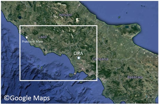
Figure 1.
The computational domain considered, including parts of Campania and Lazio regions. The CIRA and Pratica di Mare locations are specified.
Figure 2 shows the distribution of the heights (m) of the 60 vertical levels of the model. The majority of them are positioned close to the soil, and seven levels are positioned in the LOON flight zone (between 15 and 20 km), which can be considered a sufficient number for the purposes of the present investigation.
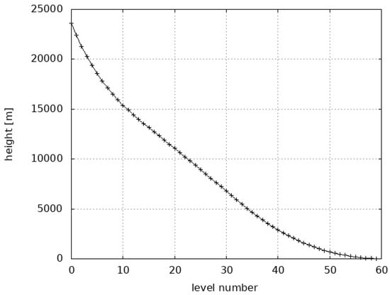
Figure 2.
Heights (m) of the 60 levels of the COSMO model. Seven are inside the LOON flight zone (15–20 km).
The capabilities of the COSMO model in terms of reproducing the main atmospheric variables over this area have been widely tested, in particular against data provided by the CIRA weather instrumentation, and the results of the model evaluation are presented in [23]. It was shown that the model is able to accurately reproduce the 2 m temperature, though it has difficulties in localizing intense rain events in this complex orography area. Wind values were compared with data provided by the wind profiler installed at CIRA (owned by ARPAC—the Environmental Protection Agency of Campania), revealing that they are generally well reproduced, especially at between 4 and 6 km, suggesting great potential of the model to support wind forecasts. Temperature profiles provided by the radio sounding performed at Pratica di Mare airport were compared with the model values in the grid-point closest to this location, highlighting a good reproduction of temperature and dew point profiles (maximum bias of 1 °C). In the present work, a detailed evaluation of the wind profiles provided by the model has been performed against radio sounding data in Pratica di Mare (Section 5.1), being the only stratospheric observational values available over the domain considered. Specifically, radiosonde data archived at the University of Wyoming (https://weather.uwyo.edu/, accessed on 17 June 2022) have been used, as they represent a frequently adopted reference for model assessments [24]. Evaluation was conducted considering daily data over the period 1 May 2021–30 April 2022. For each day, data at 00 and 12 UTC were considered, according with sounding data availability.
5. Results
5.1. Model Evaluation
In order to quantify model performances, standard indices for performance evaluation have been calculated: mean bias (BIAS) and root-mean-square error (RMSE), defined as:
where Si and Oi are, respectively, the simulated and observed values at the i-th level; N is the total number of vertical levels considered. Further, the time correlation between simulated and observed values (CORR) and the ratio between model and observation standard deviations (STD_RATIO) were evaluated. All the indicators were obtained considering the COSMO values (for each level) interpolated to the closest heights where radio sounding data are available.
Figure 3 shows the time series of the daily wind speed BIAS (left) and wind direction BIAS (right) over the period 1 May 2021–30 April 2022 for each day at 00 UTC and 12 UTC. On the horizontal axis, step 1 refers to 1 May 2021 h 00, step 2 refers to 1 May 2021 h 12 and so on, until step 730, which refers to 30 April 2022 h 12. These plots reveal good behavior of the model in reproducing the wind speed, the bias generally being between −1.5 and 1.5 m/s and never exceeding values ±3 m/s. Wind directions are quite well reproduced too, but there are some days (e.g., 7 June 2021 h 00) in which the bias is excessively large. Table 1 shows the numerical values of the indicators considered for wind speed, obtained by averaging the daily values (at 00 and 12 UTC) over each month of the year considered. Daily maximum values of the BIAS for each month are also shown. The analysis of the table revealed that the model is able to simulate the average features of the wind profiles; in fact, the bias values are always lower than 0.3 m/s. Of course, compensation effects may take place, as revealed by the values of RMSE and daily maximum BIAS, which are generally lower than 3 m/s anyway. Model and observational values are well correlated. The numerical correlation is higher than 0.84, and SDT_RATIO values are generally close to 1. Table 2 shows the numerical values of the same indicators for wind direction, obtained by averaging the daily values (at 00 and 12 UTC) over each month of the period considered. Daily maximum values of the BIAS for each month are also reported. The model has quite good capabilities to simulate the wind direction, but it is evident that for some days in winter (but also in June) the model fails to simulate the direction. Winter biases could be connected with the polar vortex, which is a large cyclone able to produce intense winds. It forms in November, when the stratosphere over the North Pole starts to cool down. Typically, a polar vortex circulation is interrupted in March or April due to a temperature increase in the stratosphere, called a sudden stratospheric warming (SSW) event. The stratospheric polar vortex variability has effects on the tropospheric circulation and in particular on the winter weather, so it is clear that accurate predictions of extreme polar vortex states are important to improve forecasts in winter, including cold spells. Unfortunately, current dynamical models have some limitations, because they poorly capture low-frequency processes [25]. The analysis performed in the present work over the year running from May 2021 to April 2022 has highlighted that that for most of the cold season the polar vortex was stronger than normal, and that the model’s performance slightly worsens from November to January.
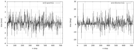
Figure 3.
Time series of the bias of wind speed (left) and wind direction (right) over the period 1 May 2021–30 April 2022.

Table 1.
Average values over the vertical profile of the mean monthly bias of wind speed (BIAS) (m/s), daily maximum bias (Max BIAS) (m/s), mean monthly root-mean-square error (RMSE) (m/s), mean monthly time correlation between simulated and observed values (CORR), mean monthly ratio between model and observational standard deviations (SDT_RATIO).
Table 2.
Average values over the vertical profile of the mean monthly bias of wind direction (BIAS) (deg), daily maximum bias (Max BIAS) (deg), mean monthly root-mean-square error (RMSE) (deg), mean monthly time correlation between simulated and observed values (CORR), mean monthly ratio between model and observational standard deviations (SDT_RATIO).
It is worth noting that part of the model error could be due to measurement uncertainties. In fact, under the push of horizontal winds, the radiosonde could move horizontally during the measurements, but data about the horizontal movements of the balloon are not available, so it is necessary to assume that the chosen grid point on the surface is always the same during the vertical measurements. In any case, the wind velocity evaluated by the model in an assigned grid point generally differs from the near points (on the same vertical level) by no more than 3%, so this source of uncertainty is limited.
In order to have more detailed information about model performance, vertical profiles were analyzed for selected days, namely, 2 July 2021, 2 October 2021, 2 January 2022 and 2 April 2022, which were chosen as representatives of the four climatological seasons (JJA, SON, DJF and MAM), for monitoring the model’s behavior under different weather situations. For each day, weather conditions in terms of ground temperature T and ground wind speed WS are provided. Figure 4 shows the vertical profiles provided by model data and radiosondes for the selected days. The heights considered range from 0 to 23 km, corresponding to the pressure range 1010–36 hPa. On 2 July 2021 h00 (sunny day, T = 24 °C, WS = 3.4 m/s), radio sounding data show a regular growth of wind speed values (with inversions at 5 and 8 km) from the ground up to 12 km. It reaches the value of 42 m/s; then it decreases until the value of 5 m/s at a height of 18 km. The model shows an excellent ability to reproduce the shape of the profile, and even the inversion at 8 km is captured. Moreover, wind values in the LOON zone are properly represented too. A similar profile can be observed at h 12, which is well reproduced by COSMO. On 2 October 2021 (thunderstorms, T = 21 °C, WS = 5.5 m/s) at h 00 and h 12, the general observational trend is well simulated by the model, especially up to 15 km. In the LOON zone, the wind speed is irregular, and the model is not able to capture the relative maximum and minimum values observed at specific heights, since it only reproduces the average decreasing trend. On 2 January 2022 (foggy day, T = 10 °C, WS = 2.7 m/s) at h 00 and h 12, the model well reproduces the inversions observed up to 15 km, but the maximum/minimum values in the LOON zone were not properly simulated. For 2 April 2022 (thunderstorms, T = 11 °C, WS = 8.9 m/s) at h 00, the observed profile up to 13.5 km was fairly reproduced, though larger values of wind speed above 38 m/s were underestimated. At h 12, the observed profile is highly irregular, but the model performs quite well in the LOON zone too, even if the low vertical resolution penalizes the accuracy. Table 3 shows the average values of performance indices for the selected days (h 00 and h 12). The mean biases averaged only on the points in the LOON zone (BIAS_LOON) were evaluated too, along with the corresponding biases after interpolation (BIAS_INTP; see below). Good agreement between model and observations was found in terms of BIAS, the values being less than 1 m/s. A high correlation is generally reported, and SDT_RATIO values are satisfactory too. In the LOON zone, the model suffers from higher biases, which is particularly evident for 2 July 2021. In order to increase the model accuracy in this zone, following the approach adopted in [2] for temperature profiles, a fifth order vertical interpolation of the wind speed model values in the LOON zone is proposed. Figure 5 shows the vertical profiles of wind speed in the LOON zone for the selected days provided by the radio sounding, the COSMO model and by the fifth order interpolation of the model data. As confirmed also by numerical values reported in Table 3, it is evident that the proposed interpolation allows an improvement of the representation of the vertical profile, with a bias reduction ranging between 10 and 25%.
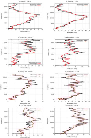
Figure 4.
Vertical profiles of wind speed for selected days (h 00 and h 12), provided by the radio sounding and by the COSMO model.
Table 3.
Average values over the vertical profile of the mean bias (BIAS) (m/s), root-mean-square error (RMSE) (m/s), time correlation between simulated and observed values (CORR), ratio between model and observational standard deviations (SDT_RATIO), mean bias in the LOON zone (BIAS_LOON) (m/s) and mean bias in the LOON zone after fifth order interpolation (BIAS_INTP) (m/s).
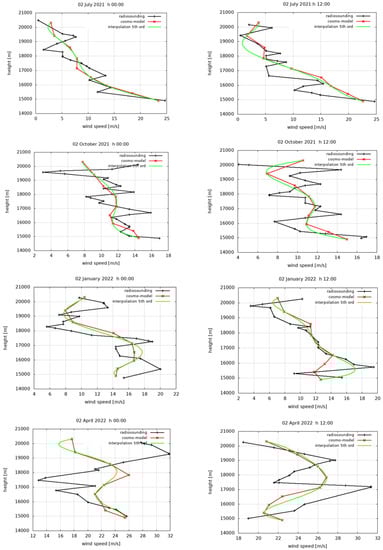
Figure 5.
Vertical profiles of wind speed in the LOON flight zone (15–20 km) for selected days provided by the radio sounding, COSMO model and fifth order interpolation of the model data.
5.2. Analysis of Time Series
Hourly time series of stratospheric wind speeds provided by COSMO for selected months have been extracted at Pratica di Mare at heights of 15.9 km (level 10) and 19.3 km (level 5). Figure 6 (left column) shows the time series for the months October 2021, November 2021 and April 2022. The time series were processed by using an FFT to produce a power spectrum of wind at regularly spaced bins, on order to measure the amounts of variability occurring in different frequency bands. The frequency resolution is 1/T0 = 1.54 × 10⁻³ (given that T0 is 648 h). Figure 6 (right column) shows the corresponding mean power spectra (log-log representation). In October 2021, a regular pattern in the time series can be observed, and three main peaks are visible in the power spectrum (f = 4.63 × 10⁻³, 7.71 × 10⁻³, 1.23 × 10⁻²), corresponding to periods of 216, 129 and 81 h respectively. In November 2021, three main peaks are visible too (f = 9.25 × 10⁻³, 1.54 × 10⁻², 1.85 × 10⁻²), corresponding to periods of 108, 65 and 54 h. Finally, in April 2022, only one peak is clearly visible (f = 2.7 × 10⁻²) corresponding to a period of 37 h. For all months, the spectra in the range of low frequencies tend to have a decreasing shape with superimposed noise. The distribution in the range of higher frequencies (>3 × 10⁻²) has been compared with the power law predicted by Kolmogorov for homogeneous isotropic turbulence (blue lines in the figures). According to the Kolmogorov theory [10], the turbulence velocity spectrum can be separated into frequency ranges, generally expressed as a turbulence source region (large scale), inertial subrange (intermediate scale) and dissipation region (small scale). The Kolmogorov law [26] predicts that if the constant and the energy loss rate of a turbulent fluid are constant, then the energy is controlled only by the scale of turbulence raised to the −5/3 power. From the figures, it is evident that at high frequencies, the wind power output spectrum displays a power law close to the Kolmogorov distribution. It is important to point out that the Fourier power spectrum is a second order statistic, which provides information on medium level fluctuations, so its slope is not sufficient to fully describe a scaling process, so additional investigations are needed to fully explore these mechanisms and develop a physical framework that can be incorporated into the study of turbulence.
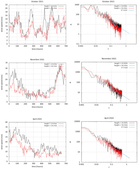
Figure 6.
(left column) Time series of stratospheric wind speeds for selected months extracted at Pratica di Mare location at heights 15.9 km (level 10) and 19.3 km (level 5); (right column) corresponding mean power spectra obtained by FFT.
6. Conclusions
In the last few decades there has been renewed interest in the commercial usage of the stratosphere, since there it is possible to use less expensive and higher resolution Earth monitoring services with respect to satellites, covering four times the areas of standard aircraft. With the horizontal motion of stratospheric balloons being associated with winds, the importance of accurate wind forecasts in this part of the atmosphere is evident. In this work, a review of wind prediction techniques for the stratosphere was provided, achieved by the most popular global models, such as ECMWF IFS, NCEP GFS and ICON. Then, the ability of the COSMO limited area model to reproduce the wind speed in the stratosphere was evaluated considering a model configuration at 1 km resolution. In fact, it is well known that very high resolutions are challenging in weather models for short- and medium-term forecasts. Considering the computational costs required, it is necessary to evaluate the forecast quality and to understand the model’s deficiencies.
Global simulations show that the simulated zonal-mean circulation in the troposphere is only moderately sensitive to the horizontal and vertical resolution adopted, whereas it appears that the simulation of the stratosphere can be much more sensitive to numerical resolution, even if quite fine grids are adopted. Changes with resolution are probably related to the skill of fine vertical resolution models in adequately representing the interaction of the mean flow with a wide spectrum of vertically propagating gravity waves.
The COSMO model was configured for the specific area of southern Italy considered; model performances were evaluated in terms of wind profiles against one year of daily radio sounding data collected in Pratica di Mare. Good agreement was found in terms of average bias and correlations, but compensation effects were present, since the model was not able to capture maximum and minimum wind speed values in the LOON flight zone. Some improvements can be achieved by employing a fifth order vertical interpolation of the wind speed model values. The analysis of monthly time series revealed the presence of a scaling regime or power law correlation of the form f−β over a broad range of time scales, in the Fourier space. The exponent spectral β is close to the exact 5/3 Kolmogorov value for all the datasets. Of course, further evaluations of COSMO model are needed in other computational domains in Italy/Europe, where other radio sounding data are available for comparison.
Some of the challenging objectives to be achieved in the near future imply the development of subgrid-scale parametrization of nonhomogeneous, anisotropic, non-Kolmogorov, shear stratified, stratospheric turbulence and stratospheric aerosols, to be included in the next generation of mesoscale numerical weather prediction models for the lower stratosphere, to enable the forecasting of, e.g., nonlinear inertia-gravity waves that generate layers of clear air turbulence. In fact, gravity waves are recognized to influence the response to the variability of the large-scale stratospheric circulation, so their parameterization is a source of uncertainty in stratospheric predictions. Finally, since the COSMO consortium has started the migration from the COSMO-LM to the ICON-LAM as the future operational model, ICON-LAM is being calibrated at CIRA on the same geographical domain in southern Italy, and the model’s performances in the stratosphere will be evaluated in a future work.
Funding
This research received no external funding.
Data Availability Statement
Data stored at CIRA supercomputing center and available on request.
Acknowledgments
The author acknowledges Alessandra Zollo (CIRA) for the helpful suggestions provided.
Conflicts of Interest
The author declares no conflict of interest.
References
- Mahalov, A.; Moustaoui, M.; Nichols, B. Characterization of Stratospheric Clear Air Turbulence for Air Force Platforms. In Proceedings of the HPCMP Users Group Conference (HPCMP-UGC’06), Denver, CO, USA, 26–29 June 2006; pp. 288–295. [Google Scholar] [CrossRef]
- Polichtchouk, I.; Diamantakis, M.; Vána, F. Quintic vertical interpolation improves forecasts of the stratosphere. ECMWF Newsletter 2020, 163, 23–26. [Google Scholar] [CrossRef]
- Schmidt, H.; Brasseur, G.P.; Charron, M.; Manzini, E.; Giorgetta, M.A.; Diehl, T.; Fomichev, V.I.; Kinnison, D.; Marsh, D.; Walters, S. The HAMMONIA chemistry climate model: Sensitivity of the mesopause region to the 11-year solar cycle and CO2 doubling. J. Clim. 2006, 19, 3903–3931. [Google Scholar] [CrossRef]
- Richter, J.H.; Sassi, F.; Garcia, R.R.; Matthes, K.; Fischer, C.A. Dynamics of the middle atmosphere as simulated by the Whole Atmosphere Community Climate Model, version 3 (WACCM3). J. Geophys. Res. Atmos. 2008, 113, D08101. [Google Scholar] [CrossRef]
- Watanabe, S.; Kawatani, Y.; Tomikawa, Y.; Miyazaki, K.; Takahashi, M.; Sato, K. General aspects of a T213L256 middle atmosphere general circulation model. J. Geophys. Res. 2008, 113, D12110. [Google Scholar] [CrossRef]
- Hamilton, K. Numerical Resolution and Modeling of the Global Atmospheric Circulation: A Review of Our Current Understanding and Outstanding Issues. In High Resolution Numerical Modelling of the Atmosphere and Ocean; Hamilton, K., Ohfuchi, W., Eds.; Springer: New York, NY, USA, 2008. [Google Scholar] [CrossRef]
- Brasefield, C.J. Winds and temperatures in the lower stratosphere. J. Meteorol. 1950, 7, 66–69. [Google Scholar] [CrossRef]
- Hersbach, H.; Bell, B.; Berrisford, P.; Hirahara, S.; Horányi, A.; Muñoz-Sabater, J.; Nicolas, J.; Peubey, C.; Radu, R.; Schepers, D.; et al. The ERA5 global reanalysis. Q. J. R. Meteorol. Soc. 2020, 146, 1999–2049. [Google Scholar] [CrossRef]
- Modica, G.D.; Nehrkorn, T.; Myers, T. An investigation of stratospheric winds in support of the high-altitude airship. In Proceedings of the 13th Conference on Aviation Range and Aerospace Meteorology, AMS, New Orleans, LA, USA, 21–24 January 2008. [Google Scholar]
- Kolmogorov, A.N. Local Structure of Turbulence in an Incompressible Fluid at Very High Reynolds Number. Dokl. Akad. Nauk SSSR 1941, 30, 299–303. [Google Scholar] [CrossRef]
- Hortal, M. The development and testing of a new two-time-level semi-Lagrangian scheme (SETTLS) in the ECMWF forecast model. Q. J. R. Meteorol. Soc. 2002, 128, 1671–1687. [Google Scholar] [CrossRef]
- Sleigh, M.; Browne, P.; Burrows, C.; Leutbecher, M.; Haiden, T.; Richardson, D. IFS upgrade greatly improves forecasts in the stratosphere. ECMWF Newsletter 2020, 164, 18–23. [Google Scholar] [CrossRef]
- Candido, S.; Singh, A.; Delle Monache, L. Improving Wind Forecasts in the Lower Stratosphere by Distilling an Analog Ensemble into a Deep Neural Network. Geophys. Res. Lett. 2020, 47, e2020GL089098. [Google Scholar] [CrossRef]
- Panziera, L.; Germann, U.; Gabella, M.; Mandapaka, P.V. NORA nowcasting of orographic rainfall by means of analogues. Q. J. R. Meteorol. Soc. 2011, 137, 2106–2123. [Google Scholar] [CrossRef]
- Mnih, V.; Kavukcuoglu, K.; Silver, D.; Rusu, A.; Veness, J.; Bellemare, M.G.; Graves, A.; Riedmiller, M.; Fidjeland, A.K.; Ostrovski, G.; et al. Human-level control through deep reinforcement learning. Nature 2015, 518, 529. [Google Scholar] [CrossRef] [PubMed]
- Zängl, G.; Reinert, D.; Rípodas, P.; Baldauf, M. The ICON (icosahedral non-hydrostatic) modelling framework of DWD and MPI-M: Description of the non-hydrostatic dynamical core. Q. J. R. Meteorol. Soc. 2015, 141, 563–579. [Google Scholar] [CrossRef]
- Borchert, S.; Zhou, G.; Baldauf, M.; Schmidt, H.; Zängl, G.; Reinert, D. The upper-atmosphere extension of the ICON general circulation model (version: Ua-icon-1.0). Geosci. Model Dev. 2019, 12, 3541–3569. [Google Scholar] [CrossRef]
- Dawkins, E.C.M.; Feofilov, A.; Rezac, L.; Kutepov, A.A.; Janches, D.; Höffner, J.; Chu, X.; Lu, X.; Mlynczak, M.G.; Russell, J. Validation of SABER v2.0 operational temperature data with ground-based lidars in the mesosphere-lower thermosphere region (75–105 km). J. Geophys. Res. Atmos. 2018, 123, 9916–9934. [Google Scholar] [CrossRef]
- Hindley, N.P.; Wright, C.J.; Gadian, A.M.; Hoffmann, L.; Hughes, J.K.; Jackson, D.R.; King, J.C.; Mitchell, N.J.; Moffat-Griffin, T.; Moss, A.C.; et al. Stratospheric gravity waves over the mountainous island of South Georgia: Testing a high-resolution dynamical model with 3-D satellite observations and radiosondes. Atmos. Chem. Phys. 2021, 21, 7695–7722. [Google Scholar] [CrossRef]
- Steppeler, J.; Doms, G.; Bitzer, H.W.; Gassmann, A.; Damrath, U.; Gregoric, G. Meso-gamma scale forecasts using the nonhydrostatic model LM. Theor. Appl. Clim. 2003, 82, 75–96. [Google Scholar] [CrossRef]
- Doms, G.A. Description of the Nonhydrostatic Regional COSMO Model, Part I: Dynamics and Numerics; Technical Report; DeutscherWetterdienst: Offenbach, Germany, 2002.
- Lynch, P.; Huang, X.Y. Initialization of the HIRLAM model using a digital filter. Mon. Weather Rev. 1992, 120, 1019–1034. [Google Scholar] [CrossRef]
- Bucchignani, E.; Mercogliano, P. Performance evaluation of high-resolution simulations with COSMO over South-Italy. Atmosphere 2021, 12, 45. [Google Scholar] [CrossRef]
- Yang, J.; Duan, S.B.; Zhang, X.; Wu, P.; Huang, C.; Leng, P.; Gao, M. Evaluation of Seven Atmospheric Profiles from Reanalysis and Satellite-Derived Products: Implication for Single-Channel Land Surface Temperature Retrieval. Remote Sens. 2020, 12, 791. [Google Scholar] [CrossRef]
- Kretschmer, M.; Runge, J.; Coumou, D. Early prediction of extreme stratospheric polar vortex states based on causal precursors: Prediction of extreme vortex states. Geophys. Res. Lett. 2017, 44, 8592–8600. [Google Scholar] [CrossRef]
- Stull, R. An Introduction to Boundary Layer Meteorology; Kluwer Academic Publishers: Dordrecht, The Netherlands, 1988; 666p. [Google Scholar]
Publisher’s Note: MDPI stays neutral with regard to jurisdictional claims in published maps and institutional affiliations. |
© 2022 by the author. Licensee MDPI, Basel, Switzerland. This article is an open access article distributed under the terms and conditions of the Creative Commons Attribution (CC BY) license (https://creativecommons.org/licenses/by/4.0/).