Scaling Up: Molecular to Meteorological via Symmetry Breaking and Statistical Multifractality

Abstract

The path from molecular to meteorological scales is traced and reviewed, beginning with the persistence of molecular velocity after collision induces symmetry breaking, from continuous translational to scale invariant, associated with the emergence of hydrodynamic behaviour in a Maxwellian (randomised) population undergoing an anisotropic flux. An empirically based formulation of entropy and Gibbs free energy is proposed and tested with observations of temperature, wind speed and ozone. These theoretical behaviours are then succeeded upscale by key results of statistical multifractal analysis of airborne observations on horizontal scales from 40 m to an Earth radius, and on vertical scales from the surface to 13 km. Radiative, photochemical and dynamical processes are then examined, with the intermittency of temperature implying significant consequences. Implications for vertical scaling of the horizontal wind are examined via the thermal wind and barometric equations. Experimental and observational tests are suggested for free running general circulation models, with the possibility of addressing the cold bias they still exhibit. The causal sequence underlying atmospheric turbulence is proposed.

1. Introduction

The central importance of symmetry for the conservation laws of physics was pointed out by Noether [1]; there was no scale specified for the operation of the principle. The possibility of breaking such symmetries in a solid-state physics context was stated by Landau [2]. Anderson [3] extended the approach into mathematical forms that proved eventually to be ground-breaking in condensed matter and particle physics [4]. Systems with continuous symmetries need not have conservation laws; Hamiltonian treatments with Lagrangians, such as chaotic attractors in phase space, are undermined by dissipation, a situation characteristic of the atmosphere. Although mathematically dissipation in chaos theory is represented by shrinking of the phase space, such a process is irrelevant in the atmosphere, where multiplicative interaction on all scales between absorption of solar photons and emission of infrared ones to the coldness of space is operative. The possibility of the continuous translational symmetry, shown by Maxwellian samples of gas molecules treated as hard spheres, being applicable to air is confounded—broken—by the persistence of velocity after collision [5] and the molecular dynamics result of the emergence of fluid flow under anisotropic flux [6], a ubiquitous atmospheric condition. These considerations were brought into sharp relief by the application of the theory of statistical multifractality to atmospheric observations of sufficient quality by Schertzer and Lovejoy [7,8,9] and later with a molecular emphasis by Tuck and co-authors [10,11,12,13,14]. The implications of these analyses are dealt with in the succeeding sections of this paper.

Arguments are provided as to how the scaling-based Gibbs free energy provides the work needed to drive the atmospheric circulation, having been deduced from the molecular collisions involved in producing vorticity on short time and space scales by a nonlinear process that shows how temperature remains defined operationally and acts as the integrator in a fluctuation-dissipation theorem, being influenced differently by gravity than the other variables. The observational data used to successfully test the scaling theory and the values of its exponents were obtained by the NASA ER-2 (Lockheed, Burbank, CA, USA) and DC-8 (McDonnell Douglas, St. Louis, MO, USA) aircraft during polar ozone missions, with midlatitude and tropical flights also included; the NASA WB57F (English Electric, Preston, UK; General Dynamics, Fort Worth, TX, USA) was used in the northern hemisphere tropics and midlatitudes, while the GPS dropsonde observations were made from the NOAA G4-SP (Gulfstream, Savannah, GA, USA) during the Winter Storms projects in January–March of 2004, 2005 and 2006 above the Pacific Ocean from (15°–60° N, 128°–172° W).

We shall see that correlation of the three scaling exponents H, C₁ and α with conventional variables provides insight into the operation of some physical processes, such as temperature, sources and sinks, and jet streams.

The procedure will be to review the work undertaken since 1998 via a selection of key diagrams, accessing more detailed formulations and discussions by references.

2. Microscopic and Macroscopic Processes

The coupling of molecular and meteorological processes is shown schematically in Figure 1. It is through the central variable of temperature.

2.1. Persistence of Molecular Velocity after Collision

The persistence of molecular velocity after collision [5] breaks the continuous translational symmetry (randomness) assumed in speed and direction that underlies the Maxwell–Boltzmann probability distribution function (PDF) and hence Lorentzian and Doppler spectral line shapes used in radiative transfer in the atmosphere. Einstein–Smoluchowski diffusion is also negated in the atmosphere and with it the definition of temperature used in laboratories. Maxwell–Boltzmann PDFs have continuous translational symmetry, which is broken by the persistence of velocity after collision.

$${\mathsf{\varpi }}_{12}=\frac{1}{2}{m}_{{}_1}+\frac{1}{2}{(m_1)}^2{(m_2)}^{-1/2}\ln [(\sqrt{m_2}+1)/{(m_1)}^{1/2}]$$

(1)

The persistence ratio ϖ₁₂ is the ratio of the mean velocity after collision to that before collision between molecules of masses m₁ and m₂. If m₁ = m₂ then ϖ₁₂ = 0.406, but in general for m₁ ≠ m₂ the heavier molecule will be slowed less than the lighter one.

This breaking of continuous translational symmetry will be discussed further later in the light of observational analyses, but it immediately leads to the interpretation of molecular dynamics calculations that showed the emergence of hydrodynamic behaviour in a population of randomised molecules subject to an anisotropic molecular flux [6]. This phenomenon is shown in Figure 2. Here ‘molecules’ are represented as hard spheres (‘billiard balls’); ring currents—vortices—emerged on very short time and space scales.

It is suggested from the outset that a vorticity approach be adopted from this smallest, molecular scale. Let ω be the vorticity of the field of molecular velocity v [14]:

$$\omega =\nabla \times v$$

(2)

This enables calculation of twice the enstrophy directly by taking the curl of the molecular velocity field:

$$\langle \omega ·{\omega }^{″}\rangle =-\nabla \langle v· v^{\prime }\rangle$$

(3)

Because enstrophy propagates downscale, in 2D theory at least, it may be less suited to describing the behaviour of energy deposited on the smallest scales, that of photons and molecules as it is in the atmosphere. The vorticity correlation function can lead to the vorticity form of the Navier–Stokes equation; see Section 3.3 of [15]. Nevertheless, the vorticity of ‘air’ in a molecular dynamical calculation is obtainable by:

ω = ∇ × v(p,q)

(4)

where p is molecular momentum and q is molecular position. They are necessitated by the non-spherical symmetries of real molecules and the omnipresent anisotropies of gravity, planetary rotation and the solar beam. The nth moment of the molecular speed is [14,15,16]:

$$\overline{v^n}=\frac{2}{\sqrt[2]{\pi }}{\left(\frac{2T}{m}\right)}^{\frac{n}{2}}\mathsf{\Gamma }\left(\frac{n+3}{2}\right)$$

(5)

This equation permits n to be used in calculating moments in the course of statistical multifractal analysis of molecular dynamics calculations.

2.2. Emergence of Fluid Flow from a Molecular Population

Figure 2 illustrates the discovery of this phenomenon by Alder and Wainwright [6]. It was appealed to in a meteorological context as the result of an unexpected observational correlation between the ozone photodissociation rate and the intermittency of temperature [14], about which more later. Physically, the mechanism consists of the faster molecules pushing up higher number density ahead of themselves, leaving lower number densities in their rear. The resulting number density gradient results in a flux of the more numerous, nearly average molecules that produces the ring current. The numerous, near average molecules exchange collisional energy easily, and in so doing maintain an operational temperature, which is not, however, described by a Boltzmann PDF. Note that the interactions are non-linear and result in the vorticity structure being self-sustaining, offering the ability to propagate upscale.

Extant statistical multifractal analyses expected temperature to scale like a passive scalar (a tracer), but the earliest such treatments of NASA ER-2 data in the lower stratosphere at 17–20 km altitude showed that temperature scaled differently than known tracers [10,11,12], at least under rescaled range analysis. With the availability of high-resolution GPS dropsonde data from the NOAA Gulfstream G4-SP, it became clear from statistical multifractal analyses that temperature was affected differently by gravity than other variables [15,17,18,19]. The scaling of temperature spans the range from micro (molecular) through meso (nanometres to micrometres) to macro (>micrometres). That accounts for temperature acting as a kind of integrator in the way that other variables do not.

A further implication of the Alder–Wainwright mechanism is in the basis of the fluctuation–dissipation theorem as embodied in the Langevin equation. Langevin treated the mean as organised behaviour and fluctuations as dissipation. The Alder–Wainwright mechanism implies the reverse, that the hydrodynamic fluctuation carried by the fastest molecules represents emergent organisation and the mean represented by the near average molecules represents dissipation that defines an effective temperature. Further discussion may be found in chapter Sections 3.1–3.3, 5.2 and 8.1 of [15].

We cannot expect to view atmospheric vorticity in two dimensions and remain quantitative, because the dimensionality of atmospheric flow is 2 + H(s), [8,9,15] where H(s) is the vertical scaling exponent of the horizontal wind, s. The vorticity form of the Navier–Stokes equation is:

$$\frac{D\mathit{\omega }}{Dt}=(\mathit{\omega }·\nabla )u+\kappa {\nabla }^2\mathit{\omega }$$

(6)

where κ is kinematic viscosity. The first term on the right says that vorticity, ω, advects itself: nonlinearity is inherent. This term alone is responsible for much of the complexity and difficulty associated with understanding, describing and computing atmospheric flow. ω is defined by Equations (2) and (3) and using (3) we can relate the autocorrelation function for vorticity, A(t), to the enstrophy ε:

$$\epsilon =\frac{{\left|\omega \right|}^2}{2}=A(t)$$

(7)

Enstrophy is governed by:

$$\frac{D}{Dt}\left(\frac{{\left|\omega \right|}^2}{2}\right)={\omega }_i{\omega }_{j}St{r}_{ij}-\kappa {\left|\nabla \times \omega \right|}^2+\nabla \left[\kappa \omega \times (\nabla \times \omega )\right]$$

(8)

where Str_ij is the straining rate on a fluid element.

Equation (8) expresses the generation of vorticity by stretching, or its destruction by compression, via the first term, balanced by viscous dissipation in the second term. The third term is the divergence, often assumed to be locally zero; this cannot be strictly true, for example, if ozone photodissociation is leading to the generation of vorticity. Considering the theoretical case of 2D turbulence, there are reverse cascades of energy and enstrophy, upscale for the former and downscale for the latter. If photon energy is directly converted to vorticity as implied by the Alder–Wainwright mechanism, it would imply energy transfer upscale from the smallest, molecular, ones in the range of 10–100 nanometres at tropospheric temperatures and pressures. However, the point is moot because the scale invariant structure of the fluctuating abundances of the absorbers and emitters of radiation, including ozone, carbon dioxide, methane, nitrous oxide, halocarbons, aerosols and water in all its phases, means that energy is input and lost to air on all scales, eliminating the possibility of conservative energy or enstrophy cascades either upscale or downscale. The observed scale invariant 23/9 dimensionality of air also eliminates 2D theories from relevance.

3. Statistical Multifractality

The variability in air is defined by three multifractal scaling exponents, which have been evaluated from observations of adequate quality [20,21,22,23]. The mathematical structure underlying the definition of H, C₁ and α may be found in these references; the notation is that in [21,22].

Table 1. Equivalence between statistical thermodynamic and scaling variables.

Variable	Statistical Thermodynamics	Scaling Equivalent
Temperature	T	1/qkBoltzmann
Partition function	f	e−K(q)
Energy	E	γ
Entropy	−S(E)	c(γ)
Gibbs free energy	−G	K(q)/q

shows equivalences between the variables of equilibrium statistical thermodynamics and the scaling variables from statistical multifractal analysis as applied to open, non-equilibrium systems, which the atmosphere is. The equivalences in Table 1 result from mappings [20] via Legendre transforms; they are not merely formal similarities and lead to the thermodynamic form of multifractality [22].

The variables are obtained as follows. q defines the qth order structure function of the observed quantity. The scaling exponent K(q) is derived from the slope of a log–log plot of the signal fluctuations versus its range, and H is obtained from:

$$H=H\left(q\right)+K\left(q\right)/q$$

(9)

and examination of energy E in terms of a scale ratio produces an expression for the fractal co-dimension c(γ). C₁ is the co-dimension of the mean, characterising the intensity of the intermittency. The Lévy exponent α characterises the generator of the intermittency which is the logarithm of the turbulent flux; for a real system, its value may not be confined to the theoretical range.

In practice here we find H = 0.56, C₁ = 0.05 and α = 1.60. The theoretical ranges are 0 < H < 1; 0 < C₁ < 1 and 0 < α < 2. A Gaussian has H = 0.50, C₁ = 0 and α = 2. See [15,21,22] for further discussion, and below for analysis of observations. The actual values of the three scaling exponents for wind, temperature, ozone and other molecules may provide information about the variables and how they interact.

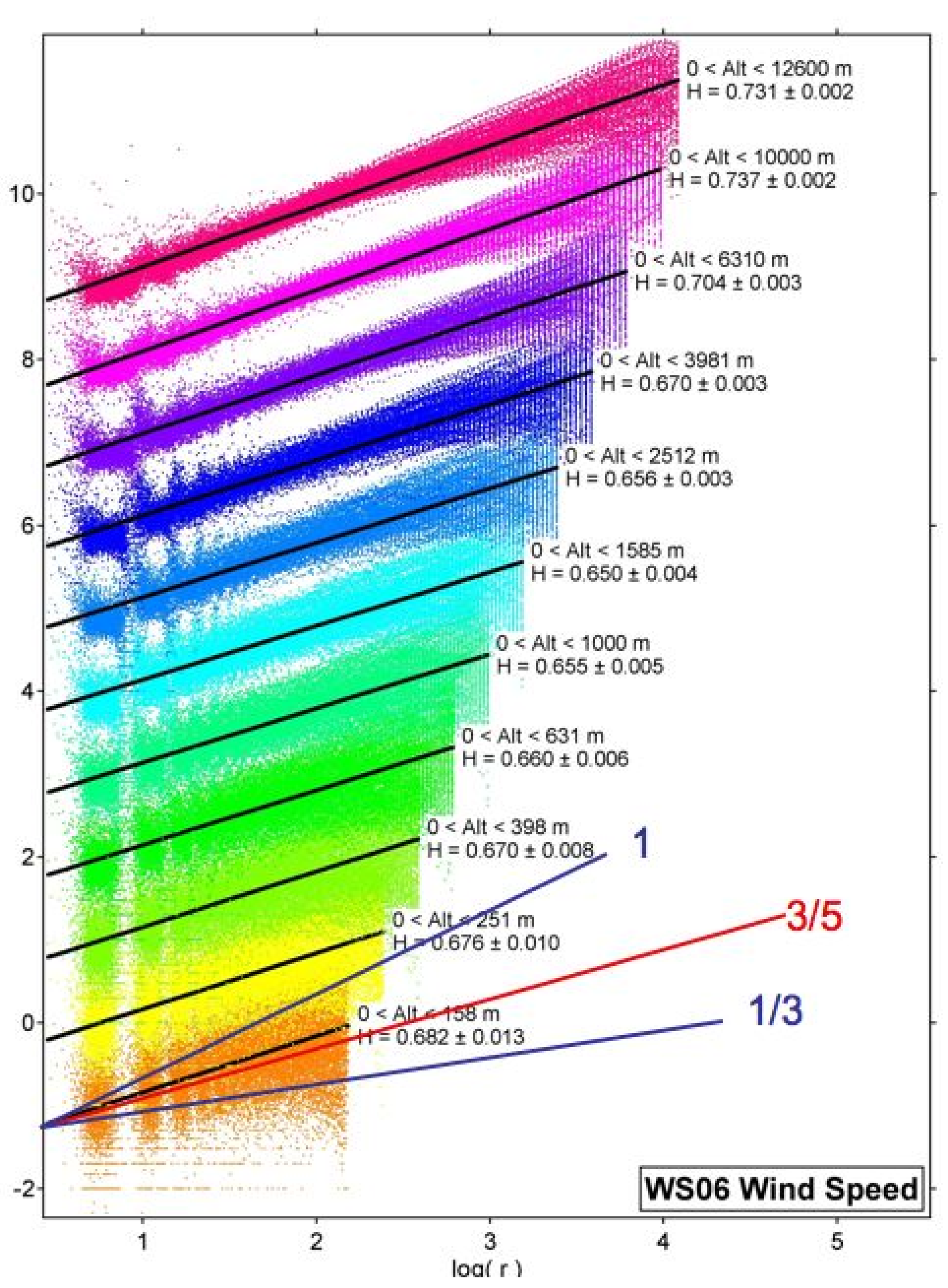
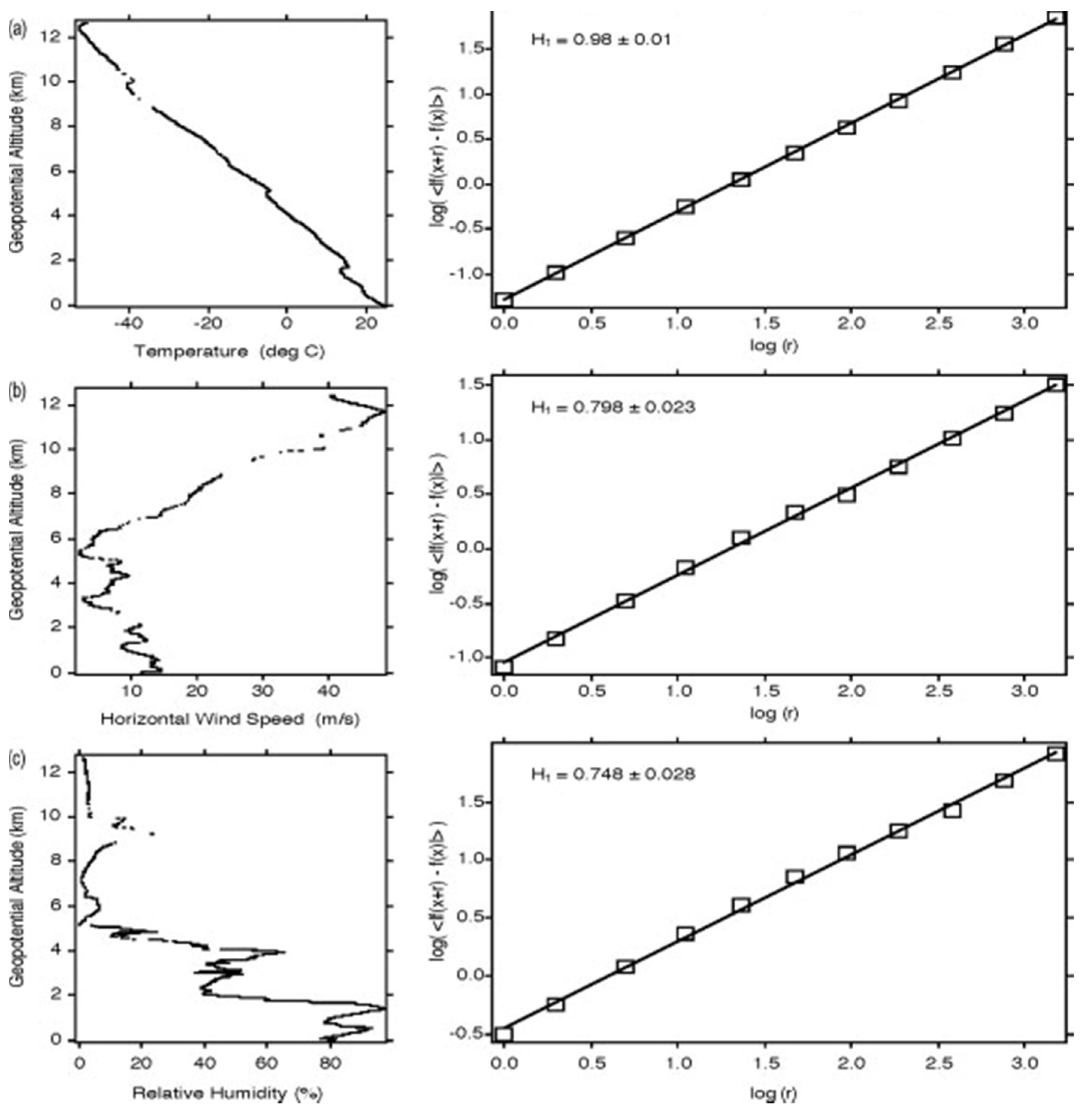
3.1. Vertical Scaling: Horizontal Wind, Temperature and Humidity

The vertical scaling of the horizontal wind, temperature and humidity was examined by statistical multifractal analysis of GPS dropsonde observations from the January–March NOAA Winter Storms missions of 2004, 2005 and 2006 [17,18,19,24,25,26]. The flight tracks were over the eastern Pacific Ocean of the Northern Hemisphere, from 15° to 60° N and 13 km altitude to the surface. Figure 3 summarises the 2006 data [19].

If the vertical scaling of temperature is calculated via spectral analysis, assuming for the purpose that intermittency is negligible, the value of H is approximately 5/4 while H for wind speed and relative humidity remains unchanged from the values in Figure 4b,c, respectively. The different scaling for temperature has been attributed to the effect of gravity on air density, upon which it acts directly, unlike wind speed and relative humidity [26]. It will be seen later that the effects of scaling in jet streams are also significant.

The dropsonde results are also apparent in stability analyses of all drops treated fractally [18]. The results were valid for dry adiabatic, dynamic (Richardson number) and moist adiabatic approaches. The correlation co-dimensions were respectively 0.36, 0.22 and 0.15, a demonstration of the importance of wind shear and moisture compared to a static dry adiabatic analysis. The corresponding fractal dimensions of the Cantoresque set are 0.64, 0.78 and 0.85.

In Figure 5, for one descent at 500 and 50 m resolutions, a broadly unstable lower troposphere and stable upper troposphere is seen, whereas at 15 m there are embedded unstable layers within stable layers at all scales, forming a ‘Russian doll’ structure characterised by a fractal dimension of 0.65. There are no unstable layers below about 50 m vertical dimension. This sonde was one of a pair dropped simultaneously; the high correlation of the structures seen by the two sondes eliminates the possibility that the signal is generated by noise [18].

Composite variograms from all 246 useable dropsondes during the Winter Storms 2004 mission, involving 10 flights over a wide area of the eastern Pacific Ocean of the Northern Hemisphere [19], are shown in Figure 6. See [15,18,19] for further description and analysis.

The ‘horizontal’ scaling of the aircraft observations has been calculated separately for the NASA ER-2 and WB57F mainly in the lower stratosphere, and for the NOAA G4-SP and NASA DC-8 mainly in the upper troposphere [15]. We note that there is an element of vertical velocity in such flight segments [27], and that during their ‘vertical’ segments the results for temperature, wind speed and humidity for the scaling exponent H agreed within 10% with the dropsonde results in the previous section [15,19]. The missions concerned ranged from pole to pole [15,19,28] when the DC-8 is included.

Figure 7 shows the observations of the longest ER-2 flight available, just over an Earth radius long on 19890220. It was one of the few on Arctic missions AASE, AASE-II and SOLVE that was along rather than across the lower stratospheric polar night jet stream (SPNJ). There were none along the Antarctic SPNJ during AAOE and ASHOE-MAESA [15,28]. There was a greater incidence of more variable encounters with jet streams by the WB57F during WAM, ACCENT, pre-AVE and CRYSTAL-FACE and by the G4-SP during Winter Storms 2004–2006, with the subtropical jet stream (STJ) and the polar front jet stream (PFJ); see [29].

The presence of an element of vertical velocity in the response of an aeroplane to the air in ‘horizontal’ flight leads to a prediction that the value of the scaling exponent H under statistical multifractal analysis should be 23/9, (2 + H), see [27], and this indeed proves to be the case [15,21]. The average values of H for wind speed and temperature over all qualifying flight legs for all aeroplanes are in the range 0.51 < H < 0.62 with a standard deviation of ±0.01 and an average of 0.55 overall, corresponding to the predicted 5/9, which arises from 1/3 ÷ 3/5. The values for water, ozone and nitrous oxide are discussed below in Section 3.3, on scaling in molecular species.

3.2. Scaling in Jet Streams

Figure 8 shows the scaling exponent H for wind speed during ER-2 flight segments along the Arctic SPNJ and across it for the Antarctic SPNJ. The result that the along jet flight segment has the lowest value of H for wind speed suggests that this most highly anticorrelated value is caused by the speed shear being more effective at producing less organised, more random flow than is directional shear. The directional shear then probably accounts for the higher value in the across-jet direction, corresponding to stronger, more organised flow. The results are consistent with the shears in Figure 7c and are responsible for the exchange of air and its chemical content between the vortex and its surroundings [15,21,30].

Similar results, although less accurate, were seen by the WB57F [29] in the subtropical jet stream (STJ). The speed shear’s effectiveness at producing anticorrelation—on all scales—may be why clear air turbulence is frequently experienced by aeroplanes at jet stream entrances and exits.

When all values of H for wind speed and temperature are plotted against traditional measures of jet stream strength as measured from the aeroplane, a correlation is seen in Figure 9: the stronger the jet stream as observed from horizontal gradients, the higher the value of H. A similar result may be obtained in the vertical from the GPS dropsonde data discussed in the previous section. The vertical scaling exponent for the horizontal wind is positively correlated with both jet stream depth and jet stream wind maximum, as seen in Figure 10.

3.3. Molecular and Photochemical Effects

The intimate connection between molecular behaviour and temperature seen earlier necessitates further examination of the behaviour of temperature in terms of its PDF, intermittency and the correlation of the latter with the ozone photodissociation rate. The observations were taken in the lower stratosphere during Arctic summer (April–September) in 1997 (POLARIS) and Arctic winter (January–March) in 2000 (SOLVE). Figure 11 shows the highly non-Gaussian PDFs. These missions had measurements of the ozone photodissociation rate [31] and are discussed in [14,15] and in the next section.

The relation between temperature and molecular velocity is given by equations 3.1 and 5.1 of [15]:

$$T=\frac{m}{3k}\langle {\left(v-\langle v\rangle \right)}^2\rangle$$

(10)

Figure 12 shows the scaling exponent H for ozone, for all ER-2 polar ozone missions: AAOE, AASE, AASE-II, ASHOE-MAESA and SOLVE. The mean value of 0.47 is less than the passive scalar (tracer) value of 0.55 (5/9), a consistent result for all molecular species under conditions where they are known to have a sink operating. The sequences of points with values resulting in H for ozone in the range of 1/4 to 1/3 are in the polar vortices in the classic ‘ozone hole’ regime; the scaling is good in the presence of active photochemical loss [15,21,22,32]. The mean value of H for ozone is 0.47, reflecting ozone loss outside and inside the polar vortices in both hemispheres. Regarding water as a molecule, we can see that it too can have scaling exponent H less than the theoretical tracer value of 5/9 in Figure 13. Here the observations are for total water (vapour plus ice measured as vapour) [15,32,33,34]. The sink is the falling of ice crystals under gravity, a process also seen for reactive nitrogen, NO_y, in nitric acid–water particles large enough to sediment [15,35,36]. The ozone instrument [37] was the only one with data characteristics of sufficient signal-to-noise ratio and continuity to obtain the three scaling exponents, intermittency C₁ and Lévy exponent α, in addition to the more robust H. The calculation of intermittency requires a good signal-to-noise ratio, a very low incidence of data dropouts and the use of double precision in computation.

The assumption that molecules with a sink process operative display values of H less than the 5/9 expected theoretically of a tracer (passive scalar) can be verified by inspection of Figure 14. During the ASHOE-MAESA mission of 1994, the observations of nitrous oxide, N₂O, were good enough to provide an experimental test of the assumption, because N₂O is a known tracer in the lower stratosphere [38]. Tracers do scale with the value of H predicted by the generalised scale invariance theory of statistical multifractals. This result should provide a test and a diagnostic for global models of the general circulation that run chemical mechanisms, whether for weather and air quality forecasting or attempts at climate prediction.

The observed value of the scaling exponent H for observations of chlorine monoxide [40,41], the chain-carrying free radical of the ozone catalytic destruction cycle during the SOLVE mission in the Arctic January–March 2000, is shown in Figure 15. The progression of the ClO traces and the associated scaling is shown from late January to mid-March and shows values characteristic of production in the early phase and of a sink in the late phase. These changes were accompanied by values characteristic of an ozone sink in all three days, indicating ozone loss prior to 20000123. Those results are consistent with the scaling behaviour of NOy and its role in the processing of unreactive forms of chlorine into reactive ones by polar stratospheric clouds. A longer discussion with more figures can be found in Chapters 4.3 and 6.2 of [15]. Empirically the molecular species with H values greater than 5/9 are those with a source, usually in the free atmosphere arising from either photochemical production or conceivably by gravitational settling in crystals from above, which then evaporate. Those observations with H less than 5/9 are those with a chemical thermodynamically or photochemically favoured sink, resulting in the dilution of energy density. During AAOE and SOLVE it was observed that the scaling exponents H and α for ozone showed correlated changes in the vortex, whereas the intermittency C₁ stayed constant at about 0.05. All three exponents for wind speed and temperature were unchanged throughout the missions. Atmospheric chemistry is inherently nonlinear [12,13,14,15,26,32,42], set in an inherently nonlinear fluid medium [7,8,9,20,22,23].

A further aspect on chemical kinetics lies in the application of the law of mass action in air [13]. Because in most atmospheric volumes the reactant molecules do not have random access to the entire 3D volume on a relevant time scale, their existence in 23/9 space must be accounted for, a process which will result in the acceleration of reactant rates through the reduction of the dimensionality [13].

A diagrammatic summary of AAOE and AASE vertical and latitudinal profiles can be found in [43]. Comprehensive accounts of all the ER-2 and DC-8 missions can be found in the relevant special issues of Journal of Geophysical Research D-Atmospheres and Geophysical Research Letters: volumes 94(D9,14) and 17(4), respectively.

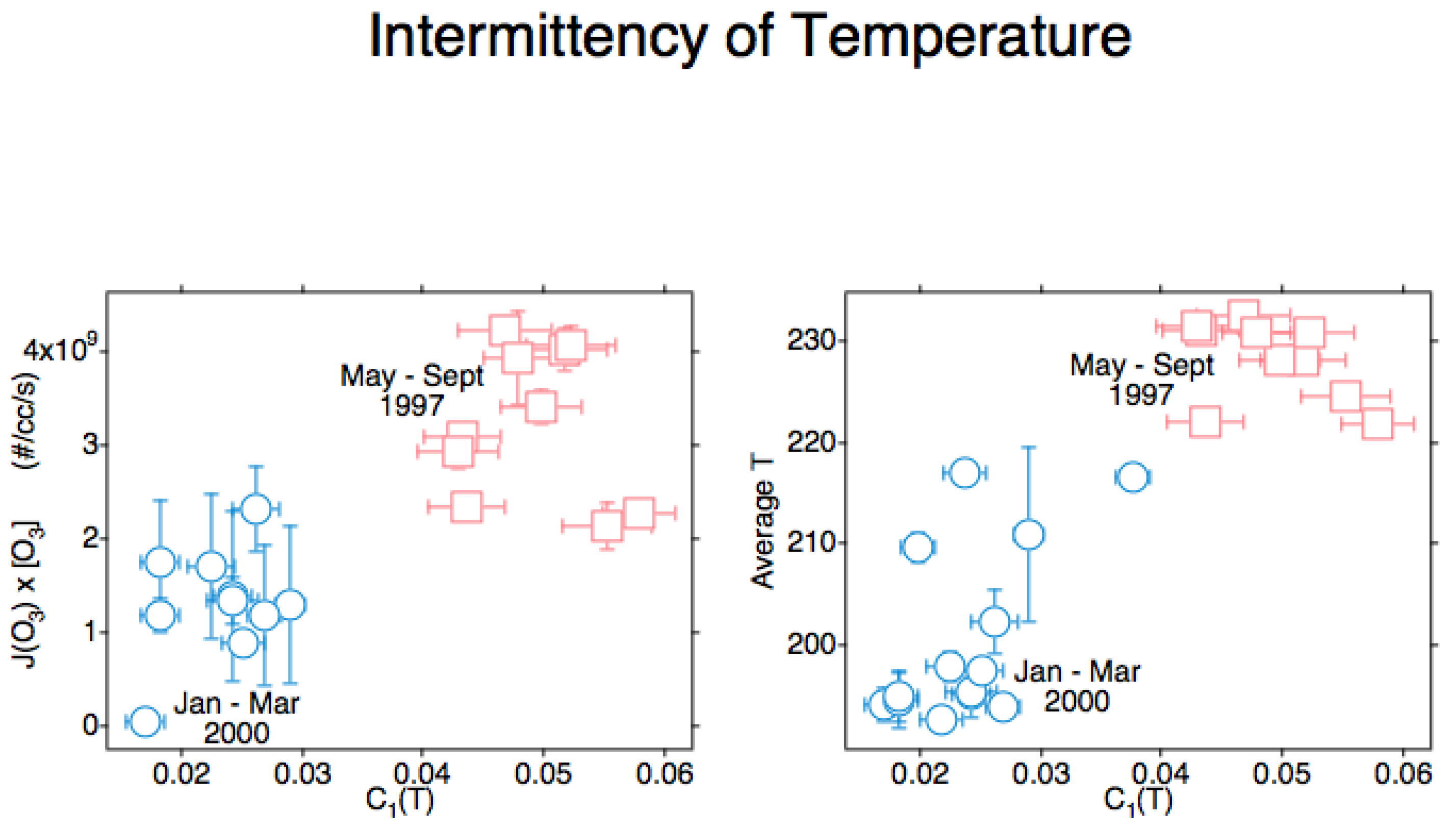
4. The Intermittency of Temperature and Its Correlation with Ozone Photodissociation Rate

An unexpected result from the measurement [31] of the ozone photodissociation rate, J[O₃], was positive correlation with the intermittency of temperature, C₁(T). That triggered a search for an explanation, with the causal attribution being the production of translationally hot O and O₂ photofragments recoiling into and acting in the vortices produced by the mechanisms seen in Figure 1 and justified in references [14,15,42]. The results from POLARIS in the Arctic summer of 1997 and from SOLVE in the Arctic winter of 2000 are displayed in Figure 16. C₁ (T) is positively correlated both with the ozone photodissociation rate and with temperature itself. By viewing Figure 11 in conjunction with Figure 16 and Figure 17, we can conclude that atmospheric temperature is not that of a gas in local thermodynamic equilibrium [26,32]. Account must be taken of molecular behaviour from the smallest scales up to the gravest; it will mean acting on the persistence of molecular velocity after collision [5] and its breaking of continuous translational symmetry of a thermalised gas via the Alder–Wainwright mechanism [6]. Further discussion occurs in Chapter 5.2 of reference [15] and in references [22,26,32,42]. Note that even when J[O₃] is zero, in the dark, the value of C₁(T) is not also zero, although it is lower than in sunlight.

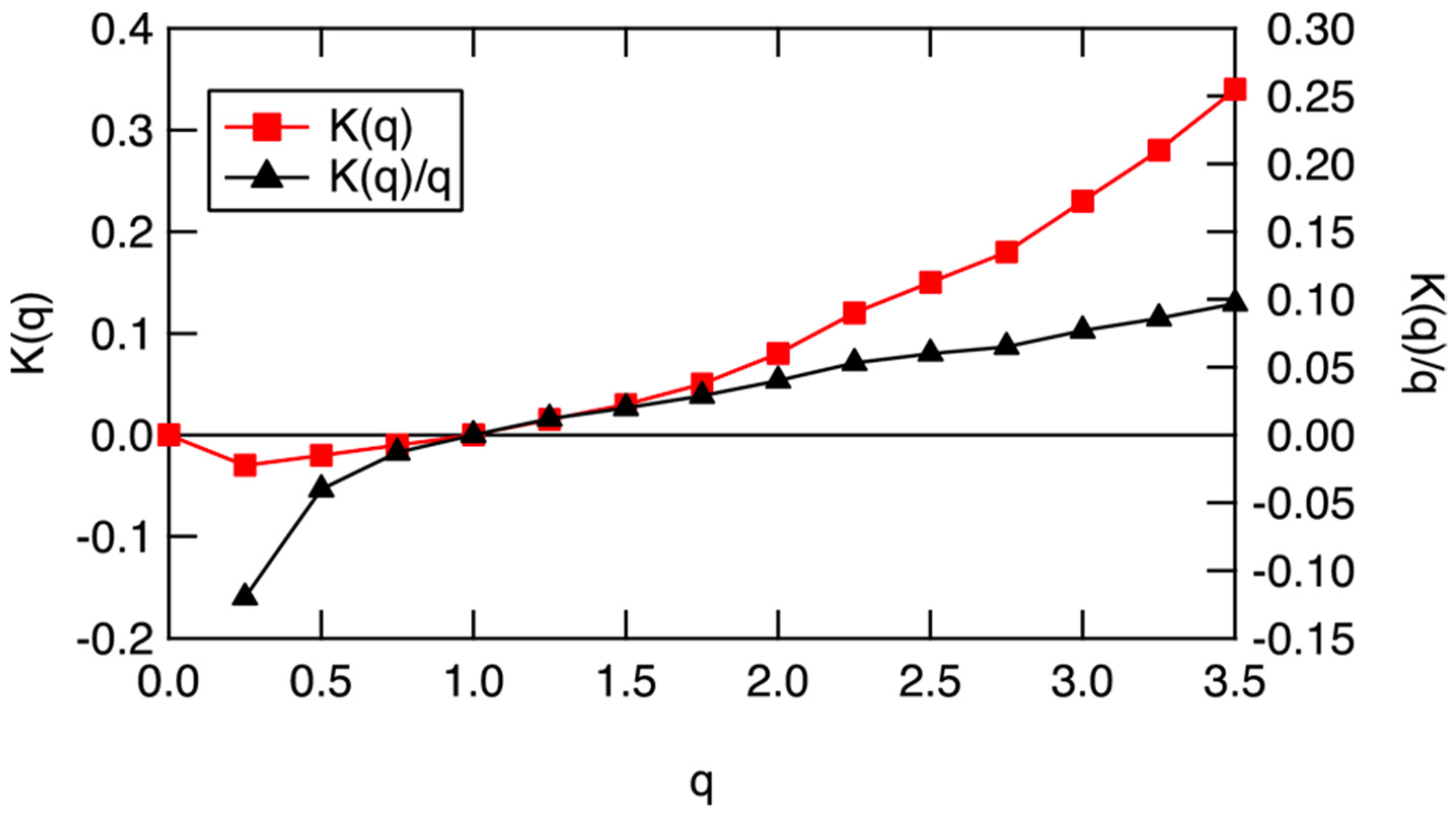
5. Scaling Based Entropy and Gibbs Free Energy

Given that the airborne in situ measurements of molecular species and photodissociation rates are unlikely to become routine, and are presently unattainable from satellite remote sounding, what can be done? Either locally by airborne methods or globally by satellites, it is not foreseeable to the extent necessary. One alternative approach is outlined in [22], where the thermodynamic form of statistical multifractality [20] is adapted [22] to produce Table 1. Those results enable diagnosis of steady states and system directionality from winds and temperatures, which are observed globally in a routine manner. The results in [22] vindicate the ‘bare’ cascade models of Schertzer and Lovejoy [9] and Lovejoy and Schertzer [20] by producing results from ‘dressed’ curves such as that in Figure 18, based on the data in Figure 17. Similar results were obtained for wind speed and ozone and are representative of all suitable 140 ER-2 flight segments between 1987 and 2000. Here, it is suggested that these diagnostics should prove applicable to global atmospheric models, particularly those dealing with air pollution and climate, wherein molecular species have to be simulated. Gibbs free energy does the work that drives the circulation to a different steady state under a perturbation, either on cooling or heating, after the entropic effects of dissipation have been accounted for.

What molecular behaviour should be expected in the nonequilibrium conditions displayed in Figure 17 and Figure 18? How will translationally hot and rotationally hot air molecules be manifest, whether observed by, for example, direct molecular beam sampling instruments or calculated by molecular dynamics methods? The red curve in Figure 19 is a hypothetical curve of the PDF of such molecular velocities, whereas the black curve represents an equilibrium Maxwell–Boltzmann state. The difference of the integrals beneath them via Equation (10) provides the Gibbs free energy. The atomic and molecular fragments from ozone photodissociation, which happens from the ultraviolet Hartley band through the Huggins, Chappuis and Wulf bands that stretch across the visible to the near infrared, can have up to an order of magnitude more energy than the average molecules.

The symmetry breaking causing non-Maxwellian velocity distributions, and hence non-equilibrium temperatures, will also limit theoretical and analytical techniques that impose a symmetry on the air that it does not possess; Fourier analysis for wave-based formalisms is a candidate for such limitations.

6. Aerosols and Scaling

The importance of aerosols for calculating the atmospheric state under global heating from fossil fuel combustion has been recognised as central for at least two decades [44], via their effect on radiative transfer and hence temperature. Recently, the COVID-19 pandemic virus has been observed to be of a size, having a diameter of about 80 nm dependent on water content, that enables it to be transported long distances by winds [45,46]. The dimensions of atmospheric aerosols span the scales from micro through meso to macro, and so are candidates for the application of scale invariant analysis [22,32,47].

Symmetry breaking is an important process in aerosols that have organic coatings, with division being asymmetric into a virally sized and a bacterially sized pair [48,49]. It is also important in the chemistry associated with microdroplets, in that reactions can be different for the different environments: the containing bulk medium, the interior of the particle and importantly, its surface where the free energy is concentrated in the form of surface tension [48,49,50,51].

From a climate heating prediction and action point of view, there are many uncertainties associated with aerosols in addition to those mentioned above and referenced in [42,44]. References [42,52] discuss them, and make it clear that geoengineering actions such as ‘solar radiation management’ are high risk options with uncertain outcomes.

One perspective that can be offered on the role of airborne transmission of bacteria and viruses is that atmospheric oxidant molecules, such as OH, HO₂, RO₂ and NO_x, will act as agents of evolution by natural selection ([32] and references therein), resulting in a coating that is more resistant to oxidative attack in air. It will vary with the fluctuating abundances of these molecules with geographic location and which, like all atmospheric constituents and variables, are influenced by scale invariant turbulent transfer. Aerosol sizes have power law distributions in the atmosphere, characteristic of scale invariance.

7. Models and Scaling

The effects of scaling analyses and the associated scale invariance and statistical multifractality provide a way of testing numerical models of the atmosphere that is an alternative to comparisons with observations localised geographically and temporally, such as zonal and monthly means [15,20,53,54,55,56,57]. Such models have, by necessity, to parameterise the lowest 8 decades of scale down from the gravest of the 15 that span the molecular mean free path to a great circle. The issues focused on here are tests, cold biases and maximum wind speeds. A start has been made in [55,56].

7.1. Scaling Issues and Tests for Models

An early attempt at comparing scaling analysis of an aircraft’s observations of temperature and wind speed revealed that the MM5 model inset into an ECMWF analysis for the flight on 19980411 did an inadequate job of simulating the mountain waves and the associated severe turbulence in the lee of the Wyoming Rocky Mountains [15,57]. Although the model simulation did scale, it was with different scaling exponents, as seen in Figures 4.13–4.15 and Table 4.2 of [15] and in [57]. More general results were obtained in [55], where global analyses from operational forecasting suites did scale in a manner similar to the predictions of the theories expounded in [20,23], but in better agreement along latitude circles than along meridians. We return to the disagreements seen with dropsonde data by [19] in Section 7.3 below. Detailed comparison with the structure of vortex species with potential vorticity fields and structure along ER-2 flight paths also revealed a lack of correlation on any but the coarsest scale using potential vorticity (PV) fields derived from operational assimilations [21,58,59]. That was not a surprise, given the resolution of the models: T63 in 1989 and T799 in 2010.

It is apparent that observations needed to implement scaling tests for numerical model simulations are in rather short supply. In particular, there are few meteorological research or operational aircraft flights with the necessary flight paths and quality. Commercial aviation data are available but, although they are invaluable for improving routine requirements such as wind speeds and temperatures by assimilation, they are not yet suitable for scaling analysis.

One observational experiment that could be performed [26,32] would be deployment of GPS dropsondes from a large constant-level balloon in the upper stratosphere. It would examine the hypothesis that the cold bias in free running models is caused by ozone photodissociation inducing a non-equilibrium state via persistence of molecular velocity breaking the continuous translational symmetry of equilibrated air, with associated induction of molecular scale vorticity via the Alder–Wainwright mechanism. Observation of J(O₃)[O₃] from the large balloon or even the dropsondes would add support.

7.2. Scaling and the Cold Bias in Models

There has been a persistent cold bias in free running numerical models of the global atmosphere, which has been confirmed recently by comparison of upper stratospheric analyses with observations from lidar temperature profilers [60]. Suggestions have been made based on scaling approaches that these cold biases may be the result of inadequate accounting for molecular effects [15,26,32,42] arising from results reported in [19]. The intermittency of temperature and its correlation with the ozone photodissociation rate evident in Figure 16 provided the clue to the non-equilibrium state of the air in the lower stratosphere, discussed at length in [15,32]. The posited cause is the recoil of translationally and rotationally ‘hot’ fragments from ozone photodissociation. Molecular effects causing departures from equilibrium will increase with altitude, as pressure quenching of ‘hot’ atoms and molecules, and the effect of gravity decrease [26,32]; the ozone photodissociation rate increases with height above the maximum in ozone density at 24–30 km. Those effects will have the largest influence on temperature in the upper stratosphere.

7.3. Scaling, Molecules and Maximum Observed Wind Speeds

The wind speeds that have been recorded and analysed in the atmosphere have maxima in locations such as the subtropical jet stream and the polar night stratospheric jet stream that exceed one quarter and even one half the speed of sound, particularly in the upper stratosphere [21,61]—for example 364 knots (180 ms⁻¹) at 47 km altitude above South Uist in December 1967—and also in more local phenomena such as hurricanes and tornadoes. These velocities of order 100 ms⁻¹ call into question the assumptions made in numerical models of the atmosphere in integrating the Navier–Stokes dynamical equations, the most significant of which is that the maximum fluid velocity should be much less than the average molecular velocity. Wind shears produce gradients of a steepness that are also beyond the capacity of current models to simulate accurately, particularly in the presence of intense turbulence [57].

The result that speed shear in the along jet direction is most effective at producing anticorrelation in jet streams, as shown in Figure 8 and discussed in Section 3.3, may account for the fact that turbulence in clear air is experienced by aircraft most frequently near jet stream entrances and exits, see Section 6.1.6 of [61].

8. Some Examples

Scaling analysis has been applied to ground based total ozone [62,63,64] and the incident solar flux [65], illustrating long memory in total (overhead column) ozone and the fact that incident solar radiation also shows scale invariance, with considerable intermittency. The reference list contains many papers in which statistical multifractals have been used to analyse a wide range of geophysical processes, most notably climate [20,23].

9. Why Turbulence?

This question, asked by Heisenberg three decades after his formulation of isotropic turbulence [66], had provoked earlier comment by fluid dynamicists Lamb and von Kármán and by theoretical physicist Feynman. Eady [67] argued that the turbulent transfer of heat was the fundamental driver of the atmospheric circulation, with such phenomena as jet streams, Hadley, Walker and Ferrel cells being secondary phenomena. This idea was examined more mathematically by Eady and Sawyer [68]. It is consistent with the view argued here and in [26,32] to the effect that energy is deposited in the air on the smallest scale—molecules and photons—and propagates upscale initially. The mechanism is the persistence of molecular velocity after collision, which breaks the continuous translational symmetry of an equilibrated gas, with concomitant generation of vorticity and with the most energetic molecules carrying the Gibbs free energy, that provides the work that drives the general circulation. The Gibbs energy is paid for by the dissipation and entropy production arising from outgoing infrared radiation at an average of 255 K to the 2.7 K sink of space, compared to the relatively organised, low entropy incoming solar beam from the solar source at 5800 K and the fact that S = Q/T, where S is the entropy of the black body radiation source, Q is the emitted radiative energy and T is the black body temperature of the source. S = 4Q/3T if radiation pressure is accounted for [69]. All scales interact and so maintain the observed scale invariance. Turbulent flow is the emergent, organised component of the fluctuation–dissipation theorem, and radiation to space is the entropic dissipation.

10. Conclusions

The theory of statistical multifractals [7,8,9,20,23] has been vindicated by analysis of observational data from research aircraft, in both the horizontal and the vertical [10,11,12,13,14,17,18,19,21,22,24,25,26,27]. Atmospheric dimensionality is predicted and observed to be 23/9. When a given population of molecules occupies a 23/9-dimensional space, they will encounter each other more frequently than in a 3D space, altering the Law of Mass Action. Correlation of the ozone photodissociation rate with both temperature and its intermittency in the Arctic lower stratosphere has led to interpretation in terms of molecular dynamics calculation, with the persistence of molecular velocity breaking the continuous translational symmetry of a thermalised gas, resulting in the production of vorticity on the smallest time and space scales, i.e., those of photons and molecules, from which the air acquires its energy. These vorticity structures represent fluctuation, whereas the associated maintenance of an operational temperature by dissipation completes the Langevin equation, doing so nonlinearly and in reverse to the conventional view of the mean as organisation and the departures from it (‘eddies’) as dissipation. Temperature, through molecular velocities, is the integrator. It acts differently than other variables, because air density is acted upon directly by gravity. Scaling exponents can characterise chemical and physical operation of sources and sinks for reactive free radicals, ozone and total water, independently of numerical modelling. The interpretation of vertical scaling as gravity and pressure decrease, and ozone photodissociation rate increases from the tropopause to the stratopause, via the thermal wind or barometric equations, suggests that a molecular approach to the formulation of general circulation models can address the cold bias they still display in the upper stratosphere. The statistical multifractal approach to Gibbs free energy offers a new view of what drives the general circulation: it is the work enabled by the Gibbs free energy.

References

1. Noether, E. Invariante variationsprobleme. In Nachrichten von der Gesellschaft der Wissenschaften zu Göttingen; Vandenhoeck & Ruprecht: Göttingen, Germany, 1918; pp. 235–257. [Google Scholar]
2. Landau, L.D. On the theory of phase transformation I&II (in Russian). In Zhurnal Éksperimental’noi i Teoreticheskoi Fiziki 1937; Landau, L.D., ter Haar, D., Eds.; English Translation in Collected Papers; Gordon and Breach: New York, NY, USA, 1965; Volume 11, pp. 26–46, 545. [Google Scholar]
3. Anderson, P.W. An approximate quantum theory of the antiferromagnetic ground state. Phys. Rev. 1952, 86, 694–701. [Google Scholar] [CrossRef]
4. Higgs, P.W. Broken symmetries and the masses of gauge bosons. Phys. Rev. Lett. 1964, 13, 508–509. [Google Scholar] [CrossRef] [Green Version]
5. Chapman, S.; Cowling, T.G. The Mathematical Theory of Non-Uniform Gases, 3rd ed.; Chapter 5.5; Cambridge University Press: Cambridge, UK, 1970; pp. 96–99. [Google Scholar]
6. Alder, B.J.; Wainwright, T.E. Decay of the velocity autocorrelation function. Phys. Rev. A 1970, 1, 18–21. [Google Scholar] [CrossRef]
7. Schertzer, D.; Lovejoy, S. Generalized scale invariance in turbulent phenomena. Physicochem. Hydrodyn. 1985, 6, 623–635. [Google Scholar]
8. Schertzer, D.; Lovejoy, S. Physical modeling and analysis of rain and clouds by anisotropic scaling multiplicative processes. J. Geophys. Res. D 1987, 92, 9693–9714. [Google Scholar] [CrossRef]
9. Schertzer, D.; Lovejoy, S. (Eds.) Non-Linear Variability in Geophysics: Scaling and Fractals; Kluwer Academic Publishers: Dordrecht, The Netherlands, 1991. [Google Scholar]
10. Tuck, A.F.; Hovde, S. An examination of stratospheric aircraft data for small-scale variability and fractal character. In Mesoscale Processes in the Stratosphere: Air Pollution Report 69; European Commission: Luxembourg, 1999; pp. 249–254. [Google Scholar]
11. Tuck, A.F.; Hovde, S.J. Fractal behavior of ozone, wind and temperature in the lower stratosphere. Geophys. Res. Lett. 1999, 26, 1271–1274. [Google Scholar] [CrossRef]
12. Tuck, A.F.; Hovde, S.J.; Richard, E.C.; Fahey, D.W.; Gao, R.-S. A scaling analysis of ER-2 data in the inner vortex during January-March 2000. J. Geophys. Res. D 2003, 108, 8306. [Google Scholar] [CrossRef]
13. Tuck, A.F.; Hovde, S.J.; Gao, R.-S.; Richard, E.C. Law of mass action in the Arctic lower stratospheric polar vortex: ClO scaling and the calculation of ozone loss rates in a turbulent fractal medium. J. Geophys. Res. D 2003, 108, 4451. [Google Scholar] [CrossRef]
14. Tuck, A.F.; Hovde, S.J.; Richard, E.C.; Gao, R.-S.; Bui, T.P.; Swartz, W.H.; Lloyd, S.A. Molecular velocity distributions and generalized scale invariance in the turbulent atmosphere. Faraday Discuss. 2005, 130, 181–193. [Google Scholar] [CrossRef]
15. Tuck, A.F. Atmospheric Turbulence: A Molecular Dynamics Perspective; Oxford University Press: Oxford, UK, 2008. [Google Scholar]
16. Landau, L.D.; Lifshitz, E.M. Course of Theoretical Physics, Volume 5, Statistical Physics, 3rd ed.; Part 1, §29; Butterworth-Heinemann: Oxford, UK, 1980. [Google Scholar]
17. Lovejoy, S.; Tuck, A.F.; Hovde, S.J.; Schertzer, D. Is isotropic turbulence relevant in the atmosphere? Geophys. Res. Lett. 2007, 34, L15802. [Google Scholar] [CrossRef]
18. Lovejoy, S.; Tuck, A.F.; Hovde, S.J.; Schertzer, D. Do stable atmospheric layers exist? Geophys. Res. Lett. 2008, 35, L01802. [Google Scholar] [CrossRef] [Green Version]
19. Hovde, S.J.; Tuck, A.F.; Lovejoy, S.; Schertzer, D. Vertical scaling of temperature, wind and humidity fluctuations: Dropsondes from 13 km to the surface of the Pacific Ocean. Int. J. Remote Sens. 2011, 32, 5891–5918. [Google Scholar] [CrossRef]
20. Lovejoy, S.; Schertzer, D. The Weather and Climate: Emergent Laws and Multifractal Cascades; Cambridge University Press: Cambridge, UK, 2013. [Google Scholar]
21. Tuck, A.F. From molecules to meteorology via turbulent scale invariance. Q. J. R. Meteorol. Soc. 2010, 136, 1125–1144, Erratum in Q. J. R. Meteorol. Soc. 2011, 137, 275. [Google Scholar] [CrossRef]
22. Tuck, A.F. Proposed empirical entropy and Gibbs energy based on observations of scale invariance in open nonequilibrium systems. J. Phys. Chem. A 2017, 121, 6620–6629. [Google Scholar] [CrossRef] [Green Version]
23. Lovejoy, S. Weather, Macroweather and the Climate; Oxford University Press: Oxford, UK, 2019. [Google Scholar]
24. Lovejoy, S.; Tuck, A.F.; Hovde, S.J.; Schertzer, D. The vertical cascade structure of the atmosphere and multifractal dropsonde outages. J. Geophys. Res. D 2009, 114, D07111. [Google Scholar] [CrossRef] [Green Version]
25. Pinel, J.; Lovejoy, S.; Schertzer, D.; Tuck, A.F. Joint horizontal-vertical anisotropic scaling, isobaric and isoheight wind statistics from aircraft data. Geophys. Res. Lett. 2012, 39, GL051689. [Google Scholar] [CrossRef] [Green Version]
26. Tuck, A.F. Turbulence: Vertical shear of the horizontal wind, jet streams, symmetry breaking, scale invariance and Gibbs free energy. Atmosphere 2021, 12, 1414. [Google Scholar] [CrossRef]
27. Lovejoy, S.; Tuck, A.F.; Schertzer, D.; Hovde, S.J. Reinterpreting aircraft measurements in anisotropic scaling turbulence. Atmos. Chem. Phys. 2009, 9, 5007–5025. [Google Scholar] [CrossRef] [Green Version]
28. Tuck, A.F.; Baumgardner, D.; Chan, K.R.; Dye, J.E.; Elkins, J.W.; Hovde, S.J.; Kelly, K.K.; Loewenstein, M.; Margitan, J.J.; May, R.D.; et al. The Brewer-Dobson circulation in the light of high altitude in situ aircraft observations. Q. J. R. Meteorol. Soc. 1997, 123, 1–69. [Google Scholar] [CrossRef]
29. Tuck, A.F.; Hovde, S.J.; Kelly, K.K.; Mahoney, M.J.; Proffitt, M.H.; Richard, E.C.; Thompson, T.L. Exchange between the upper tropical troposphere and the lower stratosphere studied with aircraft observations. J. Geophys. Res. 2003, 108, 4734. [Google Scholar] [CrossRef]
30. Tuck, A.F.; Hovde, S.J.; Bui, T.P. Scale invariance in jet streams: ER-2 data around the lower-stratospheric polar night vortex. Q. J. R. Meteorol. Soc. 2004, 130, 2423–2444. [Google Scholar] [CrossRef]
31. McElroy, C.T. A spectroradiometer for the measurement of direct and scattered solar irradiance from on-board the NASA high altitude research aircraft. Geophys. Res. Lett. 1995, 22, 1361–1364. [Google Scholar] [CrossRef]
32. Tuck, A.F. Theoretical chemistry and the calculation of the atmospheric state. Atmosphere 2021, 12, 727. [Google Scholar] [CrossRef]
33. Kelly, K.K.; Tuck, A.F.; Murphy, D.M.; Proffitt, M.H.; Fahey, D.W.; Jones, R.L.; McKenna, D.S.; Loewenstein, M.; Podolske, J.R.; Strahan, S.S.; et al. Dehydration in the lower Antarctic stratosphere during late winter and early spring, 1987. J. Geophys. Res. 1989, 94, 11317–11357. [Google Scholar] [CrossRef]
34. Kelly, K.K.; Tuck, A.F.; Davies, T. Wintertime asymmetry of upper tropospheric water betweeen the Northern and Southern Hemispheres. Nature 1991, 353, 244–247. [Google Scholar] [CrossRef]
35. Fahey, D.W.; Kelly, K.K.; Ferry, G.V.; Poole, L.R.; Wilson, J.C.; Murphy, D.M.; Chan, K.R. In situ measurements of total reactive nitrogen, total water vapor and aerosol in a polar stratospheric cloud in the Antarctic. J. Geophys. Res. 1989, 94, 11299–11315. [Google Scholar] [CrossRef]
36. Hübler, G.; Fahey, D.W.; Kelly, K.K.; Montzka, D.D.; Carroll, M.A.; Tuck, A.F.; Heidt, L.E.; Pollock, W.H.; Gregory, G.L.; Vedder, J.F. Redistribution of reactive odd nitrogen in the Arctic lower stratosphere. Geophys. Res. Lett. 1990, 17, 385–388. [Google Scholar] [CrossRef]
37. Proffitt, M.H.; Steinkamp, M.J.; Powell, J.A.; McLaughlin, R.J.; Mills, O.A.; Schmeltekopf, A.L.; Thompson, T.L.; Tuck, A.F.; Tyler, T.; Winkler, R.H.; et al. In situ ozone measurements within the 1987 Antarctic ozone hole from a high-altitude ER-2 aircraft. J. Geophys. Res. 1989, 94, 16547–16555. [Google Scholar] [CrossRef]
38. Loewenstein, M.; Podolske, J.R.; Chan, K.R.; Strahan, S.E. Nitrous oxide as a dynamical tracer in the 1987 Airborne Antarctic Ozone Experiment. J. Geophys. Res. 1989, 94, 11589–11598. [Google Scholar] [CrossRef]
39. Proffitt, M.H.; Fahey, D.W.; Kelly, K.K.; Tuck, A.F. High-latitude ozone loss outside the Antarctic ozone hole. Nature 1989, 342, 233–237. [Google Scholar] [CrossRef]
40. Anderson, J.G.; Brune, W.H.; Proffitt, M.H. Ozone destruction by chlorine radicals within the Antarctic vortex: The spatial and temporal evolution of ClO-O3 anticorrelation based on in situ ER-2 data. J. Geophys. Res. 1989, 94, 11465–11479. [Google Scholar] [CrossRef]
41. Brune, W.H.; Toohey, D.W.; Anderson, J.G.; Chan, K.R. In situ observations of ClO in the Arctic stratosphere: ER-2 aircraft results from 590N to 800N latitude. Geophys. Res. Lett. 1990, 17, 505–508. [Google Scholar] [CrossRef]
42. Tuck, A.F. Scale invariant turbulence and Gibbs free energy in the atmosphere. In Entropy and Exergy in Renewable Energy; Wang, L.-S., Ed.; Chapter 5; IntechOpen: London, UK, 2021. [Google Scholar]
43. Tuck, A.F. Summary of atmospheric chemistry observations from the Antarctic and Arctic aircraft campaigns. SPIE Remote Sens. Atmos. Chem. 1991, 1491, 252–272. [Google Scholar]
44. Yu, P.; Murphy, D.M.; Portmann, R.W.; Toon, O.B.; Froyd, K.D.; Rollins, R.W.; Gao, R.-S.; Rosenlof, K.H. Radiative forcing from anthropogenic sulfur and organic emissions reaching the lower stratosphere. Geophys. Res. Lett. 2016, 43, 9361–9367. [Google Scholar] [CrossRef]
45. Prather, K.A.; Marr, L.C.; Schooley, R.T.; McDiarmid, M.A.; Wilson, M.E.; Milton, D.K. Airborne transmission of SARS-CoV-2. Science 2020, 370, 303–304. [Google Scholar]
46. Cox, R.A.; Ammann, M.; Crowley, J.N.; Griffiths, P.T.; Herrmann, H.; Hoffmann, E.H.; Jenkin, M.E.; McNeill, V.F.; Mellouki, A.; Penkett, C.J.; et al. Opinion: The germicidal effect of ambient air (open-air factor) revisited. Atmos. Chem. Phys. 2021, 21, 13011–13018. [Google Scholar] [CrossRef]
47. Tuck, A.F. Gibbs free energy and reaction rate acceleration in and on microdroplets. Entropy 2019, 21, 1044. [Google Scholar] [CrossRef] [Green Version]
48. Donaldson, D.J.; Tuck, A.F.; Vaida, V. Spontaneous fission of atmospheric aerosol particles. Phys. Chem. Chem. Phys. 2001, 3, 5270–5273. [Google Scholar] [CrossRef]
49. Donaldson, D.J.; Vaida, V. The influence of organic films at the air-aqueous boundary on atmospheric processes. Chem. Revs. 2006, 106, 1445–1461. [Google Scholar] [CrossRef]
50. Kappes, K.J.; Deal, A.M.; Jesperson, M.F.; Blair, S.L.; Doussin, J.-F.; Cazanau, M.; Pangui, E.; Hopper, B.N.; Johnson, M.S.; Vaida, V. Chemistry and photochemistry of pyruvic acid at the air-water interface. J. Phys. Chem. A 2021, 125, 1036–1049. [Google Scholar] [CrossRef]
51. Deal, A.M.; Rapf, R.J.; Vaida, V. Water-air interfaces as as environments to address the water paradox in prebiotic chemistry; a physical chemistry perspective. J. Phys. Chem. A 2021, 125, 4929–4942. [Google Scholar] [CrossRef] [PubMed]
52. Tuck, A.F.; Donaldson, D.J.; Hitchman, M.H.; Richard, E.C.; Tervahattu, H.; Vaida, V.; Wilson, J.C. On geoengineering with sulphate aerosols in the tropical upper troposphere and lower stratosphere. Clim. Chang. 2008, 90, 315–331. [Google Scholar] [CrossRef]
53. Palmer, T.N. A nonlinear perspective on model error: A proposal for nonlocal stochastic-dynamical paramaterization in weather and climate prediction. Q. J. R. Meteorol. Soc. 2001, 127, 279–304. [Google Scholar]
54. Schertzer, D.; Tchiguirinskaia, I.; Lovejoy, S.; Tuck, A.F. Quasi-geostrophic turbulence and generalized scale invariance, a theoretical reply. Atmos. Chem. Phys. 2012, 12, 327–336. [Google Scholar] [CrossRef] [Green Version]
55. Stolle, J.; Lovejoy, S.; Schertzer, D. The stochastic multiplicative structure of deterministic numerical models of the atmosphere. Nonlinear Processes Geophys. 2009, 16, 607–621. [Google Scholar] [CrossRef] [Green Version]
56. Kahn, B.H.; Teixeira, J.; Fetzer, E.J.; Gettelman, A.; Hristova-Veleva, S.M.; Huang, X.; Kochanski, A.K.; Köhler, M.; Krueger, S.K.; Wood, R.; et al. Temperature and water vapor variance scaling in global models: Comparisons to satellite and aircraft data. J. Atmos. Sci. 2012, 68, 2156–2168. [Google Scholar] [CrossRef] [Green Version]
57. Hicke, J.; Tuck, A.; Rosenlof, K. MM5 simulations of a stratospheric gravity wave observed during the WB57F Aerosol Mission. In Mesoscale Processes in the Stratosphere: Air Pollution Report 69; Carslaw, K.S., Amanatidis, G.T., Eds.; EUR 18912 EN; European Commission: Luxembourg, 1999; ISBN 92-828-4629-6. [Google Scholar]
58. Tuck, A.F.; Davies, T.; Hovde, S.J.; Noguer-Alba, M.; Fahey, D.W.; Kawa, S.R.; Kelly, K.K.; Murphy, D.M.; Proffitt, M.H.; Margitan, J.J.; et al. Polar stratospheric cloud-processed air and potential vorticity in the northern hemisphere lower stratosphere at mid-latitudes during winter. J. Geophys. Res. D 1992, 97, 7883–7904. [Google Scholar] [CrossRef]
59. Tuck, A.F. Use of ECMWF products in stratospheric measurement campaigns. In Workshop Proceedings, Stratosphere and Numerical Weather Prediction; ECMWF: Reading, UK, 1993; pp. 73–105. [Google Scholar]
60. Marlton, G.; Charlton-Perez, A.; Harrison, G.; Polichtchouk, I.; Hauchecorne, A.; Keckhut, P.; Wing, R.; Leblanc, T.; Steinbrecht, W. Using a network of temperature lidars to identify temperature biases in the upper stratosphere in ECMWF reanalyses. Atmos. Chem. Phys. 2021, 21, 6079–6092. [Google Scholar] [CrossRef]
61. Forecasters’ Reference Book, 2nd ed; Section 1.8.4; Meteorological Office: Exeter, UK, 1993; ISBN 0 86180 306X.
62. Toumi, R.; Syroka, J.; Barnes, C.; Lewis, P. Robust non-Gaussian statistics and long-range correlation of total ozone. Atmos. Sci. Lett. 2001, 2, 94–103. [Google Scholar] [CrossRef]
63. Varotsos, C. Power-law correlations in column ozone over Antarctica. Int. J. Remote Sens. 2005, 26, 3333–3342. [Google Scholar] [CrossRef]
64. Varotsos, C.; Tzanis, C. A new tool for the study of the ozone hole over Antarctica. Atmos. Environ. 2018, 133, 569–577. [Google Scholar] [CrossRef]
65. Varotsos, C.A.; Lovejoy, S.; Sarlis, N.V.; Tzanis, C.G.; Efstathiou, M.V. On the scaling of the solar incident flux. Atmos. Chem. Phys. 2015, 15, 7301–7306. [Google Scholar] [CrossRef] [Green Version]
66. Heisenberg, W. Zur statistischen theorie der turbulenz. Z. Fur Phys. 1948, 124, 628–657. [Google Scholar] [CrossRef]
67. Eady, E.T. The cause of the general circulation of the atmosphere. In Centenary Proceedings of the Royal Meteorological Society; Royal Meteorological Society: London, UK, 1950; pp. 156–172. [Google Scholar]
68. Eady, E.T.; Sawyer, J.S. Dynamics of flow patterns in extratropical regions. Q. J. R. Meteorol. Soc. 1951, 77, 531–551, discussion 316. [Google Scholar] [CrossRef]
69. Kleidon, A. Thermodynamics of the Earth System; Chapter 6; Cambridge University Press: Cambridge, UK, 2016. [Google Scholar]
Figure 1. The determination of measured temperatures by molecular velocities is how microscopic processes couple to meteorological ones. The observed correlation between the ozone photodissociation rate and the intermittency of temperature was an indication that local thermodynamic equilibrium in lower stratospheric air was not a valid assumption. Note that aerosols, not shown, play a significant role in chemical composition, cloud physics and radiative transfer. The Gibbs free energy resulting from the difference between the incoming low entropy beam of solar flux (high energy UV and visible photons) and the outgoing higher entropy terrestrial flux (low energy infrared photons) over the entire 4π solid angle provides the work necessary to drive the circulation. The scales can be specified approximately as micro: 10−10 to 10−8 m, meso: 10−8 m to 10−6 m, macro: >10−6 m. One micron, 10−6 m, is approximately the largest size of aerosol which can remain suspended in the troposphere and be transported significant distances by the winds.
Meteorology 01 00003 g001
Figure 2. The original simulation of the emergence of ‘ring currents’—vortices—in a population of Maxwellian atoms subject to an anisotropic flux [6]. The thicker arrows represent averages over the molecular velocity vectors after 9.9 collision times, whereas the thinner arrows represent simulation by the Navier–Stokes equation. Later simulations showed disagreements between the two approaches.
Meteorology 01 00003 g002
Figure 3. H is the vertical scaling exponent of the horizontal wind observed by 315 GPS dropsondes from the NOAA G4-SP aircraft flying at an altitude of about 13 km in January–March 2006 in the area bounded by (21°–60° N, 128°–172° W). Each coloured set of points represents H and the black lines are the root mean square fits to the vertical shear across layers, increasing logarithmically upwards and labelled by the corresponding value of H. The three lines labelled by fractions are what different theories predict. Gravity waves 1, Bolgiano–Obukhov 3/5, Kolmogorov 1/3. H increases to near 0.75 at 12 km, where jet streams were prevalent. Isotropy (Kolmogorov) is nowhere evident.
Meteorology 01 00003 g003
Figure 4. The descent from 13 km at (15°15’11″ N, 165°59′42″ W) on 20040229. The two frames in each of (ac) show the profile and variogram for temperature, wind speed and relative humidity respectively. H is calculated from the slope of the variogram. Note that temperature scales differently than wind speed and humidity [19,26]; the temperature profile is smoother than those for wind speed and relative humidity, reflected in the value of H approaching 1.
Meteorology 01 00003 g004
Figure 5. The stability of the atmosphere derived from a GPS dropsonde descent from the NOAA G4-SP aircraft at 13 km at (25° N, 157° W) on 20040229, using the criterion Ri > 1/4. The unstable layers are to the left, the stable ones to the right, with horizontal lines marking the transitions between the layers. The left-hand diagram shows the transitions at 500 m and 50 m resolutions. The right-hand diagram shows the results at 500, 50 and 15 m.
Meteorology 01 00003 g005
Figure 6. The composite variograms for the 2004 Winter Storms mission. (a) temperature, (b) wind speed, (c) relative humidity. Although wind speed and relative humidity have H values of about 0.75, the temperature has values of slightly less than unity, which can be expected from the smoothness of the vertical profile typified in Figure 4a compared to the rougher curves for wind speed and relative humidity in Figure 4b, c. If for the purpose intermittency is ignored, spectral analysis yields about 1.25 for temperature but leaves the values for wind speed and relative humidity unchanged.
Meteorology 01 00003 g006
Figure 7. ER-2 flight from (59° N, 6° E) to (38° N, 75° W) on 19890220: (a) temperature, (b) wind speed, (c) shear vectors averaged over intervals differing by a factor of 23. The length of the flight exceeded an Earth radius; the aeroplane flew at 200 ms−1.
Meteorology 01 00003 g007
Figure 8. (Upper), the scaling exponent H for wind speed along the Arctic SPNJ; 0.45 is the lowest value recorded on all 140 qualifying ER-2 flight segments. (Lower), the value of H for wind speed across the Antarctic SPNJ; 0.70 is the highest value recorded on the 140 flight segments.
Meteorology 01 00003 g008
Figure 9. (Upper), scaling exponent H for wind speed plotted against a measure of the observed horizontal wind shear; missions shown in inset. (Lower), the scaling exponent for temperature, same data. Note the positive correlation.
Meteorology 01 00003 g009
Figure 10. Scaling exponent in the vertical for the horizontal wind speed from GPS dropsonde data, scatterplot against vertical observed measures of jet stream strength. Left, versus jet stream depth, Right, versus maximum wind shear. Note the positive correlation and compare to Figure 3, Figure 8 and Figure 9.
Meteorology 01 00003 g010
Figure 11. Probability distribution functions of temperature from Arctic summer 1997 (upper) and Arctic winter (lower). There are millions of 1 Hz points, taken between 18 and 20 km from the ER-2 flying at 200 ms−1. In summer there is a warm most probable value with a fat cool tail, and in winter a cool most probable value with a fat warm tail. The distributions are highly non-Gaussian.
Meteorology 01 00003 g011
Figure 12. Composite variogram for ozone on all ‘horizontal’ flight segments of over 2000 s duration under autopilot control between 1987 and 2000. There are some segments where ozone is a tracer (the uppermost sequences of points) but more often it has values characteristic of a sink both inside the vortex (0.25 to 0.33) and also outside it to produce the mean value of 0.47.
Meteorology 01 00003 g012
Figure 13. The scaling exponent H for total water obtained from the slope of the log–log plot for data from DC-8 flights in and around Antarctica during AAOE August–September 1987 [33,34]. The values <0.56 are indicative of a sink, the gravitational settling of ice crystals.
Meteorology 01 00003 g013
Figure 14. Ozone scaling (upper) and nitrous oxide scaling (lower) during the 1994 ASHOE-MAESA mission [12,13,15,28,38,39]. The data extend from 59° N to 68° S in the lower stratosphere and show an ozone sink relative to the known tracer, nitrous oxide.
Meteorology 01 00003 g014
Figure 15. ClO traces and scaling in the Arctic vortex during January–March 2000 (yyyymmdd format). See [15,41,42]. Note the smoother, larger trace and scaling exponent in source conditions, and the rougher, lower scaling exponent in sink conditions. See [13] for further discussion.
Meteorology 01 00003 g015
Figure 16. These Arctic data are from all suitable ER-2 flights in April–September 1997 and January–March 2000. The ozone photodissociation rate J(O3)[O3] is averaged over the flight segment, the vertical bars indicating the standard deviation in the left diagram with the intermittency of temperature on both abscissae. In the right diagram, the temperature on the ordinate is averaged over the flight segment, with the vertical bars indicating the standard deviation. In both diagrams, the intermittency exponent C1 for temperature T is obtained from the slope of the curve as shown in the lower right diagram of Figure 17. Both ozone photodissociation rate and temperature itself show positive correlation with the intermittency of temperature as measured from the aeroplane; these are respectively cause and effect.
Meteorology 01 00003 g016
Figure 17. (Upper) Temperature along ER-2 flight segment in the summer lower Arctic stratosphere, 19970506 (yyyymmdd). (Lower left) The log–log plot used to derive the H scaling exponent. (Lower right) Plot used to derive the graph of K(q) vs. q from which Figure 18 was calculated. See Table 1 and Figure 1 of [22].
Meteorology 01 00003 g017
Figure 18. The scaling equivalent partition function K(q), left ordinate, and scaling equivalent Gibbs free energy, −K(q)/q, right ordinate, for the data in Figure 17. q = 1 is an indication of an approximate steady state, when both K(q) and K(q)/q are near zero. Heating will drive the air to higher values along the black curve, whereas cooling will drive it to lower values.
Meteorology 01 00003 g018
Figure 19. Probability distributions for molecules of velocity v evaluated according to the formulae given for most probable, average and root mean square values. Subtraction of the integral under the equilibrium black curve from that under the hypothetical non-equilibrium red curve should give the Gibbs free energy driving the circulation, and temperature via Equation (10).
Meteorology 01 00003 g019