Nonlinearity in Turbulent Diffusion as a Possible Cause of Stellar Flares

Abstract

Extremely powerful flares releasing energy well above ${10}^{32}$ erg are rare compared to the typical manifestations of solar activity, which are already being routinely monitored by the existing Space Weather network—with some level of predictability. However, much less is known about the mechanisms behind such rare events (like the well-documented Carrington event of 1859) or about hypothetical superflares that could exceed current energy estimates by several orders of magnitude. We propose a model based on the nonlinear suppression of turbulent diffusion with increasing magnetic field, which ultimately leads to the random occurrence of regions with a magnetic field amplitude significantly exceeding the magnetic field amplitude in a regular cycle. This is similar to the mechanism of a local “explosion of an overheated boiler”. Such regions can be correlated with flares. In our model, flares have different powers.

1. Introduction

In addition to monitoring and studying space weather near the Earth, space weather near exoplanets is also of interest, in connection with the analysis of the possibility of the emergence of life. A central objective of the vigorous search for exoplanets is to identify those that meet key habitability criteria, particularly with respect to thermal conditions and the presence of liquid water—parameters akin to those found on Earth. However, the frequent observation of superflares on numerous planet-hosting stars underscores the need to also consider stellar flare intensity as a critical factor. Excessive flare activity can erode or even obliterate planetary atmospheres, while insufficient flare activity may fail to deliver the essential radiation required for initiating prebiotic chemical processes, thereby hindering the potential origin of life [1,2,3,4].

A few years ago, studies of the closest red dwarf star, Proxima Centauri, led to the seemingly fortunate discovery of the nearest potentially valuable target for astrobiology. However, subsequent observations revealed that the star exhibits significant flare activity [5], which may be detrimental to the prospects for the emergence of life in its planetary system. Therefore, one of the tasks of evaluating space weather is modeling and evaluating the flare activity of stars.

There are few suggested mechanisms to explain the occurrence of superflares. They are all associated with the magnetic activity of the stars and, as such, they depend on the specifics of the dynamo process of magnetic field generation.

There is currently a basic scenario of solar (stellar) flare emergence [6]. The dynamo mechanism responsible for magnetic field generation—such as the $\alpha \Omega$ coupling—builds up magnetic energy, primarily in the form of toroidal fields, within the star’s convective zone. Portions of this magnetic energy may be transported to the stellar surface via buoyant magnetic flux tubes, which emerge as starspots (analogous to sunspots on the Sun). The magnetic field configuration within a starspot evolves over time, and when it becomes unstable, a flare can occur. Such flares, representing explosive magnetic instabilities, release a portion of the stored magnetic free energy through the process of magnetic reconnection. In general, the energy output of a flare is expected to correlate with the size of the associated magnetic spot. Stars with significantly larger spots than those observed on the Sun can thus produce much more energetic flares. To sustain the enhanced $\alpha \Omega$ dynamo action required for such activity, these stars typically rotate more rapidly.

However, a complete model for the occurrence of flares and, in particular, superflares has not yet been constructed, and new observational data are needed for its construction and development.

Especially powerful superflares, which are observed quite rarely on the Sun and more often on active stars such as red dwarfs (and these are the majority of exoplanet host stars), can be detrimental to the emergence and maintenance of life on exoplanets.

Modeling of their occurrence and subsequent analysis of their impact on exoplanets is of current interest. On the one hand, this can provide new mechanisms for predicting superflares on the Sun, which is a critical topic for the space industry, but also be fundamental in both astrophysics and astrobiology [7,8,9].

Considering the association between starspots and superflares, one may infer that a substantial portion of the observed superflares on numerous main-sequence stars could be attributed to enhanced magnetic activity driven by rapid stellar rotation. Faster rotation strengthens the $\alpha \Omega$ dynamo coupling, leading to the generation of more intense magnetic fields within the convective zone. These stronger fields rise to the stellar surface via magnetic flux tubes, which—due to increased internal magnetic pressure—expand into larger spots. Observational data from missions such as Kepler, TESS, and Evryscope offer extensive opportunities to refine models of flare generation, including those occurring on red dwarfs. In the case of red dwarfs, which are believed to be fully convective, the conventional dynamo framework must be extended—potentially by incorporating ${\alpha }^2\Omega$ or pure ${\alpha }^2$ dynamo mechanisms to account for their magnetic behavior.

In the absence of complete theory of the connection of the dynamo process with a flare and so on, a qualitative picture was adopted: The larger the amplitude of the generated dynamo magnetic field, the greater the energy of the MHD configurations in the convective zone. The explosive instability of a similar formation translates part of the magnetic energy into the kinetic energy of expansion (due to reconnection of magnetic field lines). The trigger in such a mechanism can serve as instability type “tearing” mode [6].

We developed a model for the occurrence of superflares based on these considerations. In this framework, the upper energy limit of spot-associated superflares is expected to arise when the starspot becomes excessively large. To account for even more energetic events—so-called “super-superflares”—an alternative mechanism is proposed: the generation of magnetic fields intense enough to suppress turbulent motions within the convective zone. This suppression impedes the star’s normal heat transport processes, disrupting thermal equilibrium. The resulting localized overheating may trigger an explosive release akin to an “overheated boiler” eruption. In such extreme scenarios, our nonlinear dynamo model requires the incorporation of nonlinear quenching of the turbulent magnetic diffusivity to accurately describe the system’s behavior.

Our assumption is that turbulent diffusion can be nonlinear and depend on the magnitude of the magnetic field. For modelling we use 1D Parker $\alpha \Omega$ dynamo model [10].

2. Magnetic Field Generation Parameters and Effective Dynamo Number

Magnetic field generation in the Sun is commonly attributed to the dynamo process, which arises from the combined effects of differential rotation and the breaking of mirror (reflection) symmetry in convective flows within the magnetic field generation zone—quantified by hydrodynamic helicity. In Parker’s kinematic dynamo model [10], the velocity field is prescribed, and the resulting magnetic field B is treated as a system of propagating waves. This field is typically decomposed into two components: a toroidal (azimuthal) field aligned with latitudinal lines, and a poloidal field aligned with meridional planes. In the spherical system of coordinates, the azimuth-averaged magnetic field B can be represented by such way: toroidal $B(r,\theta ,t)e_{\varphi }$ and poloidal $\nabla \times \left(A(r,\theta ,t)\right)e_{\varphi }$. The toroidal component is generated from the poloidal one through differential rotation within the solar convection zone. The reverse conversion—from toroidal back to poloidal field—results from the breakdown of mirror symmetry in convective motions of a rotating fluid. The Coriolis force acting on rising and expanding (or sinking and contracting) vortices induces a hemispheric preference: right-handed vortices dominate in the northern hemisphere, while left-handed vortices prevail in the southern. This asymmetry gives rise to hydrodynamic helicity. The resulting electromotive force, derived from Faraday induction and averaged over velocity fluctuations, acquires a term proportional to $\alpha \mathbf{B}$, where $\alpha$ reflects the helicity and $\mathbf{B}$ is the mean magnetic field—thus completing the feedback loop necessary for self-excitation in the Parker dynamo. In dynamo theory, the strength of magnetic field generation is characterized by the dynamo number, a dimensionless parameter that encapsulates the contributions of both the $\alpha$-effect and differential rotation, serving as the principal control variable in dynamo equations.

The dynamo equation in general form is Steenbeck-Krause-Radler equation [11]:

$${\displaystyle \frac{\partial \mathbf{B}}{\partial t}}=rot\left(\alpha \mathbf{B}\right)+rot(\mathbf{U}\times \mathbf{B})-rot\left(\beta rot\left(\mathbf{B}\right)\right).$$

(1)

where $\mathbf{U}$ corresponds to the contribution of large-scale flows, in particular differential rotation, $\beta$ corresponds to the turbulent diffusion input.

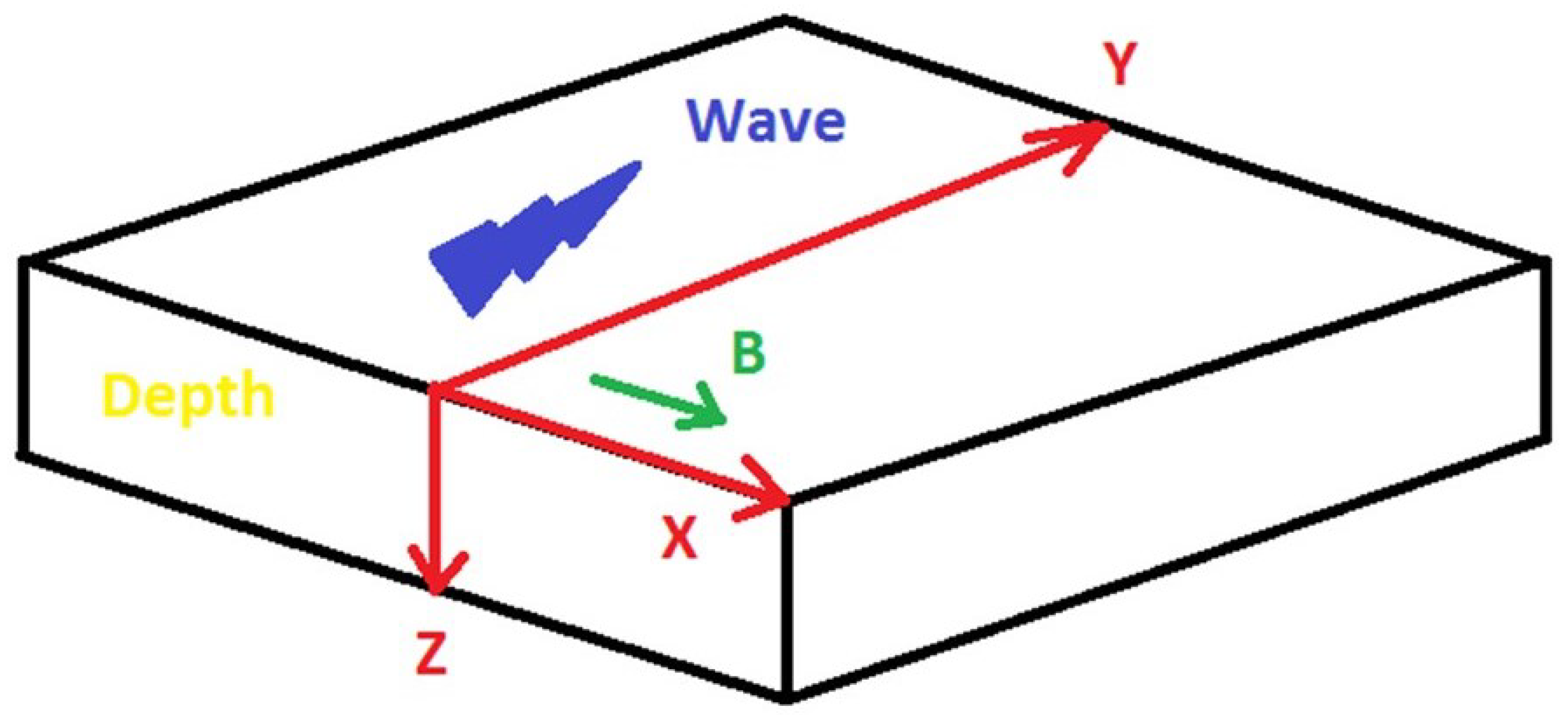
Replacing spherical geometry $(r,\theta ,\varphi )$ by a simple plain sheet $z,y,x$, we can obtain a simplified and visual model of the dynamo in the box, which is schematically shown in Figure 1. Here the magnetic field is directed along the x-axis, the dynamo wave propagates along the y-axis, and the depth of the convective zone is along the z-axis.

The equations in this case will take the form:

$${\displaystyle \frac{\partial A}{\partial t}}=\alpha B+\beta {\displaystyle \frac{{\partial }^{2}A}{\partial y^2}}+\beta {\displaystyle \frac{{\partial }^{2}A}{\partial z^2}}$$

(2)

$${\displaystyle \frac{\partial B}{\partial t}}=-{\displaystyle \frac{d{V}_x(y,z)}{dz}}{\displaystyle \frac{\partial A}{\partial y}}+\beta {\displaystyle \frac{{\partial }^{2}B}{\partial y^2}}+\beta {\displaystyle \frac{{\partial }^{2}B}{\partial z^2}}$$

(3)

B—toroidal magnetic field A—component of the vector potential describing the dipole magnetic field.

We represent time dependence for magnetic field as $e^{\gamma t}$, $\alpha$ and ${\displaystyle \frac{d{V}_x(y,z)}{dz}}$ are functions of z and y. The own solution of the equations is dynamo waves.

Since from the geometry of the problem we have only components $A_x$ and $B_x$, the equations take the form:

$${\displaystyle \frac{\partial A}{\partial t}}=\alpha B+\beta {\displaystyle \frac{{\partial }^{2}A}{\partial y^2}}$$

(4)

$${\displaystyle \frac{\partial B}{\partial t}}=-{\displaystyle \frac{d{V}_x(y,z)}{dz}}{\displaystyle \frac{\partial A}{\partial y}}+\beta {\displaystyle \frac{{\partial }^{2}B}{\partial y^2}}$$

(5)

In the linear case, when the $\alpha$-effect and differential rotation $\Omega$ are independent of the magnetic field amplitudes A and B, the behavior of the system is governed by a dimensionless parameter D, known as the dynamo number:

$$D={\displaystyle \frac{\alpha \Omega }{{\beta }^2{k}_y^3}},$$

where $k_y$ is the wave vector along the y-axis. At D less than $D_{cr}$ (threshold of dynamo generation) magnetic fields are dumped at opposite case dynamo process generates fields (exponential growth). For solar conditions $D_{cr}$ (threshold) is about several thousand uncertainty of knowing these parameters makes it difficult to conclude how far into super critical regime the actual solar dynamo is. That means we do not know how big is actual nonlinearity of dynamo is.

Nonlinear effects in dynamo are based on the following considerations: an increasing magnetic field begins to influence the character of the flow and thereby the condition for the dynamo of the process changes. It is believed that the most sensitive to nonlinearity is $\alpha$. The main non-linear effects are $\alpha$-coefficient modifications. There are still discussions on what its form should be [12].

In typical astrophysical cases such as the Sun and other stars, the dynamo number significantly exceeds the critical threshold for instability. As a result, higher-order modes with sufficiently large wave vectors k become unstable and can grow [13,14,15]. During the saturation phase, the magnetic field amplitudes are found to closely match the level required to fully compensate for the dynamo number’s excess above the instability threshold. This compensation arises through a nonlinear suppression of the $\alpha$-effect [16].

Let us introduce the concept of effective dynamo number, which describes the magnitude of the amplitude of the magnetic field generator at the current moment in time: $D_{eff}\left(t\right)=\alpha \left(t\right)\Delta V/\left({\beta }^2{k}^2\right)$, where nonlinear $\alpha$ is alpha-effect at the current moment in time, $\Delta V$ is the differential rotation jump at the thickness of the effective magnetic field generation layer. We will use this value in the next section.

3. Model of Solar (Stellar) Flare with Nonlinear Turbulent Diffusion

In the variety of magnetic activity of parent stars, a sufficiently large number have been discovered in which the flare energy significantly exceeds that we have on our Sun. Flares with energies up to ${10}^{36}$ erg were observed, which leaves far behind the most powerful event—the Carrington event with its ${10}^{32}$ erg. Accordingly, the amplitude of the magnetic field already recorded on some stars reaches up to several thousand Gauss, which, together with superflares, requires the dynamo mechanism to reach extreme amplitudes compared to the solar case [7,8,9]. The question arises as to what factors can determine the saturation values that the magnetic field reaches. There is no reason yet to believe that in other stars other physical processes other than solar ones are involved in the generation of the magnetic field, and it is quite natural to use already proven models of nonlinear saturation of magnetic field growth in the dynamo process.

For modelling we use the 1D Parker $\alpha \Omega$ dynamo model. We will assume that the nonlinear approximation of the alpha-effect should follow the already known algebraic suppression [12]. Turbulent diffusion can be nonlinear and depend on the magnitude of the magnetic field. To this, we will add nonlinear suppression of turbulent diffusion depending on the amplitude of the mean magnetic field:

$${\displaystyle \frac{\partial A}{\partial t}}=\alpha B+\beta {\displaystyle \frac{{\partial }^{2}A}{\partial {\theta }^2}}+{\displaystyle \frac{\partial \beta }{\partial \theta }}{\displaystyle \frac{\partial A}{\partial \theta }},$$

(6)

$${\displaystyle \frac{\partial B}{\partial t}}=-Dcos\theta {\displaystyle \frac{\partial A}{\partial \theta }}+\beta {\displaystyle \frac{{\partial }^{2}B}{\partial {\theta }^2}}+{\displaystyle \frac{\partial \beta }{\partial \theta }}{\displaystyle \frac{\partial B}{\partial \theta }},$$

(7)

$$\alpha ={\displaystyle \frac{{\alpha }_0}{1+B_{\alpha }^2{B}^2}},$$

$$\beta ={\displaystyle \frac{{\beta }_0}{1+B_{\beta }^2{B}^2}}.$$

Turbulent magnetic diffusion controls the diffusion of the magnetic field in the convective zone. We introduce a nonlinear suppression of this turbulent diffusion to account for the physical effect by which strong magnetic fields can suppress turbulent motions, thereby reducing the effective diffusion.

The dynamo model describes the generation and evolution of magnetic fields through the interaction between the $\alpha$-effect and differential rotation, while turbulent diffusion controls how these fields are spatially redistributed and dissipated over time. The evolution of the magnetic field is governed by the balance between amplification (via dynamo action) and diffusion (via turbulent processes). Therefore, including a nonlinear dependence of diffusion on field strength allows us to capture saturation effects and local energy accumulation, which are crucial for modeling flares and superflares. Algebraic suppression of helicity and turbulent diffusion is considered as the simplest and quite working scheme of suppression of alpha-effect and turbulent diffusion with increasing amplitude of magnetic field. Since the our dynamo model itself is one-dimensional and qualitative, for the primary analysis it is possible to suggest that such assumptions are sufficient. In more complex dynamo models it is possible to introduce dynamic suppression of helicity and turbulent diffusion, where they would be unknown functions of dynamo equations and their evolution could be found from the general picture of magnetic field generation. Since our model is qualitative, the most important for us is the relative change of magnetic field in the model: for example, switching of the mode from a regular cycle to a cycle, where there are regions of extreme growth of magnetic field in comparison with its maxima in a regular cycle.

It is convenient to characterize, the intensity of the $\alpha$-effect and differential rotation, as triggers of the dynamo process in terms of dimensionless parameters $R_{\alpha }=\left({\alpha }_{*}R\right)/\beta$ and $R_{\Omega }=\left(G_{*}{R}^3\right)/\beta$. Here R—characteristic space scale of the dynamo region in the star (the thickness of the convective layer in the case of the Sun), ${\alpha }_{*}$ and $G_{*}$—average values of $\alpha$ and G in dynamo zone (to reflect the intensity of generation of poloidal and toroidal fields respectively. $D=R_{\alpha }{R}_{\Omega }$ in this case. In system (1) and (2), time and distances are measured in dimensionless units, which are introduced when constructing the dynamo number.

In Equations (6) and (7), both time and spatial variables are expressed in dimensionless units, as defined during the formulation of the dynamo number. Specifically, the time unit is not in conventional years but is based on the so-called diffusion time—the characteristic timescale over which a fluid element traverses the convective zone due to turbulent diffusion. This diffusion time is estimated as ${\displaystyle \frac{d^2}{\beta }}$, where d represents the thickness of the convective layer and $\beta$ is the turbulent magnetic diffusivity. The magnetic field itself is also normalized, typically measured in units corresponding to the amplitude at which nonlinear saturation of the dynamo occurs. This saturation level is generally associated with an approximate equipartition between the turbulent kinetic energy and magnetic energy [16].

Here we use the simplest scheme for stabilizing the growth of the magnetic field, the so-called suppression of helicity. Within the framework of this scheme, it is assumed that $\alpha ={\alpha }_0\left(\theta \right)/(1+{B_{\alpha }}^2{\mathbf{B}}_0^2)$, where ${\alpha }_0$ is the helicity value in a non-magnetized medium, and ${\mathbf{B}}_0={B_{\alpha }}^{-1}$ is the magnetic field at which the alpha-effect is significantly suppressed. For definiteness, we assume that ${\alpha }_0=sin\left(\theta \right)$. In the expression for the suppression of turbulent diffusion, we have magnetic field ${\mathbf{B}}_0={B_{\beta }}^{-1}$ at which the turbulent diffusion is significantly suppressed and the turbulent diffusion ${\beta }_0$ in a non-magnetized medium.

As boundary conditions we use the conditions $A(-\pi /2)=B(-\pi /2)=A(\pi /2)=B(\pi /2)=0$, which corresponds to dipole symmetry. The factor $cos\left(\theta \right)$ in the second equation corresponds to the decrease in the length of the parallel near the pole. We use a small seed field as initial conditions.

We will study the problem for the case where the presence of algebraic suppression of turbulent diffusion will change the picture of the regular solar (stellar) cycle. In our problem, to simulate this, we consider the constant parameter $D=-400$.

We solved the system numerically using a set of codes on Wolfram Mathematica.

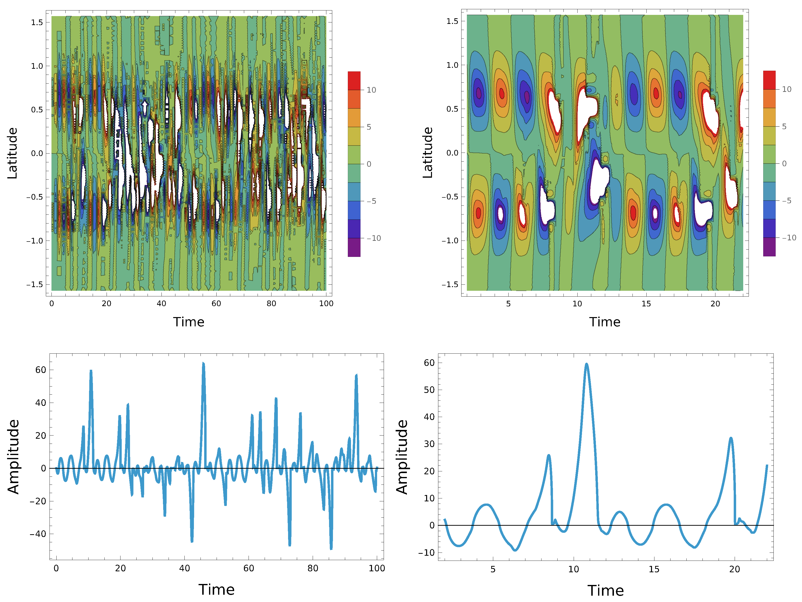
The Figure 2 shows the latitude-time dependences for the toroidal magnetic field in the case of constant turbulent diffusion - the upper panel. On the left is the magnetic field for a long period of time, during which many reversals of the magnetic field occur. On the right is a shorter time interval to show the magnetic field in cycles in more detail. Here the stellar cycle is regular. The lower panel corresponds to the dependence of the amplitude of this toroidal magnetic field on time at the latitude $\pi /6$. The amplitude of turbulent diffusion is $0.63$. Here and further time is given in dimensionless diffusion units, which are described above. Here, the period of magnetic activity corresponds in order to the solar one. Latitude is given in radians. Magnetic field amplitude is given in units corresponding to the amplitude at which nonlinear saturation of the dynamo occurs. In our case, for the regular cycle in Figure 2, at its maximum this corresponds approximately to the amplitude of the magnetic field in a sunspot of the order of several thousand Gauss.

The Figure 3 shows the latitude-time dependences for the toroidal magnetic field in the case of nonlinear turbulent diffusion—the upper panel. Similar to Figure 2, on the left is the magnetic field for a long period of time, during which many reversals of the magnetic field occur. On the right is a shorter time interval to show the magnetic field in cycles in more detail. The lower panel corresponds to the dependence of the amplitude of the toroidal magnetic field on time at a latitude of $\pi /6$. The coefficient ${\beta }_0=1$, $B_{\beta }^2=0.065$. In this case, regions with a magnetic field amplitude significantly exceeding the magnetic field in a regular cycle randomly appear - white zones. The lower panel shows the time moments with such peaks. Such regions in our model correspond to flare regions. 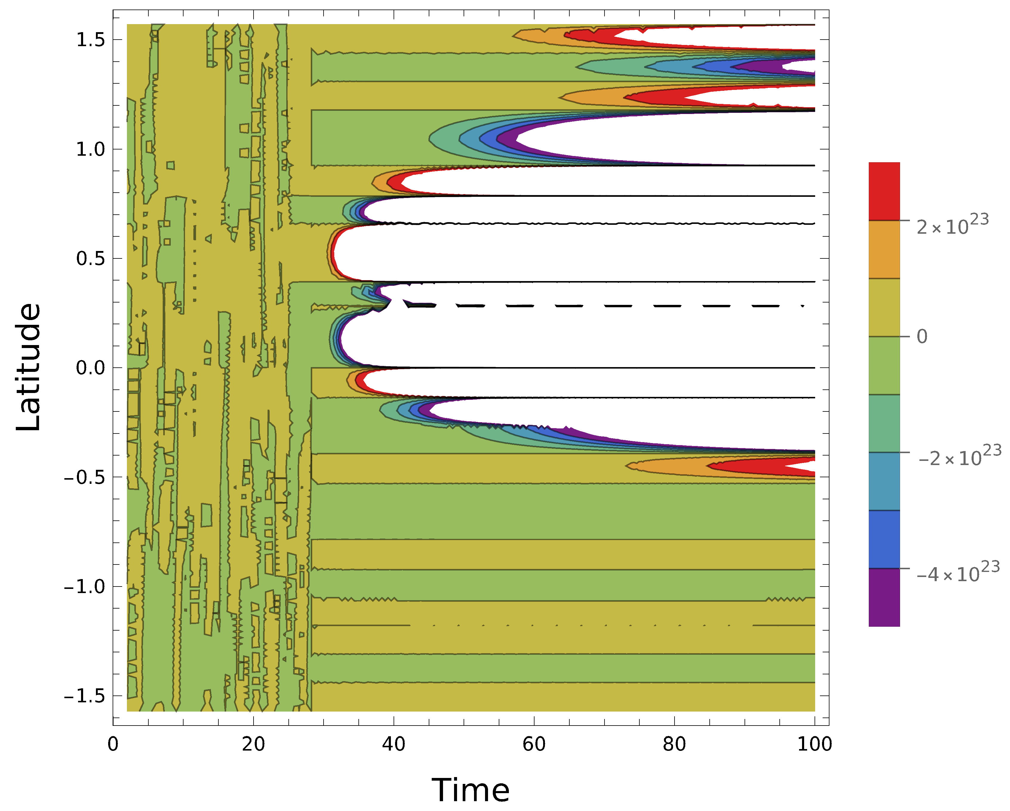With a decrease in $B_{\beta }^2$, the flares disappear (in this case latitude-time dependence for the toroidal magnetic field looks like upper panel in Figure 2), and with an increase to about 0.1, the regions gradually grow and with a further increase in nonlinearity, large regions of a large magnetic field appear that no longer disappear as shown in the Figure 4 for $B_{\beta }^2=0.2$. If at $B_{\beta }^2=0.065$ a flare occurs once every few stellar cycles, then as it increases, flares occur almost every cycle.

We assume that in reality there may be a rather weak nonlinearity in turbulent diffusion, which varies depending on the age of the star. The bottom panel clearly shows how the amplitude of the magnetic field increases during the flare and, accordingly, its energy.

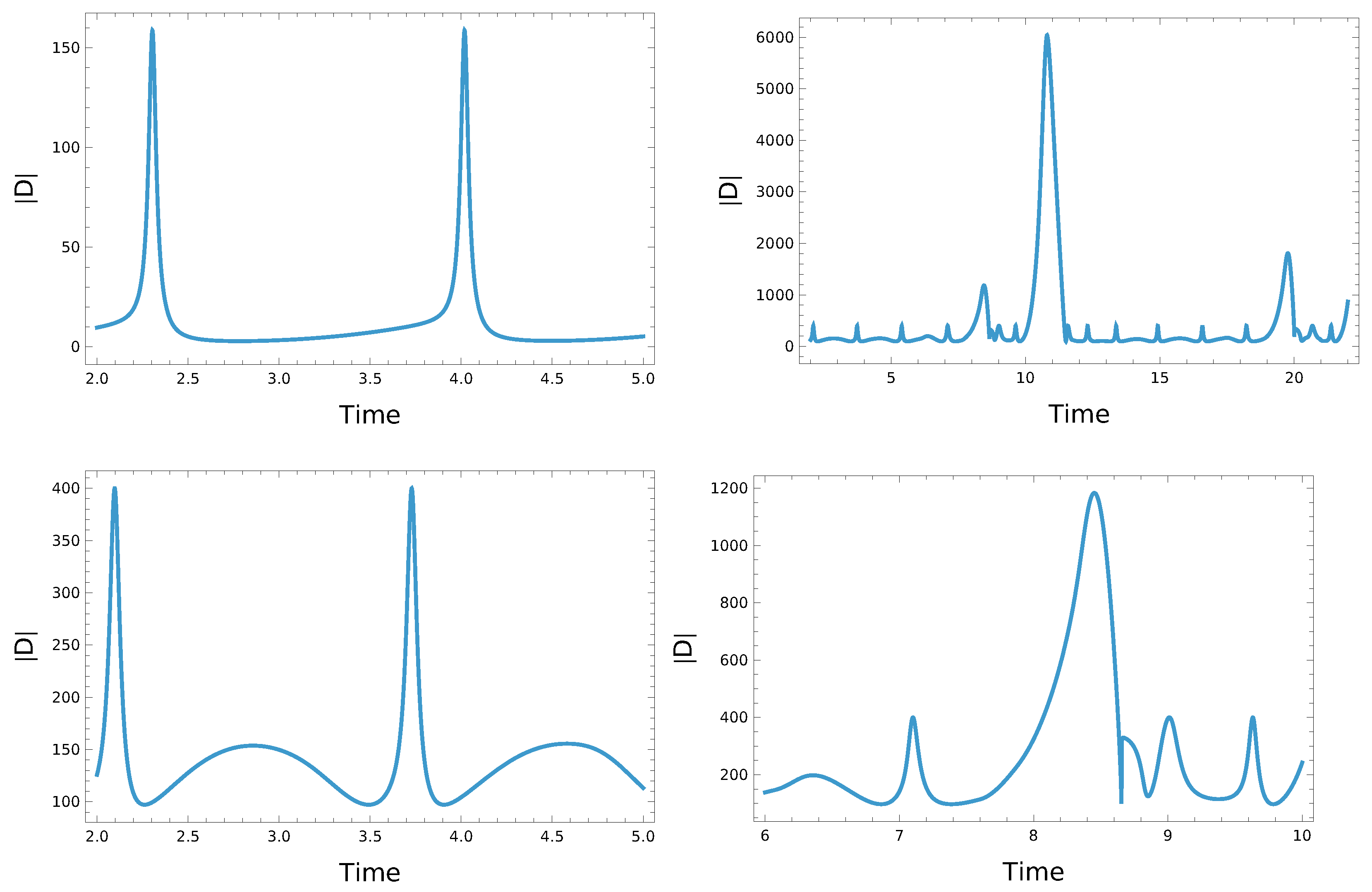
In the Figure 5, the left upper panel shows the dependence of the effective dynamo number module on time in the case of constant turbulent diffusion, corresponding to the above. The right upper panel shows a similar dependence for the case of nonlinear turbulent diffusion. The left lower panel represents the time interval with regular activity for nonlinear case, the right lower panel corresponds to the moment of the flare. The effective dynamo number corresponds to the magnetic field growth factor at a given time. The upper left panel displays the regular increase and decrease of the magnetic field, characteristic of cyclic activity. The upper right panel displays the change in the magnetic field growth during flare activity, which occurs due to the inclusion of nonlinearity in turbulent diffusion. Note that the lower left and right panels are enlarged sections of the upper right panel. The lower left panel shows that even during a regular cycle, small fluctuations in the latitudinal dependence of the magnetic field maxima distribution occur. This is also evident if we compare the upper right panels of Figure 2 and Figure 3. In Figure 3, it is clear that the “Maunder butterflies” shift slightly from cycle to cycle along the latitude. This corresponds to real solar and stellar cycles. The lower right panel in Figure 5 shows how the field grows during the flare.

We assume that the numerical value of the dynamo generation threshold for real differential rotation profiles and others may significantly differ from the simplified model. This is confirmed by comparing the results of a dynamo in a box with more complex 3D MHD simulations for realistic choices of spatial profiles of the spatial distribution of the alpha-effect, differential rotation, and turbulent magnetic diffusion [12]. Even in the case of the solar dynamo to find the full set of all those profiles is still a problem (despite continuous efforts in helioseismology). There is no way to launch such a comprehensive approach as in the case of other stars, when in the vast majority of stars from the KEPLER and TESS catalogs, we are left only with basic data on luminosity history. However, simplified models are very useful in that they help to obtain a qualitative picture of the influence of a particular factor on the process of magnetic field generation and to identify what physical effects may arise. Such results of numerical and analytical studies of simplified models can be used in more detailed 3D modeling.

4. Discussion

There are different types of dynamo models that can describe the irregularity of the solar cycle, which can be indirectly related to flare activity. Stochastic dynamo models include random or periodic excitation of the $\alpha$-effect, stochastic modulation of the dynamo parameters (e.g., $\alpha \left(t\right),\Omega \left(t\right)$). Flares can arise due to sharp changes in the parameter values, which lead to instabilities, resonant pumping or transitions between field modes [17]. Dynamo models with nonlinear feedback and delay, where, for example, a time delay in $\alpha$ or other parameters is introduced and this causes accumulation of instability, then a sharp release of energy. Quasiperiodic flares with a characteristic cycle of accumulation and breakdown occur [18]. Magnetohydrodynamic (MHD) 3D dynamo simulations, where irregularity of the solar cycle occur spontaneously if realistic diffusion, magnetic reconnection, and feedback are included [19,20]. The model we propose, on the one hand, uses a physical mechanism where natural suppression of turbulent diffusion occurs due to an increase in the amplitude of the magnetic field, which is used in local MHD modeling. The novelty of our model is that we tried to combine the consideration of local effects in a large-scale dynamo. Our model can be attributed to the types of models that help in the further development of 3D models with an emphasis on studying the details of the turbulent diffusion process.

We built a model for the occurrence of flares and superflares, which can be verified with the help of observations of stellar activity. As can be seen from the Figure 3, the amplitude of the flares can be different, which can correspond to both small flares and super flares. The magnetic field energy, proportional to $B^2$, in these flares can exceed the maximum energy in a regular cycle by tens of times. Since the model is qualitative and rather simplified, the flare areas are quite large compared to the duration of the cycle. However, such a model allows us to see the main trends in the behavior of the magnetic field.

We investigated the problem on different ranges of dynamo numbers. For the pattern of flares to occur, the dynamo number must exceed the generation threshold so that the field can be generated, but it must not exceed it too much. In fact, in our model, the dynamo number is several hundred. As the dynamo number in our model increases, the flares become so strong (the effective dynamo number (which corresponds to the growth factor of the magnetic field at a given moment in time) during them increases by orders of magnitude) that the star cannot return to the normal cyclic activity mode.

We assume that superflares are a result of a faster axial velocity of stellar rotation, which makes stronger alpha-effect and differential rotation, together generating growing dynamo fields in convection zones. Star spots are the result of magnetic flux tubes rising under magnetic field pressure, transferring a stronger field to the photosphere and chromosphere. Overall, a more detailed analysis of the existing KEPLER, TESS, and EVRY data provides a resource for developing models of flares occurring on different types of stars, both fully convective and with different thicknesses of the convective zone. The size of the star spot and the amplitude of the “surface” magnetic field determine the upper limit of the energy output for superflares. A very powerful superflare, as we suggest on the basis of our modeling, is capable of generating magnetic fields so high that they can suppress the amplitude of turbulence in the convective zone, thereby blocking the heat transfer regime vital for the thermal balance of the star. This thermal convective blocking creates a local “superheated boiler explosion” mechanism. To describe the balance of suppression of the star’s flare activity, we found that it is possible to introduce a nonlinear damping for the turbulent magnetic diffusion coefficient. Note that in our model, flare regions with a larger area generally have a stronger magnetic field than the field in small flare regions.

Flares occur in active regions with a local magnetic field of about 100–1000 gauss, superflares are associated with a more powerful magnetic field, which can reach 5000 gauss and more. Our results, see Figure 3 bottom panel, qualitatively reproduce this relationship between the fields in a regular cycle and during flares of different magnitudes. In the observational data, flares are visible on the light curves: a normal flare, see Figure 4 in [21], light curves of the example superflares on Sun-like stars can be seen in Figure 2 in [22].

RS CVn-type stars represent particularly valuable targets for verifying our model, due to their well-documented photometric variability and high flare activity. They are known for their high levels of magnetic activity, including frequent and energetic flares. In recent years (see, for example, [23]), data on the motion of plasma in these stars has appeared, which provides the prospect of verifying our model on these objects. The observed cyclic behavior and flare activity in RS CVn stars suggest that variations in surface differential rotation and nonuniform turbulent diffusion contribute to localized magnetic field amplification.