Article

Core–Corona Decomposition of Very Compact (Neutron) Stars: Accounting for Current Data of XTE J1814-338

by
Rico Zöllner
1,*,† and
Burkhard Kämpfer
2,3,†
1
Institut für Technische Logistik und Arbeitssysteme, TU Dresden, 01062 Dresden, Germany
2
Helmholtz-Zentrum Dresden-Rossendorf, 01314 Dresden, Germany
3
Institut für Theoretische Physik, TU Dresden, 01062 Dresden, Germany
*
Author to whom correspondence should be addressed.
These authors contributed equally to this work.
Astronomy 2025, 4(2), 10; https://doi.org/10.3390/astronomy4020010
Submission received: 14 March 2025 / Revised: 17 April 2025 / Accepted: 20 May 2025 / Published: 9 June 2025

Abstract

:
A core–corona decomposition of compact (neutron) star models was compared with the current mass–radius data of the outlier XTE J1814-338. The corona (which may also be dubbed the envelope, halo or outer crust) is assumed to be of Standard Model matter, with an equation of state that is supposed to be faithfully known and accommodates nearly all other neutron star data. The core, solely parameterized by its mass, radius and transition pressure, presents a challenge regarding its composition. We derived a range of core parameters needed to describe the current data of XTE J1814-338.

1. Introduction

The pulse-profile modeling of the accretion-powered millisecond pulsar XTE J1814-338 by a single uniform-temperature hot-spot resulted in mass (M) and radius (R) parameters of ( R / km , M / M ) = ( 7.0 0.4 + 0.4 , 1.21 0.05 + 0.05 ) [1]. In particular, the extraordinarily small radius poses a problem for establishing a proper neutron star model based on a unique equation of state (EoS) that is compatible with other compact (neutron) star data. The latter ones are provided by gravitational waves from merging neutron stars, the related multi-messenger astrophysics and the improving mass–radius determinations, in particular those by NICER data (see Appendix A in [2] for a survey and relationship to other data). Canonical neutron star radii are centered at about 12 km . Indeed, ref. [3] quotes R = 12.45 0.65 + 0.65 km for a 1.4 M neutron star and R = 12.35 0.75 + 0.75 km for a 2.08 M neutron star. HESS J1731-347 with ( 10.4 0.78 + 0.86 , 0.77 0.17 + 0.20 ) [4] may be another outlier with respect to mass1, as the black widow pulsar PSR J0952-0607 may also be, which points to a large mass of 2.35 0.17 + 0.17 M [6], with implications studied in [7].
The problem of XTE J1814-338 is addressed in [8,9,10,11,12,13]. Various proposals have been forwarded thereby, including various forms of Dark Matter (DM) admixtures and a strong first-order phase transition in Standard Model (SM) matter at supra-nuclear densities (see also [14] for an avenue toward ultra-compact hybrid stars). Scenarios with DM components offer a multitude of set-ups, e.g., including fermionic or bosonic or mirror matter in various constellations.
Instead of adding another specific model of the matter composition to explain XTE J1814-338 in terms of the mass and radius, here we followed an agnostic approach, outlined in [2,11,15], known as the core–corona decomposition (CCD). This approach can be imagined as a subdivision of a compact (neutron) star into two parts—the core, embedded in the corona2. The core is solely parameterized by its radius, mass and surface pressure. The latter one supports the corona, which, by definition, is composed of SM matter only, with a known equation of state (EoS). Imposing a hydrodynamic equilibrium of the isotropic corona fluid, the Einsteinian equations for spherical symmetry completely govern the corona structure. Either uncertainties of the supra-nuclear EoS or unknown DM admixtures (or other exotic non-SM matter effects) or both are not explicitly dealt with but are completely condensed into the three core parameters. The motivation of this approach is isolated and quantifies lesser or uncertainly known features of matter in the deep interior of a compact star with the hope of receiving hints about their nature. If a core is not required or one meets a “trivial core” (this notion is explained below), the conventional approach to spherically symmetric static and compact stars is recovered.
Our note is organized as follows. Section 2 outlines the CCD. A comparison of the CCD with data is presented in Section 3, where we include XTE J1814-338 as a compact object with a large massive core (which may contain a DM component or/and a special SM material component). We also put emphasis on the mapping of the credibility regions of masses and radii to the inferred core masses and radii. Section 4 provides a brief comment on two particular core models, one based on a statistically determined EoS from multi-messenger data and another one accommodating a strong first-order phase transition. We summarize in Section 5. Appendix A deals with an example where no core is required. For the sake of self-containment, a few results from [11] are recollected, where an extensive bibliography can be found.

2. Outline of Core–Corona Decomposition

The standard modeling approach of compact star configurations is based on the Tolman–Oppenheimer–Volkoff (TOV) equations
d p ( r ) d r = G N [ e ( r ) + p ( r ) ] [ m ( r ) + 4 π r 3 p ( r ) ] r 2 [ 1 2 G N m ( r ) r ] ,
d m ( r ) d r = 4 π r 2 e ( r ) ,
resulting from the energy–momentum tensor of a static isotropic fluid (described locally by pressure p and energy density e, which are solely relevant for the medium) and the spherical symmetry of both space-time and matter within the framework of Einsteinian gravity without the cosmological term [16]. Newton’s constant is denoted by G N , and natural units with c = 1 are used, unless when relating mass, length, pressure and energy density, where c is needed.
Given a unique relationship between the pressure p and the energy density e in the EoS e ( p ) , in particular at zero temperature, the TOV equations are customarily integrated (e.g., with the Runge–Kutta algorithm) with boundary conditions p ( r ) = p c O ( r 2 ) and m ( r ) = 0 + O ( r 3 ) at small radii r, and p ( R ) = 0 and m ( R ) = M , with R as the circumferential radius and M as the gravitational mass (acting as parameters in the external (vacuum) Schwarzschild solution at r > R ). The quantity p c is the central pressure. The solutions R ( p c ) and M ( p c ) provide the mass–radius relationship in the parametric form M ( R ) , being a curve.
Here, we employed another approach [2,11,15]. We parameterized the supra-nuclear core by a radius r x and the included mass m x and integrated the above TOV equations only within the corona, i.e., from pressure p x to the surface, where p = 0 . This yielded the total mass M ( r x , m x ; p x ) and the total radius R ( r x , m x ; p x ) by assuming that the corona EoS p ( e ) was reliably known for p p x and only SM matter occupied the region r r x . Clearly, without any knowledge of the matter composition at p > p x (may it be SM matter with an uncertainly known EoS or may it contain a DM admixture, for instance, or monopoles or some other type of “exotic” matter), one does not obtain a simple mass–radius relationship by such a procedure, but admissible area(s) over the mass–radius plane, depending on the core parameters r x and m x and the matching pressure p x and related energy density e x 3. This is the price of avoiding a specified model of the core matter composition. However, the CCD is a simple and efficient approach to quantify the appearance of some “exotics” by a displacement from the mass–radius curve related to an SM matter EoS. For an SM matter-only core with EoS p SM ( e ) , the core parameters are strongly correlated, m x ( p c ) , r x ( p c ) for p c p x , thus yielding masses and radii near to or on the M ( R ) curve provided by p SM ( e ) . The limits r x 0 , m x 0 and p x p c reduce the CCD in the conventional one-fluid TOV equations.
Note that our core–corona approach relies on the assumption that the region r [ r x , R ] is occupied only by SM matter with a trustable EoS. Thus, scenarios as in [8], where bosonic DM forms a halo around a core with SM + DM components, are not captured by our CCD.

3. Catching Current Data of XTE J1814-338 by CCD

3.1. Selecting a Reference EoS

The NICER data of PSR J0437-4715 [18], ( R / km , M / M ) = ( 11.36 0.63 + 0.95 , 1.42 0.04 + 0.04 ) and PSR J0740+6620 [19], ( 12.49 0.88 + 1.28 , 2.073 0.069 + 0.069 ), exhibited in Figure 1 in [11], clearly demonstrate that the EoS NY Δ 4 in [17] satisfactorily matches these data. However, it falls short in the maximum mass of the black widow pulsar PSR J0952-0607, which points to a large mass of 2.35 0.17 + 0.17 M [6] with implications studies in [7]. More (NICER) data are mentioned in Appendix A in [11] to exhibit the usefulness of NY Δ , which, however, fails badly for the outlier XTE J1814-338 [1] and still shows some tension with ( 10.4 0.78 + 0.86 , 0.77 0.17 + 0.20 ) for HESS J1731-347 [4], which may be another outlier or a hint of twin stars [20]. We focus here on a description of XTE J1814-338, ( R / km , M / M ) = ( 7.0 0.4 + 0.4 , 1.21 0.05 + 0.05 ) [1], by CCD. Rotational effects are assumed to be subleading.

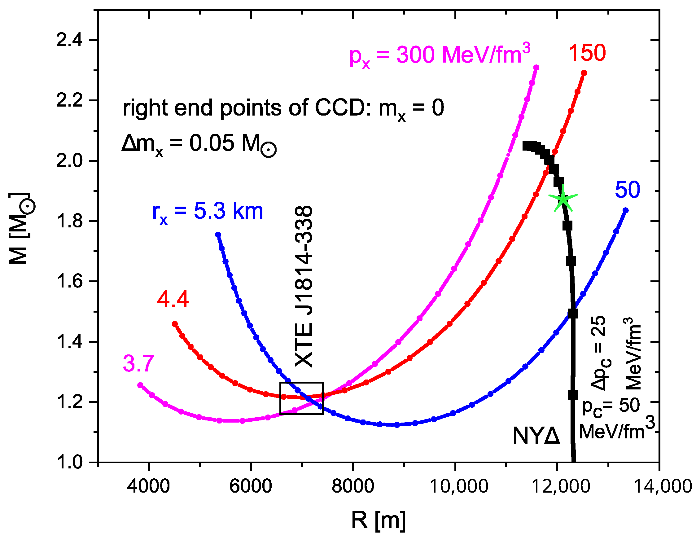
3.2. Masses and Radii

The credibility region of XTE J1814-338 was according to [1] mass M M XTE ± Δ XTE ( M ) s ¯ and radius R R XTE ± Δ XTE ( R ) s ¯ with M XTE = 1.21 M , Δ XTE ( M ) = 0.05 M , R XTE = 7.0 km , Δ XTE ( R ) = 0.4 km and s ¯ = 1 . We named this region “XTE square”. Occasionally, we also considered the “XTE ellipsis”:
s Δ XTE ( M ) 2 ( M M XTE ) 2 + s Δ XTE ( R ) 2 ( R R XTE ) 2 = 1 .
In both cases, the parameters s ¯ and s are meant to steer an assumed accuracy or to describe the credibility level.
Selecting core–surface pressures p x = 50 , 150 and 300 MeV / fm 3 and core radii r x = 5.3 (blue curve), 4.4 (red curve) and 3.7 km (magenta curve), one finds good descriptions of the XTE square for suitable values of core masses; see Figure 1. The curves were generated by running values of m x from zero (right end points) to larger values by steps of Δ m x = 0.05 M in going left. In addition, the mass–radius relationship for NY Δ without any core is exhibited by the solid black curve. Filled squares are for p c = 25 n MeV / fm 3 for n = 2 , , 14 . The asterisk exposes the point with p c = 150 MeV / fm 3 .
By replacing the XTE square with s ¯ = 1 with XTE ellipses, one finds the regions of core masses m x and core radii r x displayed in Figure 2 for a sequence of selected values of p x = 50 , 100 , 150 , 250 and 350 MeV / fm 3 . The parameters were set to s = 1 (solid curves), 2 (dotted curves) and 4 (double lines). The centers of the displayed ellipses approximately obeyed m x ( 0.33 + 0.14 r x km ) M , which allowed space for m x 0.33 M when extrapolated to r x 0 . That is, the core compactness C x = 2 G N m x / r x 0.42 + km r x increased with increasing core–boundary pressure p x . For instance, C x | 350 MeV / fm 3 0.7 was much larger than the total XTE compactness of 0.52. The core masses scaled with p x as m x 1.513 log ( p x / [ MeV / fm 3 ] ) M .
Replacing the credibility ellipses with squares, the ellipses turned into parallelograms with envelopes approximately obeying m x ( a + b r x ) M with a = 0.262 , b = 0.1366 / km (lower tips) and a = 0.3266 , b = 0.1566 / km (upper tips), which leaves space for m x [ 0.262 , 0.3266 ] M when extrapolated to r x 0 .

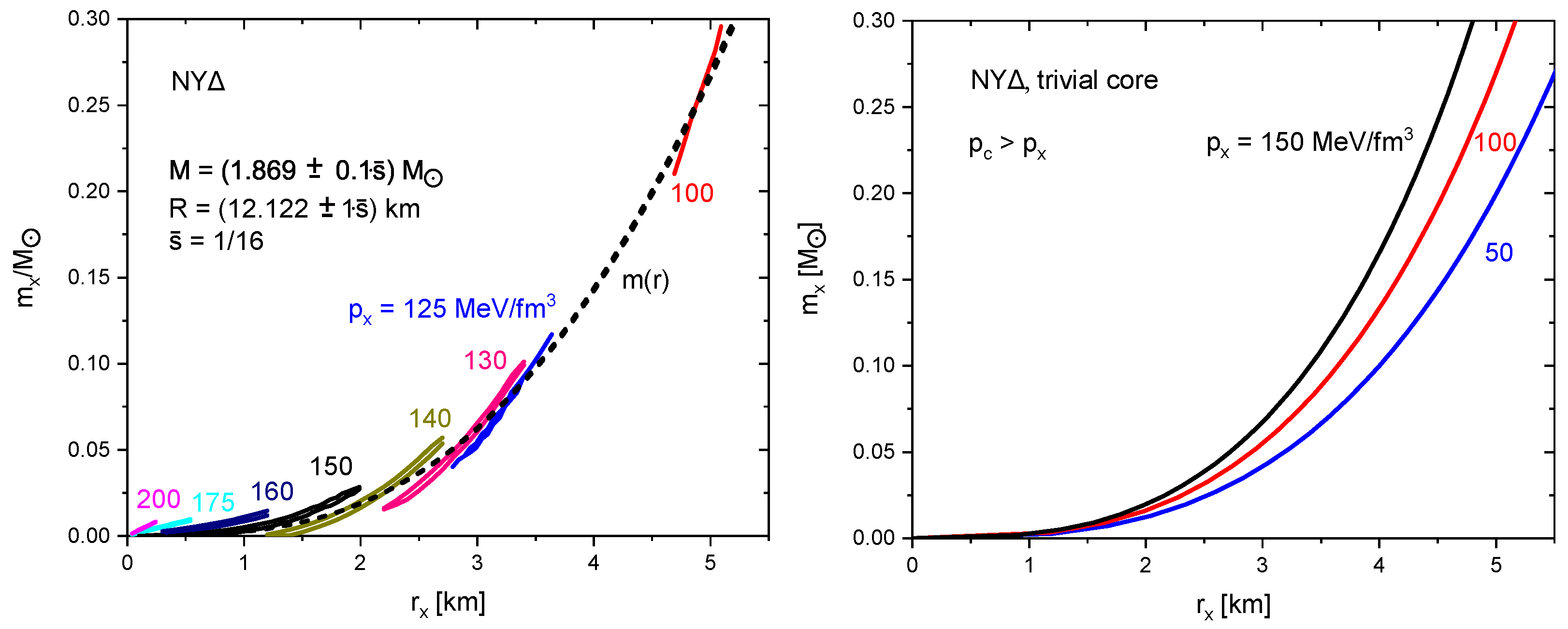
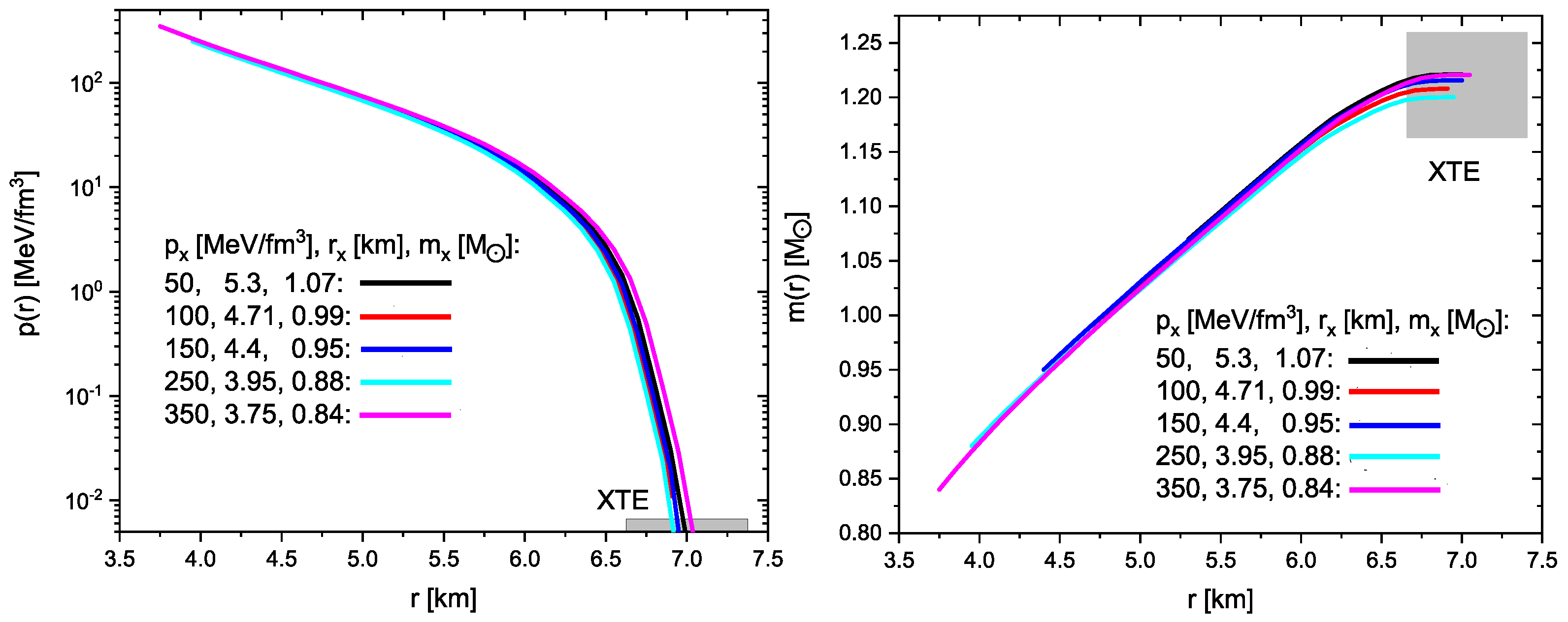
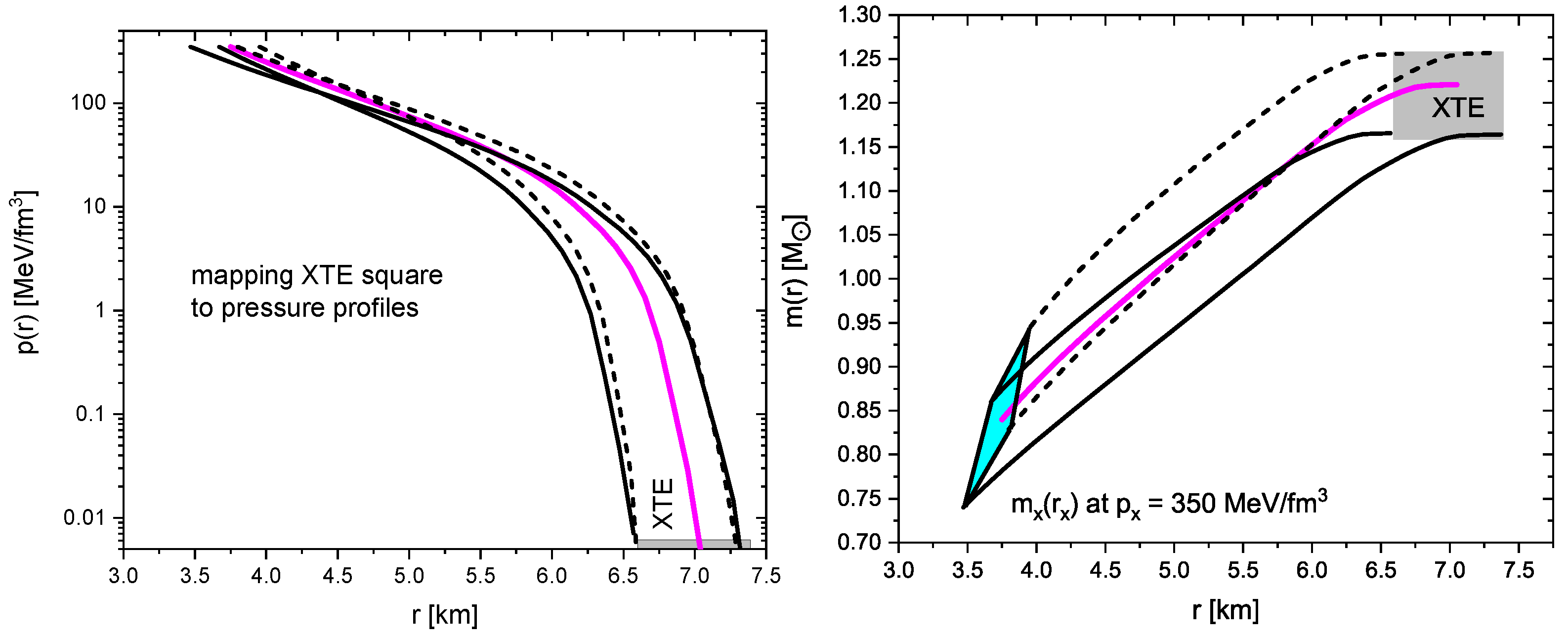
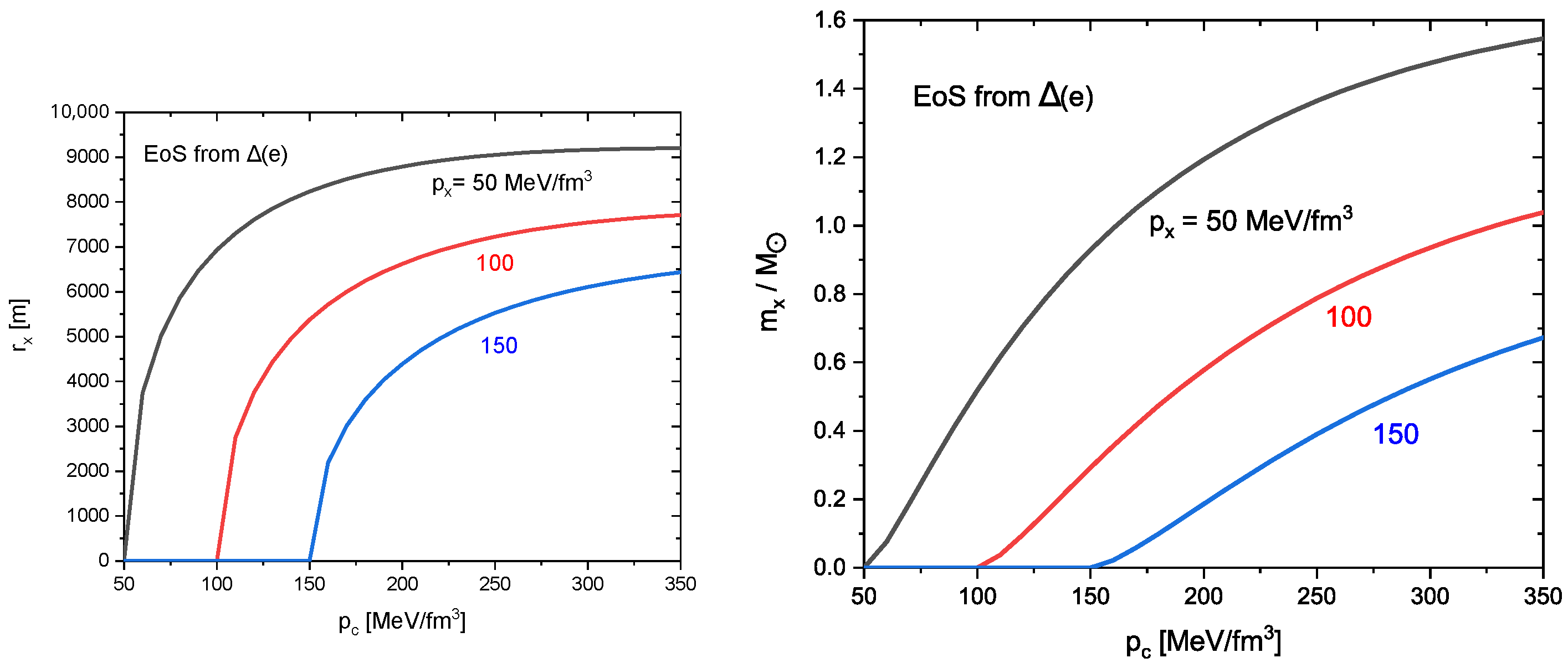
3.3. Pressure and Mass Profiles in the Corona

The pressure and mass profiles are exhibited in Figure 2 in [11], also including the case of the HESS remnant J1731-347, both for p x = 50 MeV / fm 3 . Here, we display in Figure 3 the profiles for p x = 50 , 100 , 150 , 250 and 350 MeV / fm 3 for XTE J1814-338 only. In doing so, by the shooting method, we select the core parameters ( p x / ( MeV / fm 3 ) , r x / km , m x / M ) = ( 50 , 5.3 , 1.07 ) (black curves), ( 100 , 4.71 , 0.99 ) (red curve), ( 150 , 4.4 , 0.95 ) (blue curve), ( 250 , 3.95 , 0.88 ) (cyan curves) and ( 350 , 3.75 , 0.84 ) (magenta curves), which deliver ( M , R ) within the XTE square. Both the pressure profiles and the mass profiles are nearly on top of each other, suggesting the occurrence of a master curve, which could be obtained by inward integration. However, NY Δ is limited to p 373.58 MeV / fm 3 , i.e., larger values of p x are not accessible.
Analog master curves map the corners of the XTE square to p ( r ) and m ( r ) ; see Figure 4. This accomplishes the mapping of the XTE square ↦ ( m x , r x ) | p x . One admissible parallelogram is shown for p x = 350 MeV / fm 3 in the right panel. For each value of p x , a corresponding parallelogram can be constructed by combining the information depicted in both panels. Figure 2 above uses XTE ellipses and a few discrete values of p x . The mentioned approximations refer to the upper dashed and lower solid curves in Figure 4(right).

4. Considering One-Fluid Core Examples

The CCD was useful for isolating the details of the corona. What remained for further progress was to attempt an explanation of the core parameters ( p x , r x , m x ) . As pointed out in the previous subsection, one has to employ another EoS in the region of p > 350 MeV / fm 3 . We now test two examples for a core EoS: (i) an EoS related to the QCD trace anomaly (Section 4.1) and (ii) a strong first-order phase transition (Section 4.2). Both examples assume the applicability of the above one-fluid TOV equations.

4.1. Using Core Model with EoS Related to QCD Trace Anomaly

To present an explicit example of a one-fluid core, we adapt the EoS related to the QCD trace anomaly Δ , i.e., p ( e ) = e [ 1 3 Δ ( e ) ] and squared sound velocity v s 2 = 1 3 Δ e Δ e . In [21], Δ ( e ) is statistically determined with constraints from multi-messenger neutron star data with respect to hints of approaching conformality in the cores. Δ ( η ) with η : = ln ( e / 150 MeV / fm 3 ) , originally proposed in [22], agreed—with a tiny correction of one parameter—with Δ NY Δ ( η > 0.9 ) from [17]; see Figure 3—left in [2]. The plots of Δ ( e ) and v s 2 ( e ) in [21] (see Figure 4 there) can be parameterized by
Δ = 0.33 1 A 1 + exp { κ ( η η c ) } + G G exp ( η η G ) 2 2 σ G
with η : = ln ( e / e ^ 0 ) , e ^ 0 = 0.12 GeV / fm 3 , A = 1.52 , κ = 3.582856 , η c = 1.357143 , G G = 0.2926 , η G = 4.045714 and σ G = 2 .
The one-fluid TOV equations are integrated from r = 0 , where p = p c and m = 0 , to r x , where p ( r x ) = p x and m x = m ( r x ) . The emphasis here is placed on the non-trivial dependence of both Δ ( e ) and v s 2 ( e ) , which encode the EoS. The corresponding core radii and masses as functions of the central pressure p c are shown in Figure 5. Both core radii and core masses increased with central pressure. (For comparison, somewhat smaller values of r x ( p c ) and m x ( p c ) would have been obtained when using NY Δ as a core EoS.) Note that, for a one-fluid core with a given EoS and p x , the values of r x and m x become correlated due to the p c dependence, and the usual stability criteria apply5.
This example of a one-fluid core model did not deliver consistent values of r x ( p c ; p x ) and m x ( p c ; p x ) at p x = 50 , 100 and 150 MeV / fm 3 , which were needed—in combination with the NY Δ corona model—to match the XTE J1814-338 data [1]; see Figure 6. For XTE J1814-338, a more compact core is required, which could be accomplished using a DM admixture by a strong first-order phase transition (FOPT).

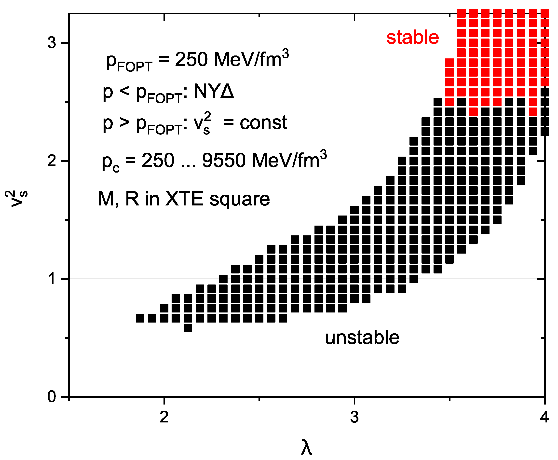
4.2. First-Order Phase Transition

In this subsection, we consider an example of an FOPT. That is, the NY Δ EoS is continued at p > p FOPT by a constant sound velocity model EoS. Following [10], we continue the NY Δ EoS at p > p FOPT = 250 MeV / fm 3 with
e ( p ) = λ e NY Δ ( p FOPT ) + v s 2 ( p p FOPT ) .
This choice of p FOPT left the stable NY Δ branch unaffected (see the bold solid black curve in Figure 1) with R 12 km and masses up to 2.02 M , thus being (marginally) consistent with many gravitational waves, multi-messengers and NICER observations. A sufficiently strong FOPT with an energy density jump parameterized by λ at p FOPT and constant sound velocity squared v s 2 at p > p FOPT initially bent the M ( R ) curve down. For running p c up to extraordinarily large values in the order of 10 GeV / fm 3 , one could catch the XTE square (see Figure 1). Figure 6 shows the region v s 2 vs. λ , where M and R fall in the XTE square. In contrast to [10], our EoS combination did not allow for stable compact (neutron) stars with causal high-density EoS.
Despite this failure, attention may still be directed toward core-only properties and use the above EoS construction. Keeping p FOPT = 250 MeV / fm 3 and selecting p c = 5 GeV / fm 3 together with λ = 2.9 and v s 2 = 1 , we determined the corresponding core, i.e., radii r x determined by p ( r x ) = p x . Interestingly, for p x = 50 , 100 , 150 and 250 MeV / fm 3 , the core–mass–core–radius relationship was approximately m x ( 0.33 + 0.14 r x km ) M , which matched the p x dependence of the XTE ellipse centers displayed in Figure 2. That is, such a model EoS and such a p c choice would have served as a specific core model. The special case of p x = 250 MeV / fm 3 is a model with a core as a high-density EoS and a corona as nuclear (NY Δ ) matter, both joined by an FOPT.
Both examples demonstrate that a one-fluid SM matter core is unlikely to explain the required core parameters for XTE J1814-338. In Appendix A, we consider the special case of a “trivial core”, which means that a distinguished core is not needed.

5. Summary

The CCD relied on the agnostic assumption that the EoS of compact (neutron) star matter (i) was reliably known up to energy density e x and pressure p x and (ii) SM matter occupied the star as the only component at radii r > r x . The baseline for static, spherically symmetric configurations was then provided by the TOV equations, which were integrated, for r [ r x , R ] , to find the circumferential radius R (where p ( R ) = 0 ) and the gravitational mass M = m ( R ) . This accomplished the mapping ( M , R ) ( m x , r x ) | p x . We called the region r [ r x , R ] “corona”, but “crust” or “mantle” or “envelope” or “shell” or “halo” are also suitable synonyms. The region r [ 0 , r x ] was the “core”, parameterized by the included mass m x . The core had to support the corona pressure at the interface, i.e., p ( r x ) = p ( r x + ) , assuming either pure SM matter or a DM component feebly interacted with the SM matter component. The core could have contained any material compatible with the symmetry requirements. In particular, it could have been modeled by multi-component fluids with SM matter plus DM or any other form of matter beyond the SM. Alternatively, an FOPT could have been accommodated in the SM matter-only one-fluid core. Then, p x = p FOPT would have been appropriate; see Section 4.2.
The currently available mass–radius data of XTE J1814-338 point to an averaged core mass density ρ x : = 3 m x / ( 4 π r x 3 ) 3 · 10 15 g / cm 3 and seem to belong to another class of very compact (neutron) stars.
The tidal deformability and stability properties remained challenging issues. Improved data would provide further constraints and pave the way toward explicating the core properties with respect to the options of an FOPT and/or DM admixtures.
In some sense, our results supported the model of a two-family approach based on two distinct classes of EoSs [24].
While the accomplished decomposition seemed to leave the determination of the advocated core by explicitly accommodating either an SM matter EoS or an SM + DM mixture with separate EoSs to reproduce the triple ( r x , m x ; p x ) , our CCD construction is not yet universal since it depends on the actually employed corona EoS. In follow-up work, one has to test the robustness of the deduced values ( r x , m x ; p x ) by using other methods than the NY Δ EoS. In particular, we envisage replacing the deployed EoS NY Δ with more refined models, which also catch high masses up to 2.35 M .

Author Contributions

Conceptualization, B.K. and R.Z.; methodology, B.K.; software, B.K. and R.Z.; validation, B.K.; formal analysis, R.Z.; investigation, B.K.; resources, B.K. and R.Z.; data curation, B.K.; writing—original draft preparation, B.K.; writing—review and editing, B.K. and R.Z.; visualization, B.K. and R.Z.; supervision, B.K.; project administration, B.K.; funding acquisition, B.K. All authors have read and agreed to the published version of the manuscript.

Funding

The work is supported in part by the European Union’s Horizon 2020 research and innovation program STRONG-2020 under grant agreement no. 824093.

Informed Consent Statement

Not applicable.

Data Availability Statement

No new data were created or analyzed in this study. Data sharing is not applicable to this article.

Acknowledgments

One of the authors (B.K.) acknowledges continuous discussions with J. Schaffner-Bielich and K. Redlich for encouragement to deal with the current topic. We thank A. Bauswein and W. Weise for useful conversations.

Conflicts of Interest

The authors declare no conflicts of interest.

Abbreviations

The following abbreviations are used in this manuscript:
CCDcore–corona decomposition
DMDark Matter
EoSequation of state
FOPTfirst-order phase transition
HESShigh-energy stereoscopic system
NICERNeutron Star Interior Composition Explorer
SMStandard Model
TOVTolman–Oppenheimer–Volkoff

Appendix A. What If No Core Is Required?

To see how the CCD would work if no core were required, we defined the “NY Δ square” by M ( 1.869 ± 0.1 s ¯ ) M and R ( 12.122 ± 1 s ¯ ) km . In the center of this square, s ¯ = 0 , was the pure NY Δ configuration with p c = 150 MeV / fm 3 , depicted in Figure 1 by the asterisk.
First, we supplemented the information of Figure 1 by exhibiting in Figure A1 the CCD for p x = 170 (left panel) and 130 MeV / fm 3 (right panel). Some curves with r x = c o n s t crossed the NY Δ square for s ¯ = 1 / 16 . The overall pattern is analogous to Figure 1 but enriched by curves with r x = c o n s t for p x = 150 MeV / fm 3 displayed in Figure A2(left) together with the NY Δ square for s ¯ = 1 / 2 .
Figure A1. Mass–radius relationships for CCD with p x = 170 (left panel) and 130 MeV / fm 3 (right panel). The right/upper end points are for m x = 0 ; m x increases when going to left/down on the curves with r x = c o n s t . The size of the assumed credibility region (red rectangle) is steered by s ¯ = 1 / 16 . The fat solid curve is for NY Δ with varying p c .
Astronomy 04 00010 g0a1
Keeping p x = 150 MeV / fm 3 and requiring ( M , R ) in the NY Δ square for s ¯ = 0.5 , , 0.0625 , one finds the admissible regions in the m x vs. r x plane exhibited in Figure A2(right). The upper boundaries were determined by M m i n (the lower mass limit of the NY Δ square) at lower values of ( m x , r x ) , while, at larger values of ( m x , r x ) , R m i n (the lower radius limit of the NY Δ square) was the steering quantity. The turn was about at r x 3.7 km for s ¯ = 0.5 . The lower boundary was steered by M m a x (the upper mass limit of the NY Δ square). This behavior could be inferred by the left panel upon inspecting the entry and exit points of the curves r x = c o n s t entering and leaving the respective NY Δ square. Note that R m a x (the upper radius limit of the NY Δ square) was not relevant here.
Mimicking the increasing accuracy of ( M , R ) data by reducing the parameter s ¯ , the admissible areas shrank. s ¯ = 1 roughly corresponded to a 10% accuracy, both in M and R. Ideally, s ¯ 0 would have resulted in m x 0 and r x 0 since, for p c = p x , no core is required. Supposing a highly reliable EoS was at our disposal, one could have deduced in this spirit whether a finite-sized core could have been accommodated in certain ( M , R ) data. Such a core might have been considered as signaling DM (admixture). For the present set-up, however, the approach of ( m x , r x ) 0 with increasing values of s ¯ clearly told us that a distinguished core was not needed.
Figure A2. (left panel) As in Figure A1 but for p x = 150 MeV / fm 3 and s ¯ = 1 / 2 . (right panel) Areas of m x and r x delivering, via one-fluid TOV equations with NY Δ and for p x = 150 MeV / fm 3 , compact (neutron) stars within the NY Δ squares for s ¯ = 0.5 (red), 0.25 (blue), 0.125 (magenta) and 0.0625 (black).
Astronomy 04 00010 g0a2
In Figure A3(left), the needed values of m x ( r x ) are exhibited for various values of p x . For s ¯ = 1 / 16 , the credibility regions shrink and move towards m x 0 and r x 0 for increasing values of p x . In fact, the CCD analysis of the corona signals that no core is needed for the trivial case in which ( M , R ) are given by NY Δ alone. The dashed curves are the mass profiles m ( r ) for p c = 147.9 and 152.2 MeV / fm 3 . These limiting central pressures ensure that the pure NY Δ configurations (no core) fall within the NY Δ square. Interestingly, the curves m ( r ) | p c 150 MeV / fm 3 neatly intersect with the admissible m x ( r x ) | p x regions.
Note the striking difference to Figure 2. In the present case, the credibility region uncovers ( M , R ) provided by NY Δ with p c = 150 MeV / fm 3 , and m x 0 , r x 0 is conceivable, meaning that for large values of p x no core is required and NY Δ applies throughout. This is further exposed by stressing that m x = 4 π 3 A ρ ¯ g / cm 3 ( r x km ) 3 M , A = 5 · 10 17 , describes the trend very well for ρ ¯ = 10 15 g / cm 3 .
Figure A3. (left panel) The narrow areas of m x and r x delivering, via one-fluid TOV equations with NY Δ and for various values p x = 100 , , 200 MeV / fm 3 , compact (neutron) stars with ( M , R ) within the NY Δ square with s ¯ = 1 / 16 . The pattern can be inferred from Figure A1 (left) and Figure A2 (left). The lower (upper) dashed curve is for m ( r ) with NY Δ and p c = 147.9 ( 152.2 ) MeV / fm 3 . (In the displayed scale, both curves are nearly on top of each other.) (right panel) Core–mass vs. core–radius relationships m x ( r x ) for “trivial cores” with NY Δ resulting from one-fluid TOV equations integrated from p c to p x , where r x ( p c ) and m x ( p c ) are found, for p x = 50 (blue curve), 100 (red curve) and 150 MeV / fm 3 (black curve).
Astronomy 04 00010 g0a3
While the left panel in Figure A3 is purely related to the corona in CCD with a given p x at a given ( M , R ) credibility region (compared, however, to the mass profile without reference to the core or the corona), the right panel exhibits the trivial core constructed by TOV integration from running p c to p x for various values of p x . The latter construction also delivers the relation m x ( r x ) . Our emphasis here is again that vanishing core mass and vanishing core radius are conceivable in a straightforward manner, thus completing our discussion of a trivial (i.e., unnecessary) core. In both cases, the core compactness goes to zero for decreasing values of r x , in stark contrast to Figure 2, where the compactness increases.
The need to allow for a noticeable core to accomplish given/measured pairs of ( M , R ) in some credibility region can mean that the EoS at high pressure fails, leaving many options unsettled, such as a failure of pure SM EoSs in one-fluid TOV equations or DM (admixture) (requiring a multi-fluid TOV approach with various components or a pure DM core, where one-fluid TOV equations with DM matter EoSs are appropriate). In addition, our CCD relies on the assumption of an SM corona, which may be not applicable. One should keep in mind, furthermore, that rotational effects and strong magnetic fields increase the complexity of possible scenarios.

Notes

1
The very small mass value is scrutinized in [5].
2
Our notion “corona” is a synonym for “mantel”, “crust”, “envelope”, “shell” or “halo”. It refers to the complete part of the compact star outside the core, where r x r R .
3
There are various possibilities to constrain the ( p x , m x , r x ) parameter space, e.g., fixing px as the pressure at the nuclear saturation density—thus defining the “core” as a part with supra-nuclear density, if the above one-fluid TOV equations are supposed to hold, or selecting the radius r x as the locus where the pressure of a DM admixture vanishes, meaning that the core is to be dealt with in two-fluid TOV equations. Other side conditions are conceivable, e.g., employing the same value of p x for several compact (neutron) stars, such as HESS J1731-347 and XTE J1814-338 considered in [11]. Here, we do not impose constraints and assume the applicability of the EoS NY Δ in the corona up to the maximum pressure and energy density tabulated in [17] and study the range of core parameters delivering the XTE J1814-338 mass and radius.
4
Actually, we combine the EoS N (purely nucleonic matter based on DD-ME2 functional described in [17]) for ( p 1 , e 1 ) < ( 8.19 , 216.92 ) MeV / fm 3 with NY Δ (hyperson– Δ –excitation admixed matter) for p max = 373.58 MeV / fm 3 , e max = 1232.85 MeV / fm 3 > ( p , e ) > ( p 1 , e 1 ) . At ( p , e ) < ( 0.41 , 68.2 ) MeV / fm 3 , we use a linear interpolation to ( p = 0 , e 0 ) with e 0 = 1 MeV / fm 3 . Analog linear interpolations apply for the tabulated values in Table I in [17], where further details can be found.
5
A specific model of a core of asymmetric DM surrounded by an SM envelope is presented in Figure 9—right in [23]. (We thank J. Schaffner-Bielich for bringing this reference to our attention.) The explicitly given EoSs of core and corona allow for stability analyses and tidal deformability evaluations.

References

  1. Kini, Y.; Salmi, T.; Vinciguerra, S.; Watts, A.L.; Bilous, A.; Galloway, D.K.; van der Wateren, E.; Khalsa, G.P.; Bogdanov, S.; Buchner, J.; et al. Constraining the properties of the thermonuclear burst oscillation source XTE J1814-338 through pulse profile modelling. Mon. Not. Roy. Astron. Soc. 2024, 535, 1507–1525. [Google Scholar] [CrossRef]
  2. Zöllner, R.; Ding, M.; Kämpfer, B. Masses of compact (neutron) stars with distinguished cores. Particles 2023, 6, 217–238. [Google Scholar] [CrossRef]
  3. Miller, M.C.; Lamb, F.; Dittmann, A.; Bogdanov, S.; Arzoumanian, Z.; Gendreau, K.; Guillot, S.; Ho, W.; Lattimer, J.; Loewenstein, M.; et al. The radius of PSR J0740+ 6620 from NICER and XMM-Newton data. Astrophys. J. Lett. 2021, 918, L28. [Google Scholar] [CrossRef]
  4. Doroshenko, V.; Suleimanov, V.; Pühlhofer, G.; Santangelo, A. A strangely light neutron star within a supernova remnant. Nat. Astron. 2022, 6, 1444–1451. [Google Scholar] [CrossRef]
  5. Salmi, T.; Deneva, J.S.; Ray, P.S.; Watts, A.L.; Choudhury, D.; Kini, Y.; Vinciguerra, S.; Cromartie, H.T.; Wolff, M.T.; Arzoumanian, Z.; et al. A NICER View of PSR J1231- 1411: A Complex Case. Astrophys. J. 2024, 976, 58. [Google Scholar] [CrossRef]
  6. Romani, R.W.; Kandel, D.; Filippenko, A.V.; Brink, T.G.; Zheng, W. PSR J0952- 0607: The fastest and heaviest known galactic neutron star. Astrophys. J. Lett. 2022, 934, L17. [Google Scholar] [CrossRef]
  7. Ecker, C.; Rezzolla, L. Impact of large-mass constraints on the properties of neutron stars. Mon. Not. Roy. Astron. Soc. 2023, 519, 2615–2622. [Google Scholar] [CrossRef]
  8. Pitz, S.L.; Schaffner-Bielich, J. Generating ultracompact neutron stars with bosonic dark matter. Phys. Rev. D 2025, 111, 043050. [Google Scholar] [CrossRef]
  9. Yang, S.H.; Pi, C.M.; Weber, F. Strange stars admixed with mirror dark matter: Confronting observations of XTE J1814-338. Phys. Rev. D 2025, 111, 043037. [Google Scholar] [CrossRef]
  10. Laskos-Patkos, P.; Moustakidis, C.C. XTE J1814-338: A potential hybrid star candidate. arXiv 2024, arXiv:2410.18498. [Google Scholar] [CrossRef]
  11. Zöllner, R.; Kämpfer, B. Core-corona decomposition of compact (neutron) stars compared to NICER data including XTE J1814-338. arXiv 2024, arXiv:2411.08068. [Google Scholar]
  12. Lopes, L.L. Macroscopic properties of the XTE J1814-338 as a dark matter admixed strange star. arXiv 2025, arXiv:2501.06379. [Google Scholar]
  13. Lopes, L.L.; Issifu, A. XTE J1814-338 as a dark matter admixed neutron star. arXiv 2024, arXiv:2411.17105. [Google Scholar] [CrossRef]
  14. Li, J.J.; Sedrakian, A.; Alford, M. Ultracompact hybrid stars consistent with multimessenger astrophysics. Phys. Rev. D 2023, 107, 023018. [Google Scholar] [CrossRef]
  15. Zöllner, R.; Kämpfer, B. Exotic Cores with and without Dark-Matter Admixtures in Compact Stars. Astronomy 2022, 1, 36–48. [Google Scholar] [CrossRef]
  16. Schaffner-Bielich, J. Compact Star Physics; Cambridge University Press: Cambridge, UK, 2020. [Google Scholar]
  17. Li, J.J.; Sedrakian, A.; Alford, M. Relativistic hybrid stars with sequential first-order phase transitions and heavy-baryon envelopes. Phys. Rev. D 2020, 101, 063022. [Google Scholar] [CrossRef]
  18. Choudhury, D.; Salmi, T.; Vinciguerra, S.; Riley, T.E.; Kini, Y.; Watts, A.L.; Dorsman, B.; Bogdanov, S.; Guillot, S.; Ray, P.S.; et al. A nicer view of the nearest and brightest millisecond pulsar: Psr j0437–4715. Astrophys. J. Lett. 2024, 971, L20. [Google Scholar] [CrossRef]
  19. Salmi, T.; Choudhury, D.; Kini, Y.; Riley, T.E.; Vinciguerra, S.; Watts, A.L.; Wolff, M.T.; Arzoumanian, Z.; Bogdanov, S.; Chakrabarty, D.; et al. The Radius of the High-mass Pulsar PSR J0740+ 6620 with 3.6 yr of NICER Data. Astrophys. J. 2024, 974, 294. [Google Scholar] [CrossRef]
  20. Li, J.J.; Sedrakian, A.; Alford, M. Confronting new NICER mass-radius measurements with phase transition in dense matter and twin compact stars. JCAP 2025, 2025, 002. [Google Scholar] [CrossRef]
  21. Marczenko, M.; Redlich, K.; Sasaki, C. Curvature of the energy per particle in neutron stars. Phys. Rev. D 2024, 109, L041302. [Google Scholar] [CrossRef]
  22. Fujimoto, Y.; Fukushima, K.; McLerran, L.D.; Praszałowicz, M. Trace anomaly as signature of conformality in neutron stars. Phys. Rev. Lett. 2022, 129, 252702. [Google Scholar] [CrossRef] [PubMed]
  23. Gresham, M.I.; Zurek, K.M. Asymmetric dark stars and neutron star stability. Phys. Rev. D 2019, 99, 083008. [Google Scholar] [CrossRef]
  24. Di Clemente, F.; Drago, A.; Pagliara, G. Merger of a Neutron Star with a Black Hole: One-family versus Two-families Scenario. Astrophys. J. 2022, 929, 44. [Google Scholar] [CrossRef]
Figure 1. The mass–radius relationship of compact (neutron) stars in the CCD with core parameters ( r x / km , p x / [ MeV / fm 3 ] ) = 3.7 , 300 (magenta curve), 4.4 , 150 (red curve) and 5.3 , 50 (blue curve). The right end points use m x = 0 ; the dots depict increasing values of m x with an increment of Δ m x = 0.05 M in going left. The black XTE square is for s ¯ = 1 . The fat solid black curve is for no-core one-fluid TOV equations with EoS NY Δ . The filled squares depict the loci of p c = 25 n MeV / fm 3 for n = 2 , , 14 . The green asterisk exposes the point with p c = 150 MeV / fm 3 .
Astronomy 04 00010 g001
Figure 2. Admissible areas of core masses m x and core radii r x for p x = 50 (black), 100 (red), 150 (blue), 250 (cyan) and 350 MeV / fm 3 (orange). The values of m x and r x are determined to deliver, at a given p x , masses M and radii R within the XTE ellipses for s = 1 (solid curves), 2 (dotted curves) and 4 (double lines).
Astronomy 04 00010 g002
Figure 3. Profiles of pressure p ( r ) (left panel) and mass function m ( r ) (right panel) in the corona for various values of p x = 50 , 100 , 150 , 250 and 350 MeV / fm 3 with values of r x and m x to satisfactorily match the current data of the XTE square (gray squares). The EoS is NY Δ as in Figure 1 and Figure 2.
Astronomy 04 00010 g003
Figure 4. Profiles of pressure p ( r ) (left panel) and mass function m ( r ) (right panel) in the corona for p x = 350 MeV / fm 3 with values of r x and m x to satisfactorily match the corners of the XTE square defined in Section 3.2. Dashed (solid) curves are for the maximum (minimum) masses. In the right panel, the admissible area m x ( r x ) | p x = 350 MeV / fm 3 is exposed (cyan parallelogram). For comparison, a representative curve (fat magenta) is also shown for the respective quantities, approximately matching the center of the XTE square. The EoS is NY Δ as in Figure 1, Figure 2 and Figure 3.
Astronomy 04 00010 g004
Figure 5. A one-fluid core model using the EoS p ( e ) = e [ 1 3 Δ ( e ) ] , where Δ ( e ) is a fit (see Equation (4)) of the results in [21] based on a statistically determined EoS from multi-messenger data. Core radii r x ( p c ) (left panel) and masses m x ( p c ) (right panel) as a function of the central pressure p c for various values of the pressure p x = 50 , 100 and 150 MeV / fm 3 (from top to bottom) at the core surface, where p ( r x ) = p x .
Astronomy 04 00010 g005
Figure 6. Values of v s 2 and λ , where the combination of NY Δ with an FOPT model delivers M ( p c ) and R ( p c ) within the XTE square. Only in the region of red squares are the XTE compatible configurations stable, i.e., M ( R ) increases with increasing p c . In this region, however, the high-density EoS violates causality since v s 2 > 1 .
Astronomy 04 00010 g006
Disclaimer/Publisher’s Note: The statements, opinions and data contained in all publications are solely those of the individual author(s) and contributor(s) and not of MDPI and/or the editor(s). MDPI and/or the editor(s) disclaim responsibility for any injury to people or property resulting from any ideas, methods, instructions or products referred to in the content.

