Article

Modeling Power Curve of Wind Turbine Using Support Vector Regression with Dynamic Analysis

1
Department of Electrical Engineering, College of Engineering, Northern Border University, Arar 73222, Saudi Arabia
2
Department of Industrial Engineering, College of Engineering, Northern Border University, Arar 73222, Saudi Arabia
3
Department of Production Engineering and Mechanical Design, Faculty of Engineering, Menoufia University, Shebin El-Kom 32511, Egypt
*
Author to whom correspondence should be addressed.
Submission received: 12 July 2025 / Revised: 13 August 2025 / Accepted: 18 August 2025 / Published: 20 August 2025

Abstract

Recordings of wind velocity and associated wind turbine (WT) power possess noise, owing to inaccurate sensor measurements, atmosphere conditions, working stops, and flaws. The measurements still contain noise even after purification, so the fit curve of the wind turbine power might be different from the datasheet. The model of wind turbine power (MWTP) is significant, owing to its utilization for predicting and managing the wind energy. There are two types of MWTP, namely the parametric and the non-parametric types. Parameter identification of the parametric MWTP can be treated as a high nonlinear optimization problem. The fitness function is to minimize the root average squared errors (RASEs) between the calculated and measured wind powers while subject to a set of parameter constraints. The non-parametric MWTP is identified through training through machine learning. In this article, machine learning, namely the support vector regression (SVR), is innovatively applied for the identification of the non-parametric MWTP. Additionally, the dynamic force and the eigen parameters of WTs at different wind velocities are studied theoretically. The theoretical model for analyzing the natural frequencies of WT is validated using two techniques, namely the finite element method and the Euler–Bernoulli beam theory. The simulations are executed using MATLAB. The SVR is assessed via the comparison of its results with those of three parametric MWTP, viz. the 5-, 6-parameter logistic functions, and the modified hyperbolic tangent. It can be affirmed that the SVR execution is excellent and can produce the non-parametric MWTP with a RASE less than other algorithms by 0.4% to 93.8%, with a small computation cost.

Nomenclature

WTWind turbine
MWTPModel of the wind turbine power
5-ParLogFive parameters logistic function
6-ParLogSix parameters logistic function
MTanhModified hyperbolic tangent
SVRsupport vector regression
F f i t fitness function
ν c i n cut-in velocity
ν n rated velocity
ν c o f f cut-off velocity
P n nominal power
P ν The   yielded   electrical   power   at   wind   velocity   ν
a , b , c , d , g Five unknown parameters to be obtained
α , β , γ , δ , ξ , λ Six unknown parameters to be found
h , m , n , o , p , q , r , w , z Unknown parameters to be defined
RASERoot of the average squared errors
J Amount of measurements
P m e   a n d   P e s The measured and the estimated WT powers, respectively
FForce due to wind (N)
ρ Air density (typically 1.225 kg/m3)
ASwept area of the turbine blades (m2)
CLLift coefficient, typically between 0.6 and 1.2 for WT blades
νWind velocity (m)
FEMFinite element method
HAWTHorizontal-axis wind turbine
{ F }Force vector (N) at the corresponding degrees of freedom
[K]Global element stiffness matrix
[M]Global consistent mass matrix
U ¨ Acceleration vectors at all degrees of freedom
U Displacement vectors at all degrees of freedom
A Vector of the motion amplitude
w Circular natural frequency
t Time (s)
S Phase angle
B i Local to global transformation matrix
mEquivalent mass (kg)
k e q Equivalent stiffness (N/m)
NTotal number of elements
DRotor diameter (m)
HHub tallness (m)
EBBTEuler–Bernoulli Beam Theory
f n Natural frequency (Hz)
β n Eigenvalue for mode n (e.g., 1.875 for 1st mode)
LEffective length (tower + blade) (m)
ϱ Density (kg/m3)
A c s Cross-sectional area
EYoung’s modulus (MPa)
IArea moment of inertia
k c e n t r i f u g a l Centrifugal stiffness
ωNatural rotational speed (rad/s)
lBlade length (m)
rRotor radius (m)
RBFRadial basis function
CVCross-validation
ASOAAtom search optimization algorithm
MBAMining blast algorithm
ISOAInterior search optimization algorithm
LMLevenberg–Marquardt

1. Introduction

Lately, the employment of renewables has rapidly increased in both on-grid and off-grid applications, as they are eco-friendly, sustainable, and cost-efficient [1]. Among these renewables, wind energy is an important source, which is abundant in most locations worldwide. As the wind hits the WT blades, they spin and transfer the rotational motion to the generator via a gear box [2].
The WT datasheets normally provide a small number of listed points to indicate the velocity–power relationship. However, these points are recorded under normal weather conditions, where the WT is often not installed. Consequently, the MWTP must be identified to effectively predict and manage the wind energy [3].
To identify the MWTP, the wind velocity and the generated power measurements must be synchronously recorded for a broad period under various weather conditions. Based on a series of such measurements, an accurate MWTP estimation can be achieved. There are two categories of techniques used to describe MWTP: the parametric and the non-parametric categories [4].
The parametric MWTP includes several types of relationship such as the linear, quadratic, cubic, 5-ParLog, 6-ParLog, and MTanh. The last three types are commonly employed because they do not yield errors near the rated velocity, unlike the linear, quadratic, and cubic models.
The algorithms employed for the parametric MWTP are the genetic algorithm [5], differential evolution [6], particle swarm algorithm [6], and least squares approach [7,8,9], in addition to the evolutionary calculation algorithm [10], uppermost likelihood estimator [11], cultural optimizer [12], marine predator optimizer [13], Jaya algorithm [14], nonlinear regression [15], Monte Carlo algorithm [16], multi-verse approach [17], trajectory sensitivity [18], boundary element momentum approach [19], and interior search optimization algorithm [20].
The techniques of the non-parametric MWTP include the fuzzy cluster [21], neural networks [22,23,24,25,26], neuro-fuzzy synthesis [27], Gaussian approach [28], and monotonic regression [29].
The parametric MWTP is characterized by its low computation cost, but its drawback is that the representation of some points might not be precise because of the non-smoothness at the segment intersections. The non-parametric MWTP provides resilience for dynamical MWTP, but its computation cost may be large. The algorithm suggested in this article admits laying dynamical MWTP with a small computation cost.
In this article, one of the machine learning techniques, namely the SVR, is suggested to generate the non-parametric MWTP. The SVR is a powerful machine learning technique for regression tasks, offering robust performance even with complex datasets [30,31]. Some common successful applications of the SVR include the following:
1.
Engineering:
  • System modeling such as pile-bearing capacity estimation [32].
  • Fault detection [33,34].
2.
Energy:
  • Load forecasting [35,36].
  • Forecasting the output of RESs [37,38,39,40].
  • Energy price forecasting [41].
3.
Robotics and automation:
  • Dynamic system modeling [42].
4.
Manufacturing:
  • Process monitoring [43].
5.
Environmental sciences:
  • Pollution level estimation [44].
6.
Image processing:
  • Image super-resolution [45].
7.
Healthcare:
  • Disease diagnosis and prognosis [46].
  • COVID-19 forecasting [47].
8.
Financial forecasting:
  • Stock price prediction [48].
9.
Marketing and sales:
  • Customer behavior prediction [49].
This article possesses the following contributions:
  • Innovative application of the SVR to accurately identify the non-parametric MWTP.
  • Analysis of two WTs using the non-parametric model.
  • Comparison of the non-parametric MWTP based on SVR with the parametric MWTP based on evolutionary and non-evolutionary optimizers in accordance with the results of modeling a pair of WTs.
  • Dynamic analysis of the natural frequencies of the WT is studied using two techniques, namely the FEM and the EEBT.
The article is structured as follows: the parametric and the non-parametric MWTP are described in Section 2 and Section 3, respectively. The F f i t is expressed in Section 4. The SVR is explained in Section 5. Dynamic analysis of the wind blades is presented in Section 6. Section 7 involves discussion of the findings obtained. Section 8 summarizes the conclusions.

2. The Parametric MWTP

The WT power curve is revealed in Figure 1, where it is depicted via three wind velocities. In depth, they are the ν c i n , where the power commences to be produced, the ν n , where the P n is produced, and the ν c o f f , where the restraint braking system is activated to prevent the rotor deterioration. Three parametric types of MWTP are frequently employed, namely the 5-ParLog, 6-ParLog, and MTanh. Conversely, the linear, quadratic, and cubic models are not widely employed, as they yield errors around the rated velocity [50].

2.1. 5-ParLog

The logistic expression of five parameters is employed to estimate the curve profile of wind power, as indicated in Equation (1) [51].
P ν = a + b a 1 + ν c d g .

2.2. 6-ParLog

Equation (2) indicates how the curve profile of wind power is approximated via the logistic expression of six parameters [21].
P ν = α + β α λ + e γ ( ν δ ) 1 ξ .

2.3. MTanh

Equation (3) states how the curve profile of wind power is approximated via modified hyperbolic tangent expression of nine parameters [52].
P ν = h + m · e n · ν o · e p · ν q · e r · ν w · e z · ν .

3. The Non-Parametric MWTP

The non-parametric MWTP types are obtained implicitly from the measured wind velocity and generated power data via several data analysis approaches and statistical models [25].
The non-parametric MWTP types do not require any former information about the power curve shape as they do not seek a mathematical expression between the wind velocity and output power. The non-parametric MWTP types rather produce a model and then train it via a manner to minimize the deviation between the practical and output data [28].

4. Expression of the Ffit

The Ffit aims at minimizing the RASE between the estimated and the associated measured WT powers for MWTP, as written in Equation (4).
F f i t = min R A S E = m i n 1 J · j = 1 J P m e k P e s ( k ) 2

5. SVR

The SVR is the utilization of the support vector machine in regression. The SVR is an approach that can solve the overfitting problem; therefore, it yields an excellent execution [34]. The SVR is depicted via supposing an example that owns a group of k training data, (xk, yk) where k = 1,2, … m, with input x = {x1, x2, …, xm} and the equivalent output y = {y1, y2, …, ym}. Through the SVR, we find a function of g(x) which has the biggest deviation ε of the real aim for entire training data. Afterwards, throughout employing the SVR, when the ε value is 0, the exact regression will be obtained. Depending on the data, the SVR desires to obtain a function of g(x), by which the output can be approximated to a real aim, by a tolerance error of ε, with the smallest complication. Equation (5) states the regression function of g(x) [38].
g x = w φ x + b ,
where φ x symbolizes the mapping outcomes inside the larger-dimension characteristic domain of input vector x that has smaller dimension inside input domain, w symbolizes the weighting factor, and b symbolizes the bias factor. Factors w and b are evaluated via minimization of the risk function, as stated in Equation (6) [39].
m i n 1 2 w 2 + C k = 1 m ξ k + ξ k *
w h i c h   s a t i s f i e s : y k w φ x k + b ε + ξ k w φ x k + b y k ε + ξ k * ξ k 0 ,   ξ k * 0 , k = 1,2 , , m   ,
where C symbolizes the penalty factor, and ξ k and ξ k * symbolize the positive slack variables employed for determining the variation of the calibrated data from ε [42].
The potential limitations of the SVR are as follows:
  • The SVR can be sensitive to noisy data, particularly when the ε-insensitive zone is not optimally adjusted, possibly causing overfitting or underfitting in high-noise problems.
  • Scalability is difficult with large datasets, as training the SVR includes solving a convex quadratic optimization problem, which typically scales between n2 and n3, where n is the number of training samples. Consequently, its computational and memory requirements increase rapidly with dataset size, restraining its direct applicability to large-scale cases without approximation approaches or kernel reduction methods.
To confront these limitations, some tactics are used such as suitable preprocessing, robust CV for hyperparameter adjustment, and the usage of approximate or online SVR variants when solving large-scale problems.

6. Dynamic Analysis of the WT Blades

6.1. The Force Acting on the WT Blades

Depending on the design of the blades, the aerodynamic drag force or the lift force equation is usually employed to determine the force that the wind exerts on WT blades [53]. The drag force formula for a simple estimate is as follows:
F = 1 2 ρ A C L ν 2 .
The actual torque and power generated by the WT also depend on the blade rotation, angle of attack, rotor radius, and other aerodynamic factors [54].

6.2. Natural Frequency of a Cantilever Beam

6.2.1. FEM

The FEM is a strong numerical technique for computing approximate solutions to boundary value problems in engineering and physics. It is beneficial for structural mechanics problems, such as the natural frequency analysis of the HAWT. The finite element modeling is carried out using SolidWorks 2023. In the HAWT region, the fine mesh configuration is complete. The operational requirements and the finite element models for the WT are displayed in Figure 2.
The motion for the HAWT free vibration system is formulated as stated below:
M U ¨ + K U = F .
A trial solution of the second-order differential equation is provided to determine the system natural frequency [55].
U = A sin w t + S .
The equation of the eigenproblem is obtained by substituting Equation (10) into Equation (9).
w 2 M + K = 0 .
The eigen solutions of the HAWT can be found using the finite element analysis.
Accordingly, the global elements of the mass and stiffness matrices are put together as follows [56]:
M = i = 1 N B i m i B i T
K = i = 1 N B i k e q i B i T .

6.2.2. EBBT

For a simplified cantilever beam (like the WT tower), the first fn can be estimated as below [57,58]:
f n = β n 2 2 π L 2 k e q ϱ A c s .
The equivalent stiffness of the WT tower can be calculated as follows:
k e q = E I + k c e n t r i f u g a l .
The centrifugal stiffness can be calculated as follows:
k c e n t r i f u g a l = ϱ A c s ω 2 l 2
ω = ν r .

7. Results and Discussions

7.1. MWTP Using SVR

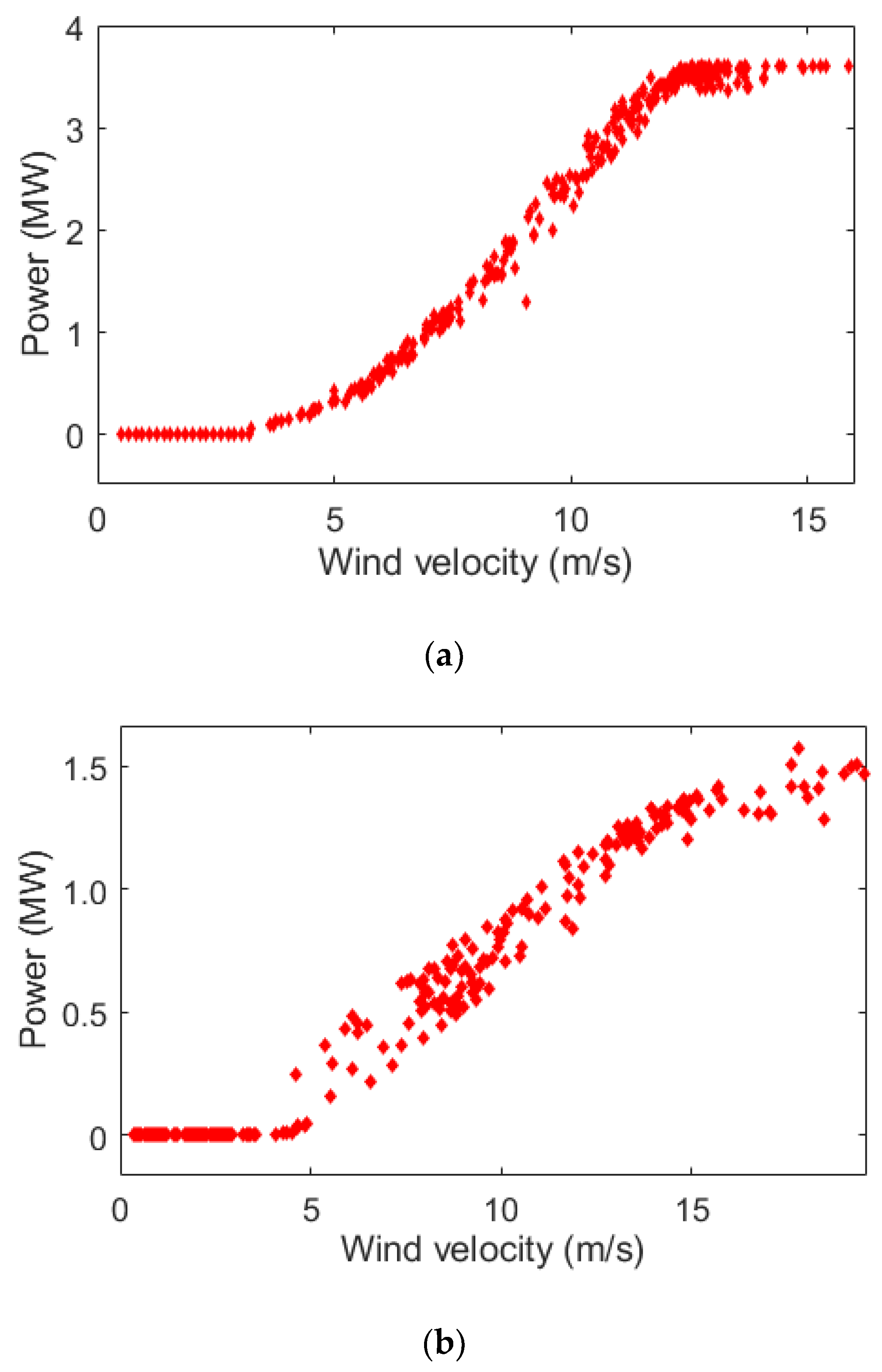
Two WTs are investigated to assess the effectiveness of the proposed SVR approach in identification of the non-parametric MWTP. The investigated WTs are Nordex N117/3600 and Bazán 62/1300, whose power measurements and the corresponding wind velocities are shown in Figure 3. These measurements were recorded in Turkey during 2018 and Spain during 2019, respectively. The numbers of hourly measured data for the two turbines are 265 and 317, respectively. The data cover the full range of wind speeds and turbine powers. The data used were not purified in the compared methods in the literature, so we do the same to compare fairly. Data purification is a suggested topic of research for future work. The WTs specifications are listed in Table 1.
Our findings have been obtained via MATLAB-R2021 under Windows 11 running on a laptop with an Intel Core i7-1065G7 CPU at 1.3 GHz (eight CPUs) with RAM of 16 GB.
For the non-parametric MWTP based on the SVR, three types of kernel function, namely the RBF, linear, and polynomial are tested for choosing the best type according to the RASE. A total of 70% of data is used for training. The hyperparameter is tuned using 5-fold CV for the least square SVR model. The remaining 30% is used for testing. Table 2 reports the tested SVR configurations and their RASEs based on CV for each kernel type.
As revealed in Table 2, the RBF has the smallest RASE, so RBF is selected as the kernel function of the SVR for the non-parametric MWTP.
In this article, the 5-ParLog, 6-ParLog, and MTanh models are employed for the parametric MWTP for comparison with the non-parametric MWTP. For the parametric MWTP, the findings of three evolutionary optimizers [21] and a non-evolutionary optimizer are employed for the comparison with the SVR. The evolutionary optimizers are ASOA, MBA, and ISOA. The maximum number of iterations and the population are 150 and 20, respectively. The non-evolutionary optimizer is LM.
The non-parametric MWTP based on the SVR is compared with the parametric MWTP based on the ASA, MBA, ISA, and LM, according to their findings. The comparison demonstrates that the RASE produced via the SVR is less than that of the ASA, MBA, ISOA, and LM, by 0.4% to 93.8%, as revealed in Table 3 and Table 4. The present dataset exhibits a higher degree of noise and variability, particularly in the nonlinear transition region, which amplifies the benefit of robust generalization capabilities of the SVR.
For Nordex N117/3600, it can be noticed from Table 3 that the best obtained objective value is 0.089663 through the suggested SVR; the LM based on the MTanh model came second, achieving 0.098229, while the LM based on the 5-ParLog model had the worst objective value of 1.396756. For Bazán 62/1300, it can be observed from Table 4 that the best obtained objective value is 0.098871 through the suggested SVR; the ISOA based on the 6-ParLog model came second, achieving 0.099275, while the LM based on the 5-ParLog model had the worst objective value of 1.590634.
The comparison between the non-parametric MWTP based on the SVR and the parametric MWTP based on the ASA, MBA, ISA, and LM according to the average processing time per run is revealed in Table 5 and Table 6, where the average processing times per run of the LM and SVR are much smaller than that of the ASA, MBA, and ISA. However, the objective value of the SVR is smaller than the LM, so the SVR is superior to the LM. This proves that the suggested SVR for the non-parametric MWTP achieves the best objective value, with an acceptable computation time.
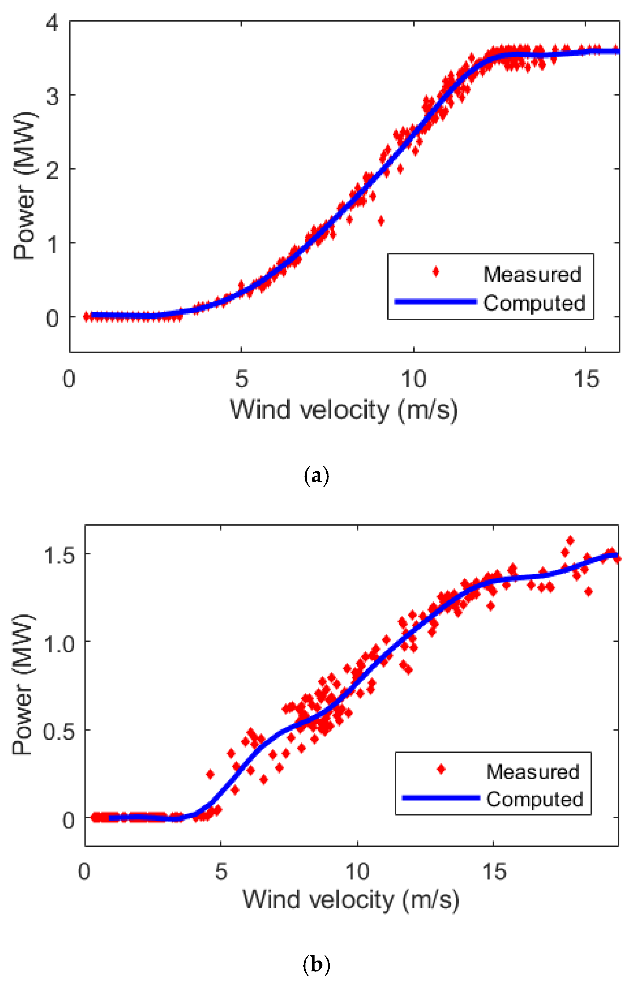
The visual comparison between the calculated power via the non-parametric MWTP based on the SVR and the actual power data is performed. The evaluated P-ν characteristics of WTs via the non-parametric MWTP based on the SVR with the actual data are revealed in Figure 4. The evaluated P-ν curve via the non-parametric MWTP based on the SVR mediates the actual points, which attests to the precision of the extracted non-parametric MWTP.

7.2. Dynamic Wind Force

7.2.1. Parameter Sensitivity Analysis

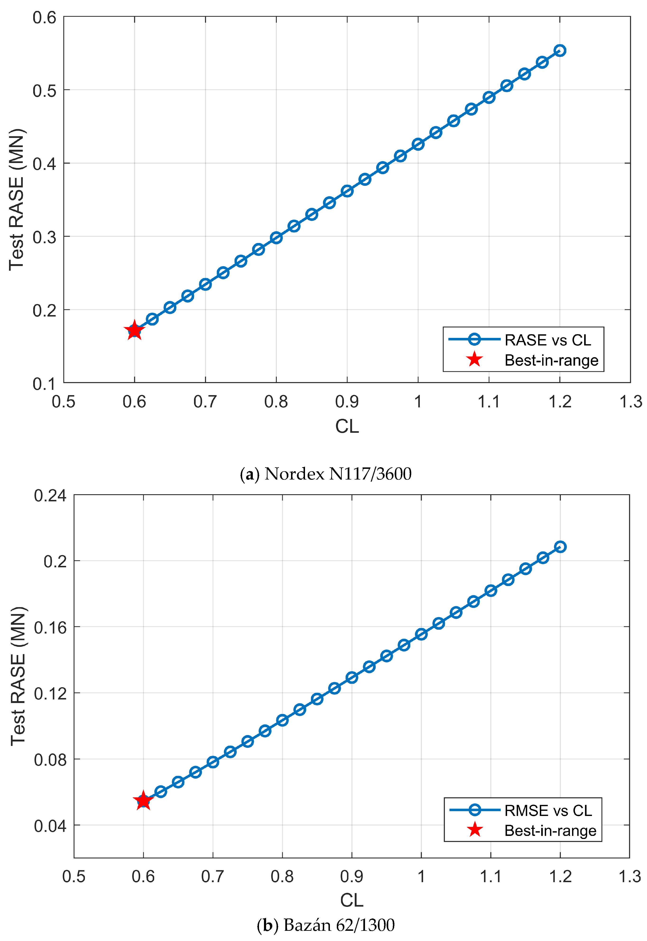
The sole parameter CL is studied, varying it within its nominal range [0.6, 0.12]. Figure 5 shows that changes in CL have a clear monotonic influence on RASE of F, confirming its central role in model accuracy. It is found that CL = 0.6 at the minimum values of RASE, namely 0.171 and 0.055, for Nordex N117/3600 and Bazán 62/1300, respectively.

7.2.2. Analysis of Dynamic Wind Forces

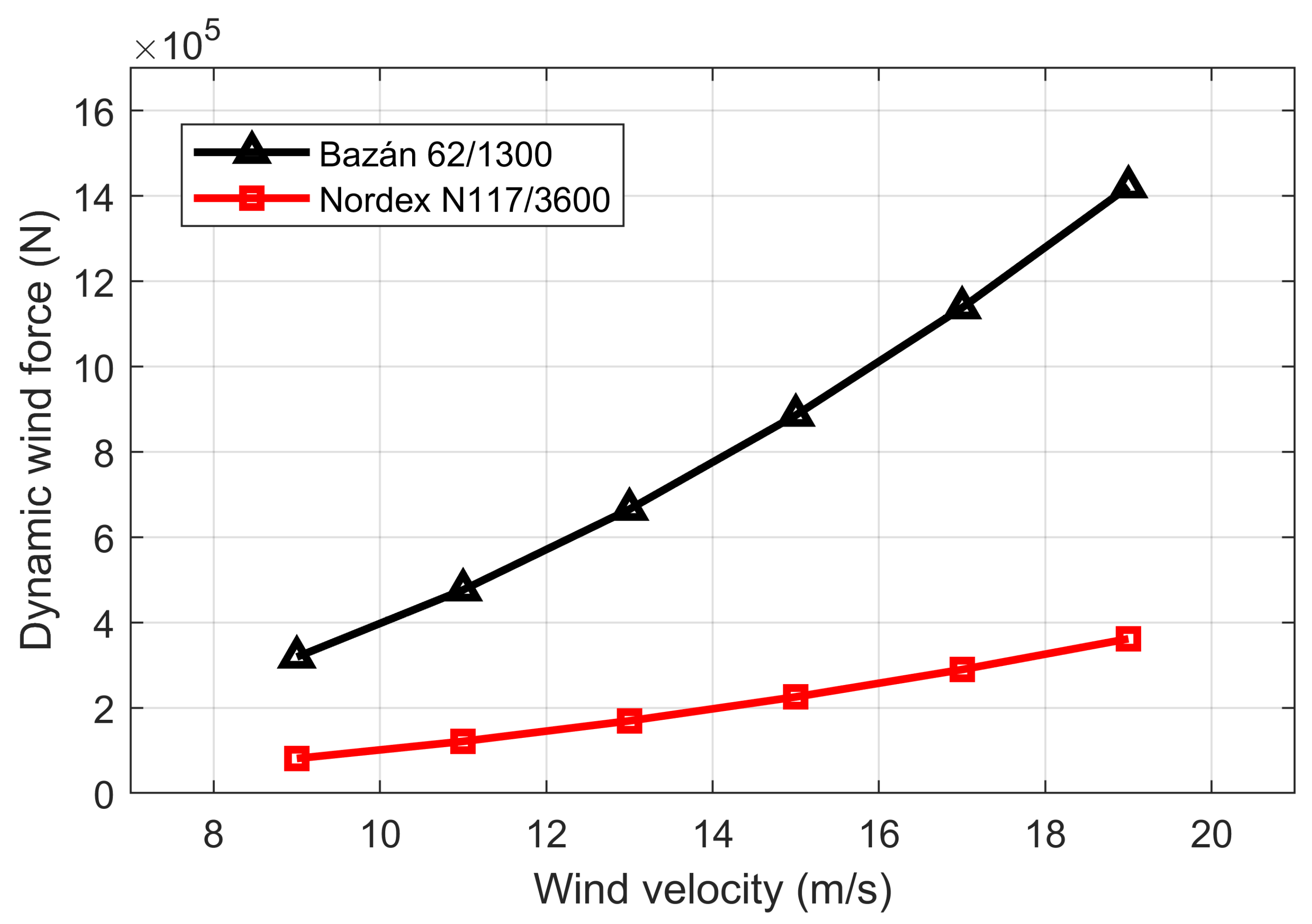
The computed dynamic wind forces (F) on two types of HAWTs, i.e., Nordex N117/3600 and Bazán 62/1300, at several wind velocities of 9, 11, 13, 15, 17, and 19 m/s, are listed in Table 7. The relationship between F and ν is plotted in Figure 6. It can be noted from Figure 6 that the value of F increases when ν increases. This is because the F is directly proportional to the square of ν.
Additionally, the first WT (Nordex N117/3600) exhibits a steep increase in F as ν increases. However, the second WT (Bazán 62/1300) also shows an increasing trend, but at a slower rate compared to Nordex N117/3600. The Bazán 62/1300 experiences a significantly lower F at the same ν. This is because the tower height and rotor diameter of Nordex N117/3600 are larger than that of Bazán 62/1300. This indicates that Nordex N117/3600 is more efficient, resulting in a higher power output.
It is also clear that there is a convergence between the F values at low values of ν, while the F values diverge at high values of ν. This indicates that Nordex N117/3600 is relatively unstable at high speeds. The higher forces acting on Nordex N117/3600 require a more robust structure to withstand these loads.

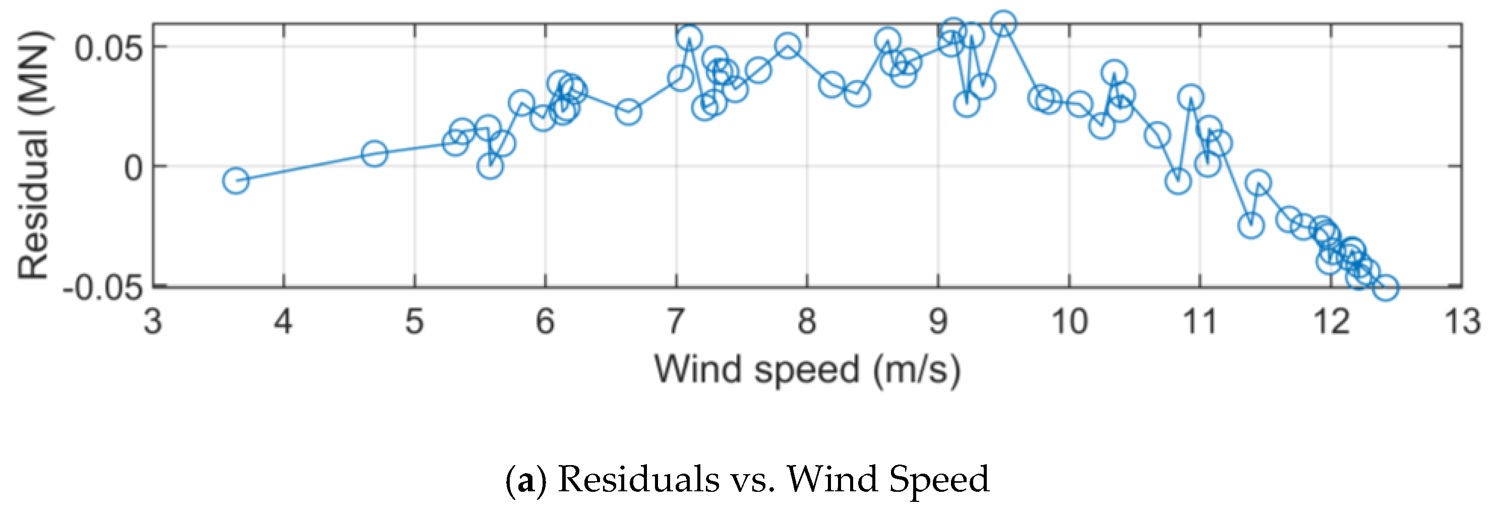
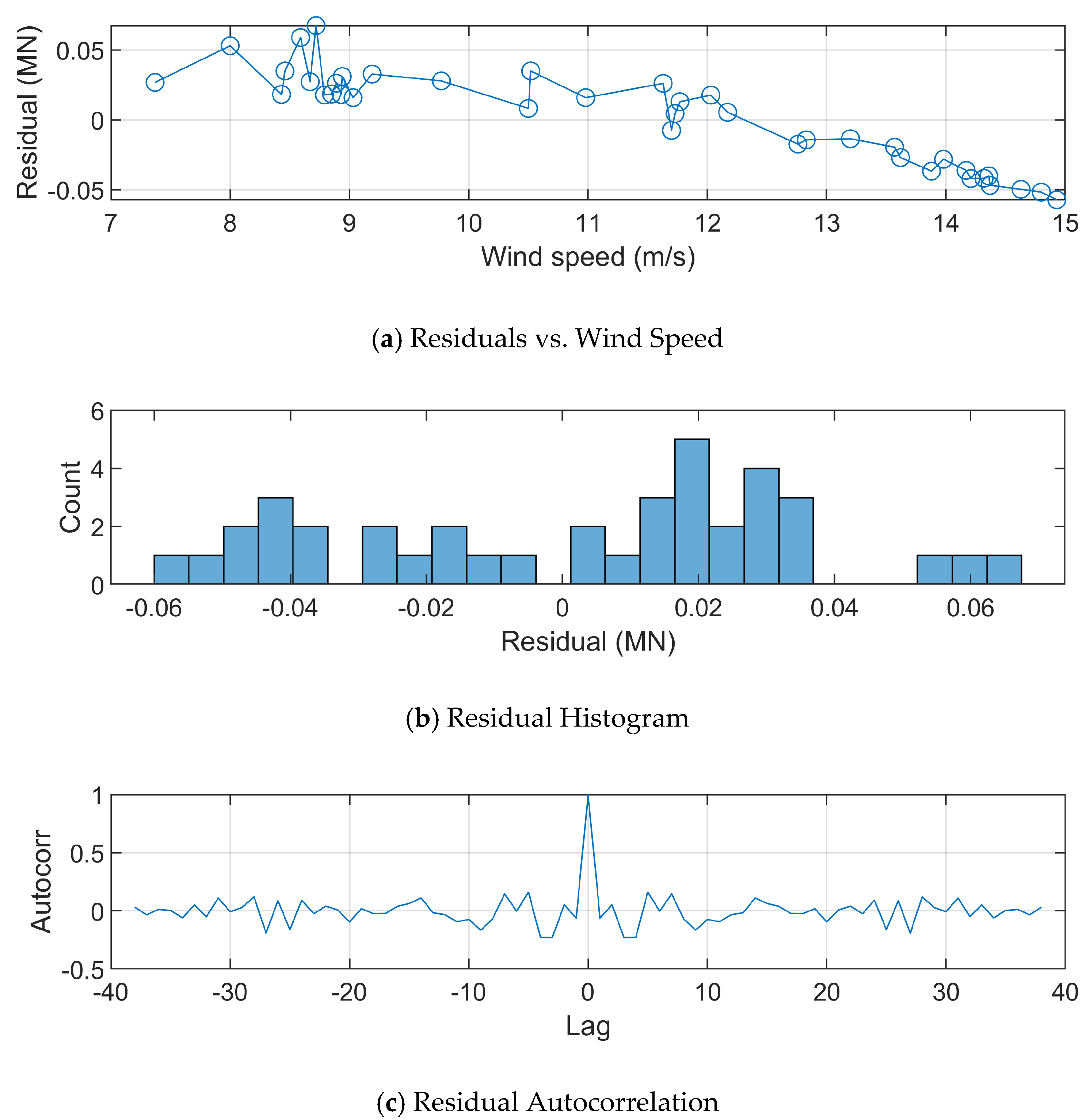
7.2.3. Residual Analysis

The residuals (=observed − predicted) for the dynamic model are analyzed in both time and frequency domains, as revealed in Figure 7 and Figure 8. The results show that the residuals are zero-mean, normally distributed, and free from significant autocorrelation, indicating no systematic bias. The residual statistics confirm the accuracy of results where for Nordex N117/3600, mean = 0.0125 and standard deviation = 0.0314, and for Bazán 62/1300, mean = 0.0017 and standard deviation = 0.0333.

7.2.4. Independent Test Set Validation

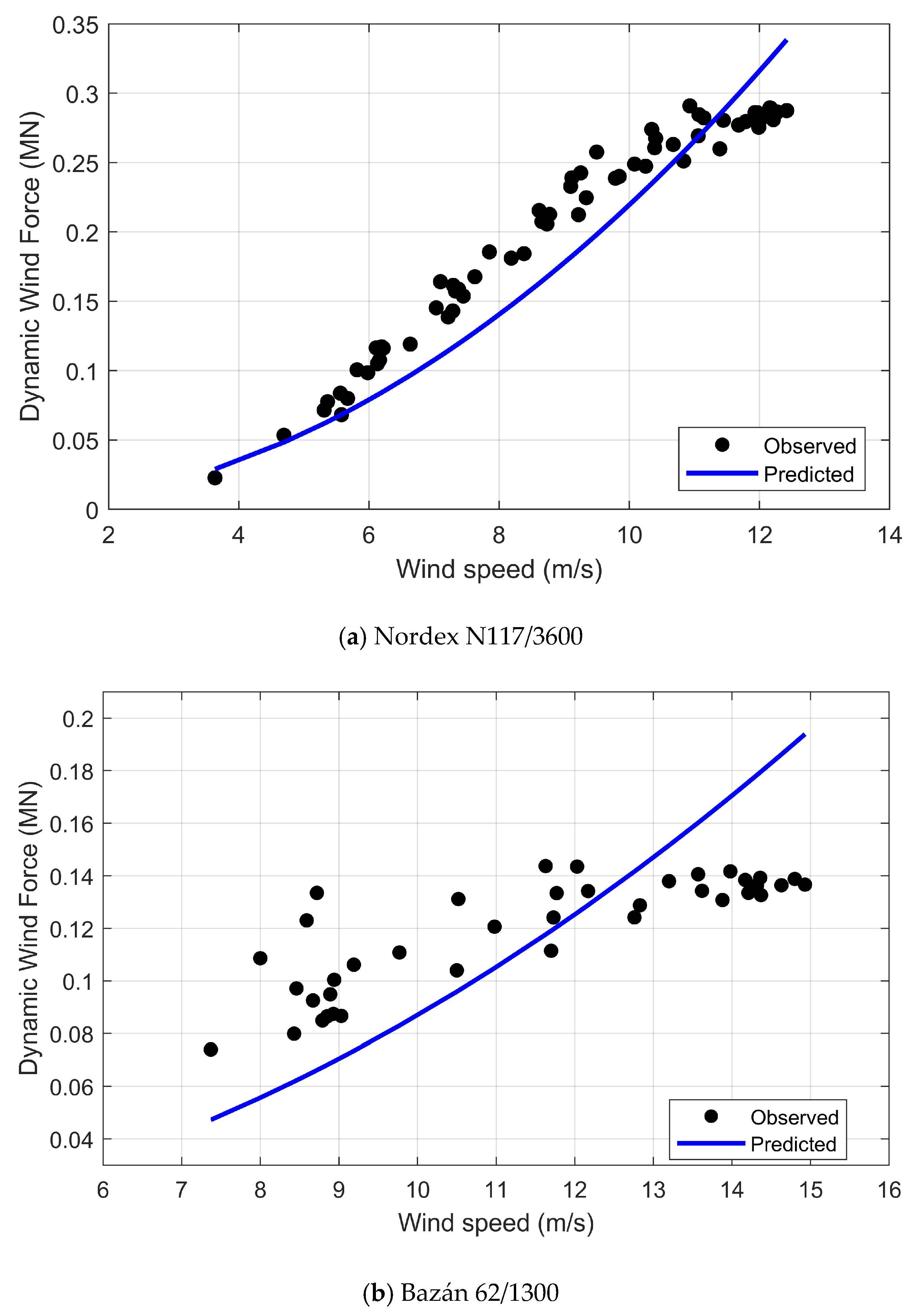
The dynamic dataset was split into 70% training and 30% testing. The test results are revealed in Figure 9, where RASE = 0.034 and 0.033 MN for Nordex N117/3600 and Bazán 62/1300, respectively. These values closely match training performance, where RASE = 0.029 and 0.039 MN, respectively, confirming the generalization capability.

7.3. Eigen Parameter Analysis

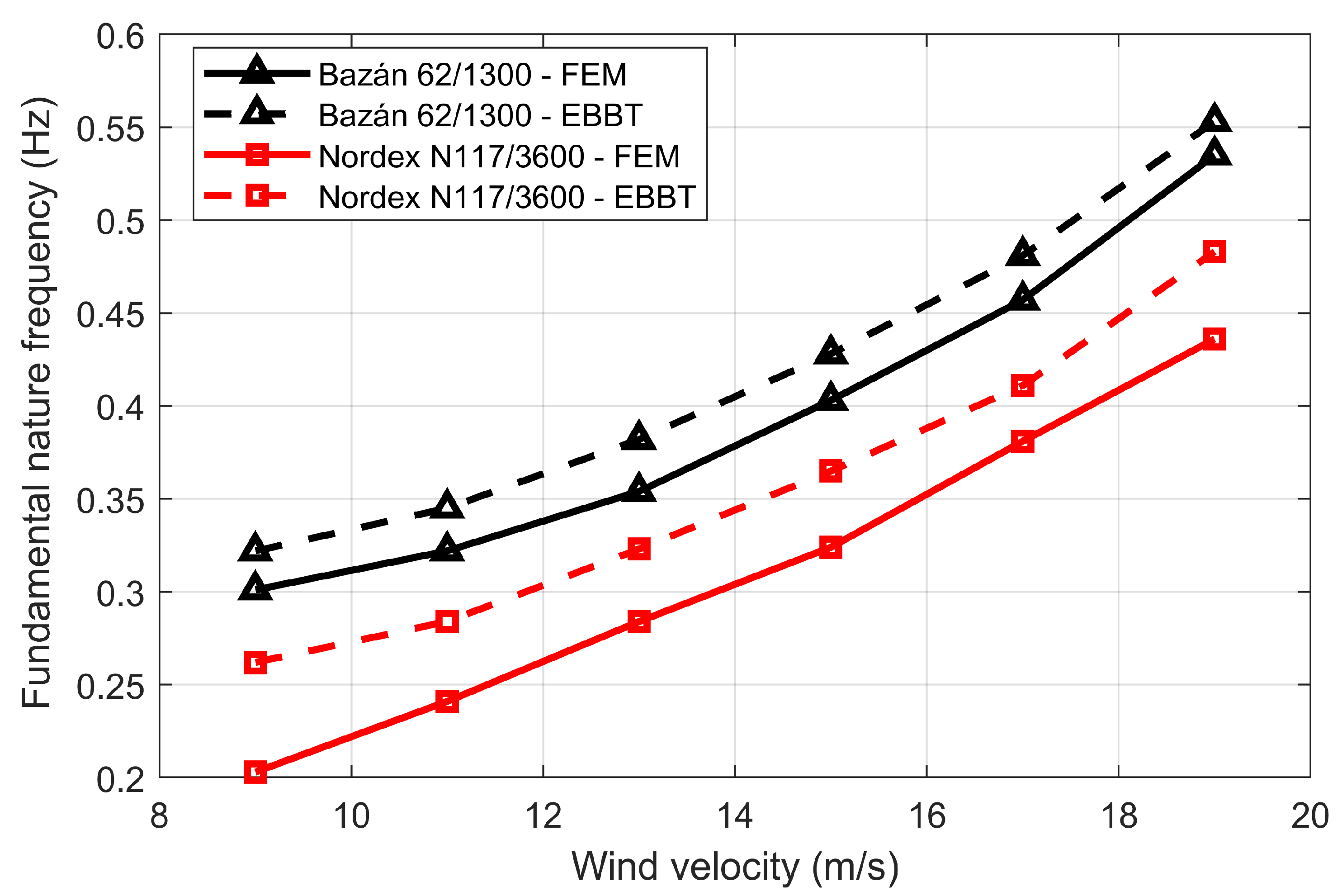
Two numerical methods, namely FEM and EBBT, are used for calculating the fundamental fn at several wind velocities for the two studied WTs, as listed in Table 8. The relationship between fn and ν is shown in Figure 10. It can be observed from Figure 10 that the fn values of Bazán 62/1300 are higher than that of Nordex N117/3600 by about 18.83%. This is because the elastic flexural modulus and the stiffness of Bazán 62/1300 are higher than those of Nordex N117/3600.
Figure 10 shows that fn reaches its peak at ν of 19 m/s, whereas at ν of 9 m/s, a low fn is obtained. This means that when ν increases, the aerodynamic forces acting on the blades increase. These forces increase the strain on the blades, just as tightening a string increases its vibration frequency. This stress increases structural rigidity and raises the WT intrinsic frequency. The value of fn rises on average by around 46.17% when ν increases from 9 m/s to 19 m/s.
It can be also noticed from Figure 10 that there is a near-constant convergence between fn values of the two WTs at ν values of 9, 11, 13, and 15 m/s, while at ν values of 17 and 19 m/s, there is a divergence in the fn values. This is because at moderate values of ν (9–15 m/s), both WTs may operate in a similar aerodynamic regime, where the blade pitch angles are relatively stable, the rotor speeds are within a controlled range, and the structural deformations are minimal. These conditions lead to similar effective stiffness changes, causing fn to rise at a comparable rate.
At higher values of ν (17–19 m/s), the WTs often enter different operational modes. Bazán 62/1300 may experience greater aerodynamic or centrifugal stiffening, increasing its fn more sharply. Nordex N117/3600 may engage pitch control or power limiting strategies, which can reduce the increase rate of fn.
It can be also noted from Table 8 that at lower values of ν, namely 9 m/s, the values of fn computed via the FEM for both WTs are 0.203 Hz and 0.301 Hz, which are lower than those computed via the EBBT (0.262 Hz and 0.322 Hz). This pattern continues at higher values of ν, indicating that the FEM tends to predict a lower fn compared to the EBBT across the range of values tested. The differences between the two techniques widen as ν increases, indicating that the choice of numerical method may significantly affect fn predictions.
The comparison of fn vs. ν, as shown in Figure 10, is a valuable tool for engineers and designers in the wind energy sector. It highlights the importance of tailoring WT design to expect the wind conditions and ensures that the fn is well-separated from the excitation frequencies. The clear distinction between the two models also underscores the diversity in the WT engineering approaches.
The modern WTs use pitch control and torque control to optimize performance. These systems can alter the dynamic behavior of the WT, especially under varying ν, affecting fn.

8. Conclusions

In this paper, the novel application of the SVR to identify the non-parametric MWTP has been treated. The objective of establishing an accurate MWTP is to precisely forecast and manage the wind energy throughout the numerous wind velocities. The F f i t aims at minimizing the RASE between the calculated and associated recoded wind power values of the WT. The proposed MWTP efficacy has been assessed through comparing its computed power values with the actual power values of a pair of WTs. The computed power values are agreeable with the actual power values in both case studies. Furthermore, a comparison between the SVR-based findings and findings of other approaches has been performed. The SVR-based findings show that the RASE has been reduced by 0.4% to 93.8% from other approaches, and this manifests the great superiority of the SVR over other approaches. Additionally, the smallness of the average processing time per run of the suggested SVR for the non-parametric MWTP has proved that the computation cost is much smaller than that of most of compared approaches. The close agreement between the FEM and the EBBT at lower wind velocities indicates that EBBT may be sufficient for the preliminary analysis, but the FEM is preferable for detailed designs. Lower natural frequencies at higher wind speeds could lead to resonance issues if they approach the excitation frequencies from the wind or the rotor harmonics. Accurate modeling using the FEM is crucial for predicting the dynamic behavior, especially for the flexible structures like Bazán 62/1300. The fn values of Bazán 62/1300 are higher than that of Nordex N117/3600 by about 18.83%. This is because the elastic flexural modulus and the stiffness of Bazán 62/1300 are higher than those of Nordex N117/3600. The proposed future work involves filtration of the recorded measurements of the WT and dynamic effects such as wind velocity fluctuations and intermittent operation using time-series data from variable wind profiles.

Author Contributions

Conceptualization, A.M.A. and M.I.E.; methodology, A.M.A. and M.I.E.; software, A.M.A. and M.I.E.; validation, A.M.A. and M.I.E.; formal analysis, A.M.A. and M.I.E.; investigation, A.M.A. and M.I.E.; resources, A.M.A. and M.I.E.; data curation, A.M.A. and M.I.E.; writing—original draft preparation, A.M.A. and M.I.E.; writing—review and editing, A.M.A. and M.I.E.; visualization, A.M.A. and M.I.E.; supervision, A.M.A. and M.I.E.; project administration, A.M.A. and M.I.E.; funding acquisition, A.M.A. and M.I.E. All authors have read and agreed to the published version of the manuscript.

Funding

This research was funded by the Deanship of Scientific Research at Northern Border University, Arar, KSA, through the project number “NBU-FFR-2025-2968-02”.

Data Availability Statement

The data that support the findings of this study are available from the corresponding author upon reasonable request.

Acknowledgments

The authors extend their appreciation to the Deanship of Scientific Research at Northern Border University, Arar, KSA, for funding this research work through project number “NBU-FFR-2025-2968-02”.

Conflicts of Interest

The authors confirm that there are no conflicts of interest.

References

  1. Kariman, H.; Hosseinzadeh, S.; Khiadani, M.; Nazarieh, M. 3D-CFD analysing of tidal Hunter turbine to enhance the power coefficient by changing the stroke angle of blades and incorporation of winglets. Ocean Eng. 2023, 287, 115713. [Google Scholar] [CrossRef]
  2. Aranizadeh, A.; Mirmozaffari, M.; Farahani, B.K. Maximizing Wind Turbine Power Generation Through Adaptive Fuzzy Logic Control for Optimal Efficiency and Performance. Wind 2025, 5, 4. [Google Scholar] [CrossRef]
  3. Dias, F.L.; Naik, A.J. A Novel Approach to Wavelet Neural Network-Based Wind Power Forecasting. Wind 2025, 5, 14. [Google Scholar] [CrossRef]
  4. Letzgus, S.; Müller, K.-R. An explainable AI framework for robust and transparent data-driven wind turbine power curve models. Energy AI 2023, 15, 100328. [Google Scholar] [CrossRef]
  5. Goudarzi, A.; Davidson, I.E.; Ahmadi, A.; Venayagamoorthy, G.K. Intelligent Analysis of Wind Turbine Power Curve Models. In Proceedings of the IEEE Symposium on Computational Intelligence Applications in Smart Grid (CIASG), Orlando, FL, USA, 9–12 December 2014; pp. 1–7. [Google Scholar]
  6. Lydia, M.; Selvakumar, A.I.; Kumar, S.S.; Kumar, G.E.P. Advanced Algorithms for Wind Turbine Power Curve Modeling. IEEE Trans. Sustain. Energy 2013, 4, 827–835. [Google Scholar] [CrossRef]
  7. Yesilbudak, M. Assessment of Power Curve Fitting Performance of Parametric Models for Wind Turbines. Int. J. Renew. Energy Res. 2025, 15, 22–29. [Google Scholar]
  8. Bao, Y.; Yang, Q.; Sun, Y. Iterative Modeling of Wind Turbine Power Curve Based on Least-Square B-Spline Approximation. Asian J. Control 2019, 21, 2004–2016. [Google Scholar] [CrossRef]
  9. Fu, Z.-Y.; Lin, G.-Q.; Tian, W.-D.; Pan, Z.-H.; Zhang, W.-C. Novel nonlinear wind power prediction based on improved iterative algorithm. Syst. Sci. Control. Eng. 2025, 13, 1. [Google Scholar] [CrossRef]
  10. Kusiak, A.; Zheng, H.; Song, Z. Models for Monitoring Wind Farm Power. Renew. Energy 2009, 34, 583–590. [Google Scholar] [CrossRef]
  11. Seo, S.; Oh, S.; Kwak, H. Wind Turbine Power Curve Modeling Using Maximum Likelihood Estimation Method. Renew. Energy 2019, 136, 1164–1169. [Google Scholar] [CrossRef]
  12. Goudarzi, A.; Swanson, A.G.; Kazemi, M.; Wang, K. Intelligent wind turbine power curve modelling using the third version of cultural algorithm (CA3). Int. J. Renew. Energy Res. 2017, 7, 1340–1351. [Google Scholar] [CrossRef]
  13. Yesilbudak, M.; Ozcan, A. Performance Comparison of Metaheuristic Optimization-Based Parametric Methods in Wind Turbine Power Curve Modeling. IEEE Access 2024, 12, 99372–99381. [Google Scholar] [CrossRef]
  14. Jin, R.; Wang, L.; Huang, C.; Jiang, S. Wind Turbine Generation Performance Monitoring with Jaya Algorithm. Int. J. Energy Res. 2019, 43, 1604–1611. [Google Scholar] [CrossRef]
  15. Marčiukaitis, M.; Žutautaitė, I.; Martišauskas, L.; Jokšas, B.; Gecevičius, G.; Sfetsos, A. Non-Linear Regression Model for Wind Turbine Power Curve. Renew. Energy 2017, 113, 732–741. [Google Scholar] [CrossRef]
  16. Tao, S.; Xu, Q.; Feijóo, A.; Kuenzel, S.; Bokde, N. Integrated Wind Farm Power Curve and Power Curve Distribution Function Considering the Wake Effect and Terrain Gradient. Energies 2019, 12, 2482. [Google Scholar] [CrossRef]
  17. Yesilbudak, M. A Novel Power Curve Modeling Framework for Wind Turbines. Adv. Electr. Comput. Eng. 2019, 19, 29–40. [Google Scholar] [CrossRef]
  18. Rose, J.; Hiskens, I.A. Estimating Wind Turbine Parameters and Quantifying Their Effects on Dynamic Behavior. In Proceedings of the IEEE Power and Energy Society General Meeting—Conversion and Delivery of Electrical Energy in the 21st Century, Pittsburgh, PA, USA, 20–24 July 2008; pp. 1–7. [Google Scholar]
  19. Krishna, J.; Bhargava, V.; Donepudi, J. BEM Prediction of Wind Turbine Operation and Performance. Int. J. Renew. Energy Res. 2018, 8, 1962–1973. [Google Scholar]
  20. Agwa, A.M. Interior Search Optimization Algorithm for Modeling Power Curve of Wind Turbine. Int. J. Renew. Energy Res. 2020, 10, 1349–1358. [Google Scholar] [CrossRef]
  21. Wang, Y.; Duan, X.; Zou, R.; Zhang, F.; Li, Y.; Hu, Q. A novel data-driven deep learning approach for wind turbine power curve modeling. Energy 2023, 270, 126908. [Google Scholar] [CrossRef]
  22. Caro, F.D.; Vaccaro, A.; Villacci, D. Adaptive Wind Generation Modeling by Fuzzy Clustering of Experimental Data. Electronics 2018, 7, 47. [Google Scholar] [CrossRef]
  23. Cao, Y.; Hu, Q.; Shi, H.; Zhang, Y. Prediction of Wind Power Generation Base on Neural Network in Consideration of the Fault Time. IEEJ Trans. Electr. Electron. Eng. 2019, 14, 670–679. [Google Scholar] [CrossRef]
  24. Demirdelen, T.; Tekin, P.; Aksu, I.O.; Ekinci, F. The Prediction Model of Characteristics for Wind Turbines Based on Meteorological Properties Using Neural Network Swarm Intelligence. Sustainability 2019, 11, 4803. [Google Scholar] [CrossRef]
  25. Bai, L.; Crisostomi, E.; Raugi, M.; Tucci, M. Wind Turbine Power Curve Estimation Based on Earth Mover Distance and Artificial Neural Networks. IET Renew. Power Gener. 2019, 13, 2939–2946. [Google Scholar] [CrossRef]
  26. Mushtaq, K.; Waris, M.; Zou, R.; Shafique, U.; Khan, N.; Khan, M.; Jameel, M.; Khan, M.I. A Comprehensive Approach to Wind Turbine Power Curve Modeling: Addressing Outliers and Enhancing Accuracy. Energy 2024, 304, 131981. [Google Scholar] [CrossRef]
  27. Bilal, B.; Adjallah, K.; Sava, A.; Ouassaid, M. Wind turbine output power prediction and optimization based on a novel adaptive neuro-fuzzy inference system with the moving window. Energy 2023, 263, 126159. [Google Scholar] [CrossRef]
  28. Pandit, R.K.; Infield, D. Comparative Analysis of Gaussian Process Power Curve Models Based on Different Stationary Covariance Functions for The Purpose of Improving Model Accuracy. Renew. Energy 2019, 140, 190–202. [Google Scholar] [CrossRef]
  29. Mehrjoo, M.; Jozani, M.J.; Pawlak, M. Wind Turbine Power Curve Modeling for Reliable Power Prediction Using Monotonic Regression. Renew. Energy 2020, 147, 214–222. [Google Scholar] [CrossRef]
  30. He, C.; Peng, J.; Jiang, W.; Wang, C.; Li, J.; Tan, Z. A hybrid time series analysis-genetic algorithm-support vector machine model for enhanced landslide prediction. Int. J. Ind. Eng. Comput. 2025, 16, 785–798. [Google Scholar] [CrossRef]
  31. Xiao, J.; Liu, G.; Huang, M.; Yin, Z.; Gao, Z. A kernel-free L1 norm regularized ν-support vector machine model with application. Int. J. Ind. Eng. Comput. 2023, 14, 691–706. [Google Scholar] [CrossRef]
  32. Hosseini, M.S.; Karimi, A. Meta-Heuristic Enhanced SVR for Pile-Bearing Capacity Estimation. Int. J. Geotech. Eng. 2024, 15, 1234–1247. [Google Scholar]
  33. Wang, J.P.; Liu, Y. Novel Support Vector Regression Approach for Equipment Health Monitoring. Comput. Intell. Neurosci. 2021, 2021, 6675078. [Google Scholar]
  34. Li, X.; Wang, J.; Zhang, H. Combining SVR with genetic algorithms for equipment fault detection. J. Mach. Cond. Monit. 2021, 27, 357–367. [Google Scholar]
  35. Luo, J.; Hong, T.; Gao, Z.; Fang, S. A Robust Support Vector Regression Model for Electric Load Forecasting. Int. J. Forecast. 2023, 39, 1005–1020. [Google Scholar] [CrossRef]
  36. Zhang, Z.; Zhang, Q.; Liang, H.; Gorbani, B. Optimizing Electric Load Forecasting with Support Vector Regression/LSTM Optimized by Flexible Gorilla Troops Algorithm and Neural Networks A Case Study. Sci. Rep. 2024, 14, 22092. [Google Scholar] [CrossRef]
  37. Verma, R.; Tiwari, S. Improving Offshore Wind Farm Power Prediction with Enhanced SVR Models. J. Energy Eng. 2023, 149, 105–114. [Google Scholar]
  38. Chen, L.; Wang, X.; Zhang, Y. Support Vector Regression for Solar Power System Forecasting with Climatic Data. IEEE Trans. Sustain. Energy 2023, 14, 102–109. [Google Scholar]
  39. Lee, D.; Chang, K.; Oh, H. Application of SVR for Smart Renewable Energy System Forecasting. IEEE Access 2024, 11, 15050–15061. [Google Scholar]
  40. Gupta, A.; Mehta, P.; Sharma, K. Optimized SVR for Forecasting Renewable Energy Outputs Using Metaheuristics. Energy Rep. 2023, 8, 1021–1032. [Google Scholar]
  41. Chandrakala, K.; Rajan, P. A Hybrid Machine Learning Approach for Price Forecasting in Electricity Market with Smart Bidding Strategies and Wind Energy Influence. Int. Rev. Model. Simul. (IREMOS) 2022, 15, 414–424. [Google Scholar] [CrossRef]
  42. Park, T.J.; Lee, J.K.; Choi, H. Real-Time Dynamic System Modeling in Robotics Using SVR. IEEE Trans. Robot. 2023, 39, 254–266. [Google Scholar]
  43. Yeganeh, A.; Abbasi, S.A.; Shongwe, S.C.; Malela-Majika, J.-C.; Shadman, A.R. An Evolutionary SVR Model for Monitoring Poisson Profiles in Manufacturing. Soft Comput. 2023, 27, 6789–6799. [Google Scholar]
  44. Das, P.K.; Gupta, S.K. Evolutionary SVR Model for Poisson Profiles in Pollution Monitoring. Soft Comput. 2023, 27, 8954–8966. [Google Scholar]
  45. Zhang, H.; Xu, L.; Wei, P. Enhancing Image Resolution With SVR. IEEE Trans. Image Process. 2023, 32, 1456–1467. [Google Scholar]
  46. Singh, R.K.; Verma, P.; Tripathi, S. Advancements in SVR for Healthcare Applications: A Review. Information 2023, 15, 235–248. [Google Scholar]
  47. Shoko, C.; Sigauke, C. Short-Term Forecasting of COVID-19 Using Support Vector Regression: An Application Using Zimbabwean Data. Am. J. Infect. Control 2023, 51, 1095–1107. [Google Scholar] [CrossRef]
  48. Fang, Y. Stock Price Forecasting Based on Improved Support Vector Regression. In Proceedings of the 2020 7th International Conference on Information Science and Control Engineering (ICISCE), Changsha, China, 18–20 December 2020; pp. 1351–1354. [Google Scholar]
  49. Lee, P.L.; Kim, J.H. Predicting Customer Behavior Using Support Vector Regression. Mark. Sci. 2023, 41, 123–134. [Google Scholar]
  50. Villanueva, D.; Feijóo, A.E. Reformulation of Parameters of The Logistic Function Applied to Power Curves of Wind Turbines. Electr. Power Syst. Res. 2016, 137, 51–58. [Google Scholar] [CrossRef]
  51. Villanueva, D.; Feijóo, A. Comparison of Logistic Functions for Modeling Wind Turbine Power Curves. Electr. Power Syst. Res. 2018, 155, 281–288. [Google Scholar] [CrossRef]
  52. Wang, Y.; Hu, Q.; Li, L.; Foley, A.M.; Srinivasan, D. Approaches to Wind Power Curve Modeling: A Review and Discussion. Renew. Sustain. Energy Rev. 2019, 116, 109422. [Google Scholar] [CrossRef]
  53. Manwell, J.F.; McGowan, J.G.; Rogers, A.L. Wind Energy Explained: Theory, Design and Application; John Wiley & Sons: Hoboken, NJ, USA, 2010. [Google Scholar]
  54. Burton, T.; Jenkins, N.; Sharpe, D.; Bossanyi, E. Wind Energy Handbook; John Wiley & Sons: Hoboken, NJ, USA, 2011. [Google Scholar]
  55. Wan, J.-H.; Bai, R.; Li, X.-Y.; Liu, S.-W. Natural Frequency Analysis of Monopile Supported Offshore Wind Turbines Using Unified Beam-Column Element Model. J. Mar. Sci. Eng. 2023, 11, 628. [Google Scholar] [CrossRef]
  56. Li, X.Y.; Wan, J.H.; Zhao, H.P.; Liu, S.W. Three-Dimensional analysis of nonlinear pile–soil interaction responses using 3D pile element model. Int. J. Geomech. 2021, 21, 04021129. [Google Scholar] [CrossRef]
  57. Tong, W. Wind Power Generation and Wind Turbine Design; WIT Press: Southampton, UK, 2010. [Google Scholar]
  58. Rao, S.S.; Yap, F.F. Mechanical Vibrations; Addison-Wesley: New York, NY, USA, 1995. [Google Scholar]
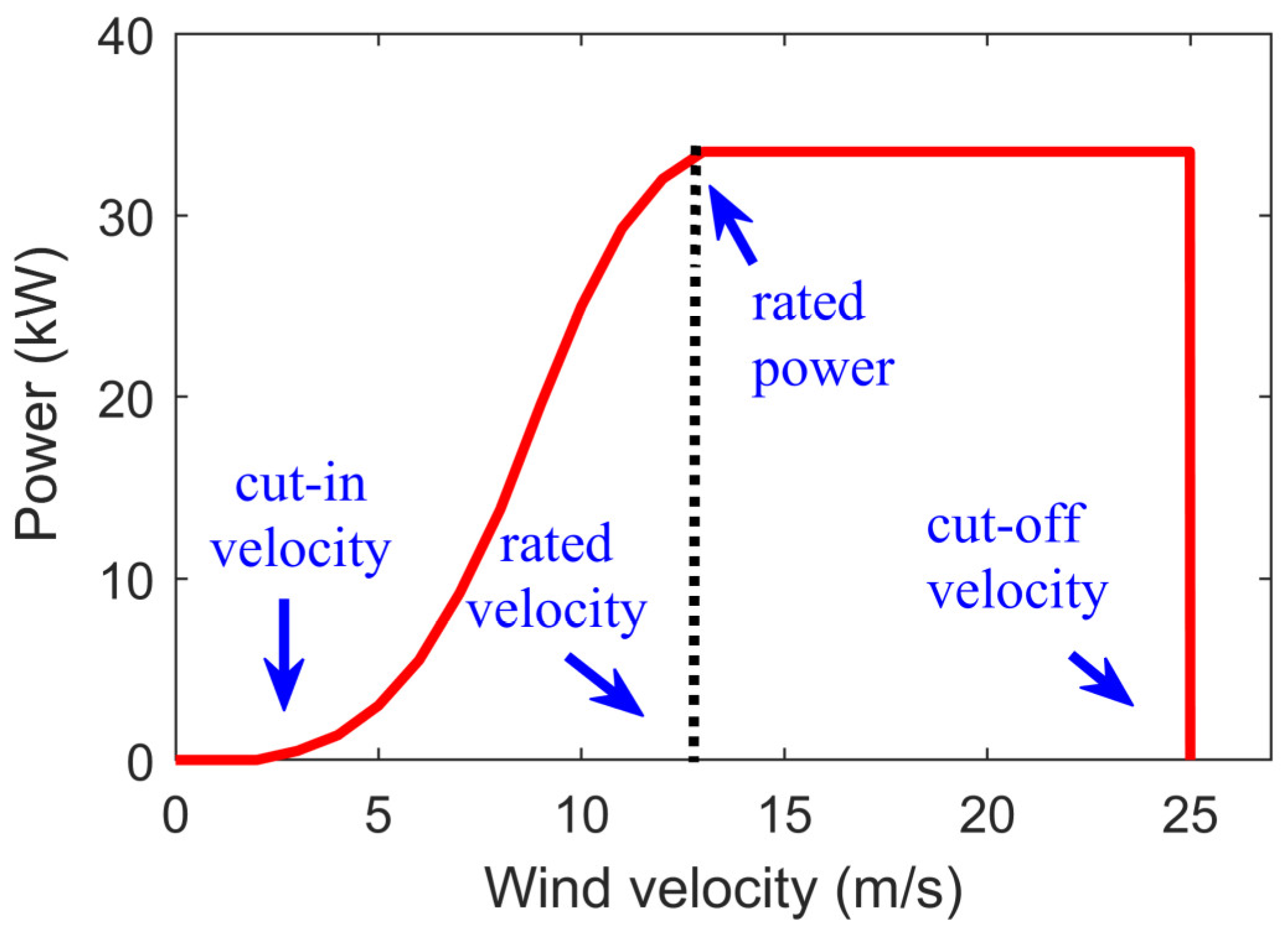
Figure 1. The WT power curve.
Wind 05 00020 g001
Figure 2. Finite element model of HAWT.
Wind 05 00020 g002
Figure 3. P-ν measurements of (a) Nordex N117/3600 and (b) Bazán 62/1300.
Wind 05 00020 g003
Figure 4. P-ν characteristics of non-parametric MWTP based on SVR of (a) Nordex N117/3600 and (b) Bazán 62/1300.
Wind 05 00020 g004
Figure 5. Sensitivity of RASE to CL within its nominal range [0.6, 1.2].
Wind 05 00020 g005
Figure 6. The relationship between the dynamic wind force and the wind velocity.
Wind 05 00020 g006
Figure 7. Residual analysis of Nordex N117/3600.
Wind 05 00020 g007aWind 05 00020 g007b
Figure 8. Residual analysis of Bazán 62/1300.
Wind 05 00020 g008
Figure 9. Observed vs predicted force (test results).
Wind 05 00020 g009
Figure 10. Comparison of fn vs. ν using FEM and EBBT for Nordex N117/3600 and Bazán 62/1300.
Wind 05 00020 g010
Table 1. WT specifications.
ModelNordex N117/3600Bazán 62/1300
P n   ( M W ) 3.61.3
ν n   ( m / s ) 1315
ν c i n   ( m / s ) 33
ν c o f f   ( m / s ) 2525
H   ( m ) 7650
D   ( m ) 116.862
F r e q u e n c y   ( H z ) 5050
V o l t a g e   ( V ) 660690
Table 2. Summary of SVR hyperparameters and CV performance.
Kernel TypeTested Values of C Tested Values of Kernel Bandwidth (γ) Tested Values of ε Best
Parameters Found
Best RASE
Nordex N117/3600Bazán 62/1300
RBF1, 10, 100, 1000, 10,000, 100,0000.001, 0.01, 0.1, 10.001, 0.01, 0.1C = 100, γ = 0.1,
ε = 0.01
0.0896630.098871
Linear1, 10, 100, 1000, 10,000, 100,0000.001, 0.01, 0.1C = 100,
ε = 0.01
0.3003410.168406
Polynomial1, 10, 100, 1000, 10,000, 100,000γ = 0.001, 0.01, 0.1, 1
degree = 2, 3, 4
0.001, 0.01, 0.1C = 100, γ = 0.1,
degree = 3,
ε = 0.01
0.1608750.147320
Table 3. The RASE (MW) of Nordex N117/3600.
The Parametric MWTP Model
5-ParLog6-ParLogMTanh
ASA [21]0.2024820.1645420.379188
MBA [21]0.1271020.1212360.193832
ISOA [21]0.0997760.0992750.129178
LM1.3967560.1221460.098229
The Non-Parametric MWTPSVR0.089663
Table 4. The RASE (MW) of Bazán 62/1300.
The Parametric MWTP Model
5-ParLog6-ParLogMTanh
ASA [21]0.1776360.1645420.379188
MBA [21]0.1538910.1212360.193832
ISOA [21]0.1129800.0992750.129178
LM1.5906340.1289060.104787
The Non-Parametric MWTPSVR0.098871
Table 5. The average processing time per run (s) of Nordex N117/3600.
Parametric MWTPModel5-ParLog6-ParLogMTanh
ASA55.3355.7056.96
MBA68.2762.7767.81
ISOA69.0463.7161.49
LM0.020.050.11
Non-Parametric MWTPSVR0.27
Table 6. The average processing time per run (s) of Bazán 62/1300.
Parametric MWTPModel5-ParLog6-ParLogMTanh
ASA48.9946.5050.99
MBA66.6966.3378.11
ISOA56.5249.9453.01
LM0.060.050.09
Non-Parametric MWTPSVR0.23
Table 7. Dynamic wind force at various wind velocities.
ν (m/s)F (N)
Nordex N117/3600Bazán 62/1300
9318,958.781,184.1
11476,469.3121,275
13665,481.9169,384.1
15885,996.5225,511.4
171,138,013.4289,656.8
191,421,532.3361,820.5
Table 8. The fundamental fn in Hz at various values of ν using FEM and EBBT.
ν (m/s)Fundamental fn (Hz)
FEMEBBT
Nordex N117/3600Bazán 62/1300Nordex N117/3600Bazán 62/1300
90.2030.3010.2620.322
110.2410.3220.2840.345
130.2840.3540.3230.382
150.3240.4030.3650.428
170.3810.4570.4110.481
190.4360.5350.4830.553
Disclaimer/Publisher’s Note: The statements, opinions and data contained in all publications are solely those of the individual author(s) and contributor(s) and not of MDPI and/or the editor(s). MDPI and/or the editor(s) disclaim responsibility for any injury to people or property resulting from any ideas, methods, instructions or products referred to in the content.