Abstract
The estimation of the aerodynamic characteristics of a rough surface (zero displacement plane and aerodynamic roughness length ) is important in the simulation of atmospheric boundary layer wind in a wind tunnel, since they are parameters involved in various problems of meteorological and wind engineering activities. In this study, morphometric methods were used to present parameterizations of and as functions of roughness and areal density based on wind tunnel measurements of airflow over a rough surface. Vertical profiles of mean wind speed, turbulence intensity, boundary layer depth, and spectral density functions are presented.
1. Introduction
To solve engineering problems such as predicting wind loads on civil structures, the possible interaction between the wind and the structures, the effect of wind on pedestrians, dispersion of air pollutants, etc., it is necessary to simulate the atmospheric boundary layer (ABL) either in a boundary layer wind tunnel or by means of a computational fluid dynamics (CFD) numerical model. However, accurately describing the details of wind speed is somewhat challenging, as wind in the ABL is a turbulent phenomenon. The air velocity is constant over neither time nor space, and its mathematical representation is complex, making a deterministic description difficult.
Synoptic-scale winds exhibit a harmonic content characterized by two peaks: one at the macrometeorological scale and the other at the micrometeorological scale. These peaks are separated by a spectral gap corresponding to time intervals ranging from 10 min to 1 h [1]. In the field of wind engineering, wind speed has traditionally been considered as the sum of a constant mean component, associated with the macrometeorological peak, and a time-varying turbulent fluctuation, corresponding to the micrometeorological peak. The latter is modeled as a stationary Gaussian random process [2,3]. This approach assumes that strong winds follow a stationary stochastic process and that the turbulent characteristics of the wind, such as turbulence intensity, integral turbulence scale, and power spectral density (PSD), remain constant and time-independent.
Recent studies have revealed that strong winds, particularly those associated with non-synoptic phenomena such as thunderstorm winds (especially downburst) and tornadoes, exhibit significant characteristics that vary over time [4]. These include not only changes in mean wind speed but also variations in turbulence intensity and integral turbulence scale. Such non-synoptic phenomena are inherently three-dimensional (3D) and transient by nature, often deviating from a Gaussian probability density function (PDF) in terms of wind speed climatology within the time period of the spectral gap window. Consequently, the decomposition of the wind field and its responses cannot be simplified into a mere division of a mean component, a background random part, and a coherent (resonant) part [5]. Therefore, different criteria must be developed to assess the effects of non-synoptic winds on civil structures compared to those already defined for synoptic winds. In recent years, various studies have been conducted to provide a more realistic description of such winds. In recent years, numerous studies have been conducted to provide a more accurate description of these winds, including the works by [4,5,6,7,8,9,10,11,12], among others.
Despite the above, the current approach in most building codes regarding the assessment of wind actions on buildings and other structures focuses on longitudinal winds in the atmospheric boundary layer (ABL). This study concentrates on this type of synoptic winds.
When using the former approach, since the late 1960s, several authors, namely [13,14,15,16,17,18,19,20,21,22] and others, have proposed various passive simulator devices (roughness elements, barrier elements, and mixing devices or spires) in the attempt to generate suitable wind and turbulence profiles; however, the similarity criteria applicable to boundary layer flow characteristics remain a topic of ongoing discussion and research.
On the other hand, the proper estimation of the aerodynamic characteristics of the rough surface (zero displacement plane and aerodynamic roughness length ) is required for the study of the vertical wind speed and turbulence profiles to be simulated in a wind tunnel. In Mexico, a new boundary layer tunnel with a test section 3 m wide by 2 m high has been built at the Fiidem-UNAM laboratory. This tunnel will serve the improved and more reliable development of the country’s infrastructure against wind phenomena. Therefore, it is of paramount importance to have design methodologies for simulator devices that generate the turbulent wind characteristics (e.g., boundary layer height and turbulence levels) required for various wind engineering problems, such as predicting wind loads on structures, assessing wind effects on pedestrians, and dispersing air pollutants.
In the next section of this paper, the flow over a rough surface and the relation between these parameters is presented, followed by a description of the influence of different roughness elements along the same fetch on the shape and height of the ABL. Theoretical and experimental methods to describe the ABL are reviewed in Section 3, and a morphometric method is selected to apply in an experimental study carried out in a new wind tunnel using different densities of roughness elements; profiles of mean wind speeds are fitted and compared to those described in Section 3 (see Section 4). In addition, plots of the longitudinal turbulence intensity for the different roughness density cases are presented. To verify our findings, Section 4.4 presents, for different heights and scale lengths, three different spectral density functions which are compared to the ones obtained in our analyses.
The main goal of this paper is to present a parameterization, by means of morphometric methods, of and in terms of the geometry and density of the roughness elements used to facilitate the simulation of the ABL in a new wind tunnel.
We hope that the results of this research will contribute to the increase in experimental data on simulations of atmospheric boundary layer (ABL) winds in wind tunnels and that, through the presented parameterizations, they will facilitate experimental wind simulations for other researchers.
Specifically, in Mexico, a boundary layer wind tunnel has recently been constructed, making it important to establish design methods for passive devices that replicate the boundary layer to address engineering challenges through scaled model testing. The results presented in this paper aim to establish the foundation for continuing the study of ABL simulations in wind tunnels and enabling a more reliable assessment of the country’s infrastructure against wind-related phenomena.
2. Flow over a Rough Surface
2.1. Turbulent Flow over a Rough Surface
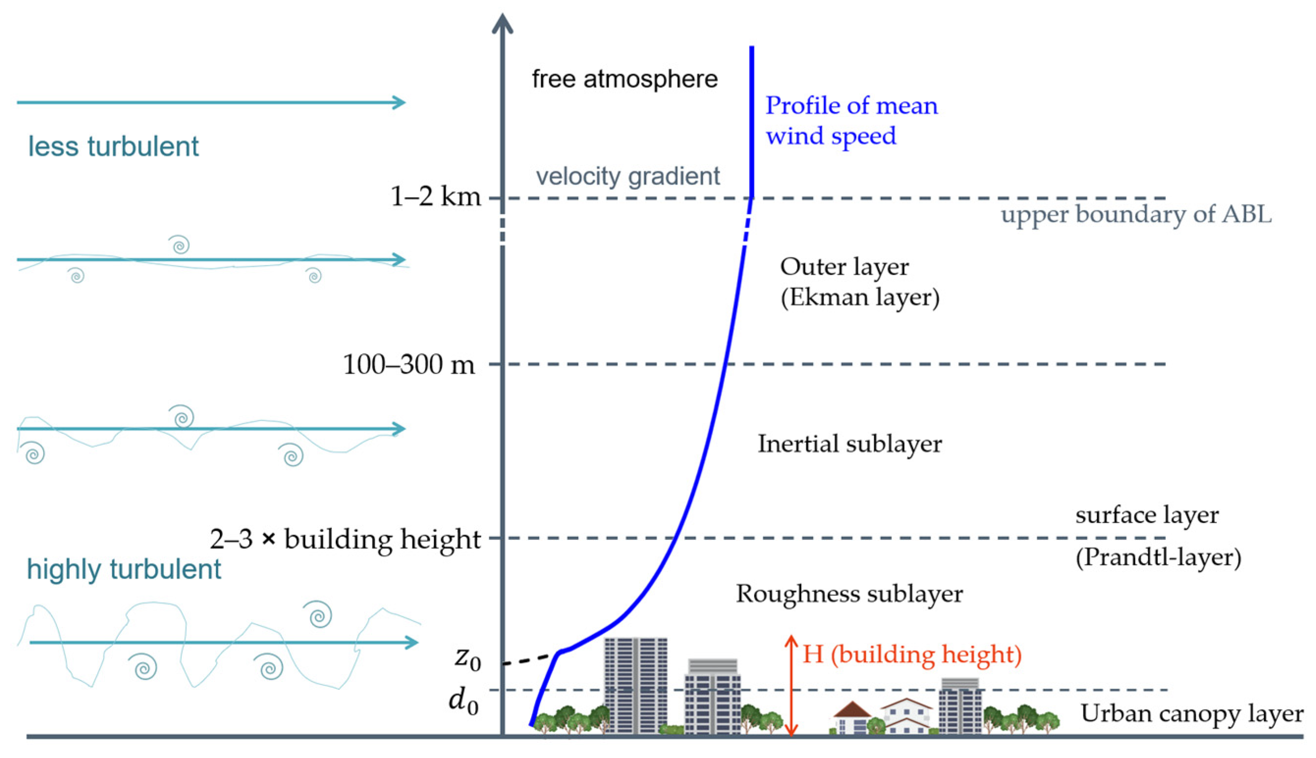
In the atmospheric boundary layer (ABL), two main layers can be distinguished: the surface layer (Prandtl layer) and the outer layer (Ekman layer). In the former, the wind is affected by the presence of the rough surface of the Earth, while in the latter, the wind is influenced by the pressure force (static pressure field) and the Coriolis force due to the Earth’s rotation. In the surface layer there are three sub-layers; in the layer closest to the ground (interfacial sub-layer), depending on the size and density of the roughness, there is no predominant wind direction and the total net flow is zero; thus, the depth of this layer is called zero-plane displacement. The next sublayer is known as the rough sublayer (RS), which is a transition layer between wind’s viscous and inertial sublayers; in the lower part of the RS, the viscous effects predominate followed by a transition zone. As shown in Figure 1, in this rough sublayer, there is an important characteristic height, where the flow velocity is zero, known as the aerodynamic roughness length ; it is related to the average size of the eddies that generate the surface roughness and can be on the order of 10% of the average height of the roughness. The last sublayer is the inertial sublayer (IS), where the inertial effects are more important than the viscous effects.
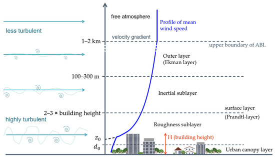
Figure 1.
Atmospheric neutral boundary layer structure.
In a neutral boundary layer, the mechanism of turbulence generation is only mechanical and is associated with shear wind and surface stresses. Then, the similarity theory, which is a type of closure of the zero-order turbulence equations, can be used to estimate values of the mean wind velocity (also temperature, humidity, scalar quantities, etc.) as a function of height, which is:
where is the Von Karman constant (~0.4), is the friction velocity and represents the effect of wind shear stress on the ground. Parameters and are surface properties, determined by the roughness geometry and are independent of wind velocity and wind stability.
The aerodynamic length can be interpreted as the size of a characteristic eddy that is generated as a result of air friction with the ground surface [23]; therefore, it is a function of the size of the surface roughness. If the distribution of roughness elements is very dense, the flow rises above the top of the rough elements and the roughness can be said to form a new rough surface. Mathematically, this change in level is considered by introducing in Equation (1) the displacement .
In the RS, the flow is strongly influenced by the ground surface and is therefore spatially inhomogeneous and inherently three-dimensional. The depth of the RS depends on the shape, size, and distribution or density of the rough elements; therefore, different depths of the RS are to be expected for different terrain types, although it is estimated to be two to five times the height of the rough elements [24].
Finally, as observed in Figure 1, there is a height at which the wind is no longer influenced by the Earth’s surface. This height is referred to as the upper boundary or the boundary layer height, denoted by .
2.2. Flow over a Terrain Change
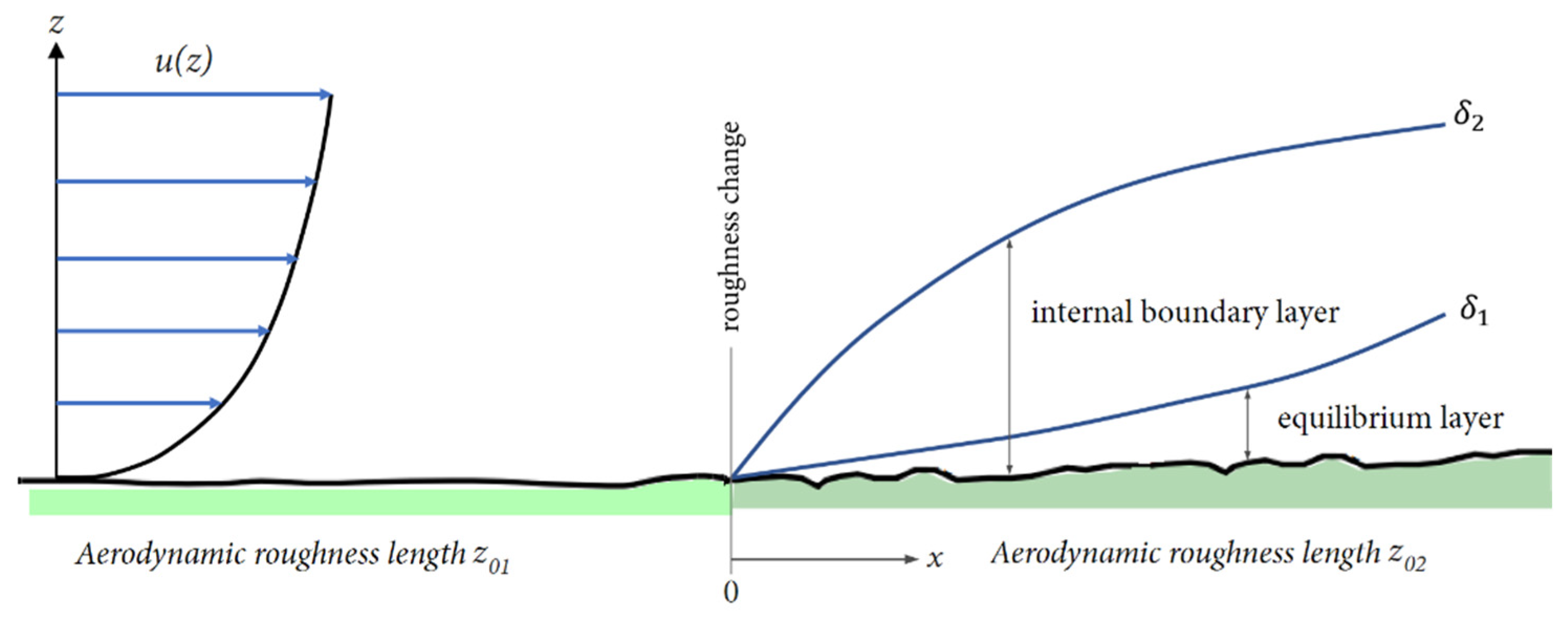
When the wind flows over a terrain with homogeneous roughness, the wind profile is determined by Equation (1), assuming that the boundary layer height is constant. If the ground surface experiences a roughness change, the wind profile tries to adjust to the new terrain: the air moves from terrain with aerodynamic length to another type of terrain with aerodynamic length , which generates the formation of an internal layer , as shown in Figure 2. The wind above height , after the roughness change, depends only on the previous roughness . After the roughness change and below height , the wind speed depends only on the new roughness [25]. The region between and is a transition zone that depends on both roughnesses. The region between the ground and height is called the inner boundary layer and the lower part of this layer (up to height ) is called the equilibrium layer [23,26,27]. It is to be expected that as the wind travel distance increases on the new ground surface, the height of the inner layer will increase until it becomes constant. One particular challenge is defining the height of the inner layer; Cheng and Castro (2002) [24] suggest taking this height as the one where the velocity reaches 99% of the free stream velocity. Several authors have proposed formulations to predict the height of the inner boundary layer, (hereinafter simply referred to as ), in a neutrally stratified flow. Savelyev and Taylor (2005) [28] reviewed several formulations for the evaluation of the inner layer height with the fetch; the same authors [29], based on the derivation of Panofsky and Dutton (1984) [30], proposed an equation for the interface between the incoming flow and the disturbed region (the inner boundary layer) on the grounds that the near-surface air experiences the impact of the roughness change and then propagates upward; they assume that the vertical velocity of propagation is proportional to the variance of the vertical turbulent velocity component, , at the interface , i.e.,
where is a constant. For a steady-state flow, expanding produces , and assuming that is equal to the mean wind velocity and that , Equation (2) is reformulated as
where is another constant, is the mean wind velocity at the interface height and for steady-state flows, and is a function only of the downwind distance .

Figure 2.
Two-dimensional internal boundary layer developing within a constant flux surface layer after a change in surface conditions [28].
Furthermore, considering that the velocity at height , is given by the upwind logarithmic profile
where the subscripts and imply upwind (before roughness change) and downwind values, respectively. Substituting Equation (4) and ( and ) in Equation (3) and integrating, we obtain the model of the form
with as function of . Based on fitting processes for experimental data, we have that
Finally, Savelyev and Taylor (2001) [29] propose the following formula for the internal boundary layer height, , as a function of the fetch, , and roughness change
On the other hand, the equilibrium layer height is usually taken as 10% of the internal layer height and is considered a constant stress layer in equilibrium with the new surface. The growth and adaptation of the flow to the new surface require large distances [26]. If the fetch is not sufficient, the equilibrium layer cannot extend above the rough layer and complicates its identification due to the spatial inhomogeneity of the flow caused by the roughness. To define the logarithmic law parameters (Equation (1)), a constant stress equilibrium layer is required; so, to obtain these parameters for a surface without an equilibrium layer, morphometric methods or surface analysis can be used [31,32].
3. Morphometric Analysis
To describe, model, and forecast the wind behavior in the ABL, it is necessary to derive the aerodynamic characteristics and of the surface, whose effect on the wind depends on the size of the roughness and its distribution or density. Two approaches can be used: morphometric and micrometeorological. The latter uses anemometric field measurements of the wind to determine the aerodynamic parameters of the logarithmic wind profile; the former uses algorithms to relate aerodynamic parameters to the shape and density of the roughness. Morphometric methods have the advantage that parameters can be determined without the need for tall towers and instrumentation at the sites and can also be applied to determine the roughness and its density to generate the required wind profiles when modeling of the atmospheric boundary layer in wind tunnels is required.
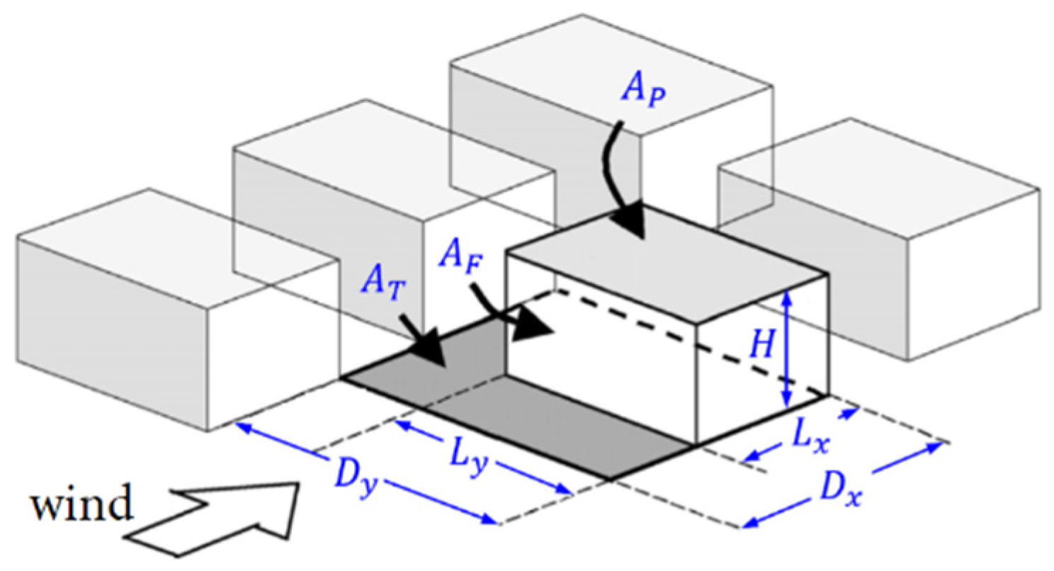
The morphometric methods (according to Figure 3) are divided into three approaches [32]:
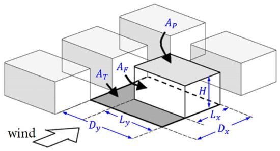
Figure 3.
Dimensions used in morphometric analysis.
- Based on roughness height: ;
- Based on the ratio of the plan area of the obstacles to the lot area: ;
- Based on the ratio of the frontal area of the obstacles to the lot area: .
where and correspond to the plan area and the frontal area of the obstacle, respectively. represents the total lot area. , , and denote the dimensions of the sides and the height of the obstacle. Finally, and are the dimensions of the sides of the total area.
In the simplest method (rule of thumb), and are determined as a fraction of the average height of the roughness elements,
where is the element’s height.
Kutzbach [33], based on field measurements where he placed regularly spaced boxes at different densities on the surface of a frozen lake, proposed:
Lettau [34], based on Kutzbach’s research, proposes Equation (12) to estimate the roughness length for uniformly distributed obstacles.
Counihan [14], from wind tunnel tests and cubic element arrays, determined the expression
where is the fetch and is the plan area of the obstacles. When the fetch is very long, , and the expression reduces to
valid only in the interval .
Theurer [35], using data from city measurements and wind tunnel experiments, found the following expressions (valid for and ) to approximate and .
Kastner-Klein and Rotach [36], from wind tunnel tests, obtain the expression
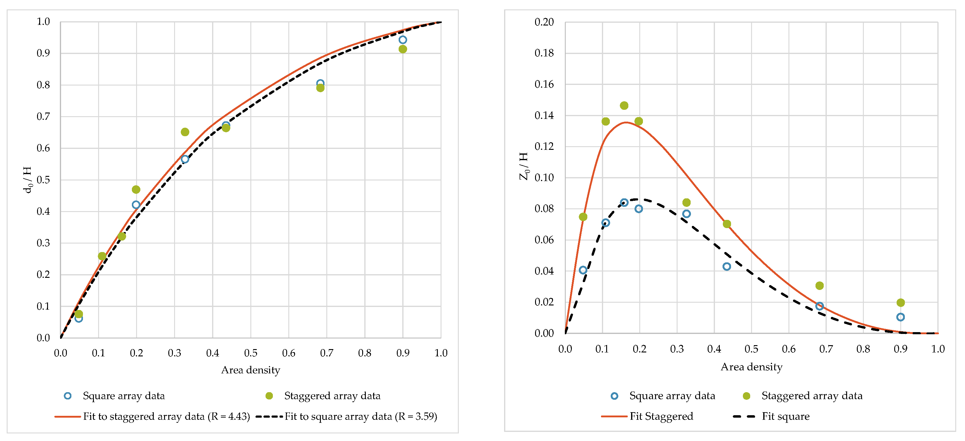
Most of these estimators are limited to rough surfaces with , which is a problem in many practical applications, especially in urban sites where exceeds 20%. Macdonald et al. [32] propose an expression from fundamental principles and basic assumptions, which allows estimating and for densities greater than 30%. They calibrated their formulation with results from wind tunnel tests of different cube arrangements (square and staggered) obtaining:
where is an empirical coefficient, is the drag coefficient of the obstacle (~1.2), is the Von Karman constant, and is a correction factor for the drag coefficient (it considers several variables such as the shape of the velocity profile, the incident turbulence intensity, the scale length of the turbulence, wind incidence angle, and the rounded corners of the cubes). Coefficients and must be established a priori, for example, based on experimental data, and for staggered cube arrays. Figure 4 shows plots of Equations (18) and (19).
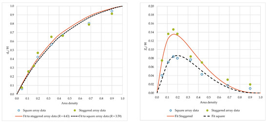
Figure 4.
Plots of and obtained by Macdonald et al. [32].
4. Experimental Study in Wind Tunnel
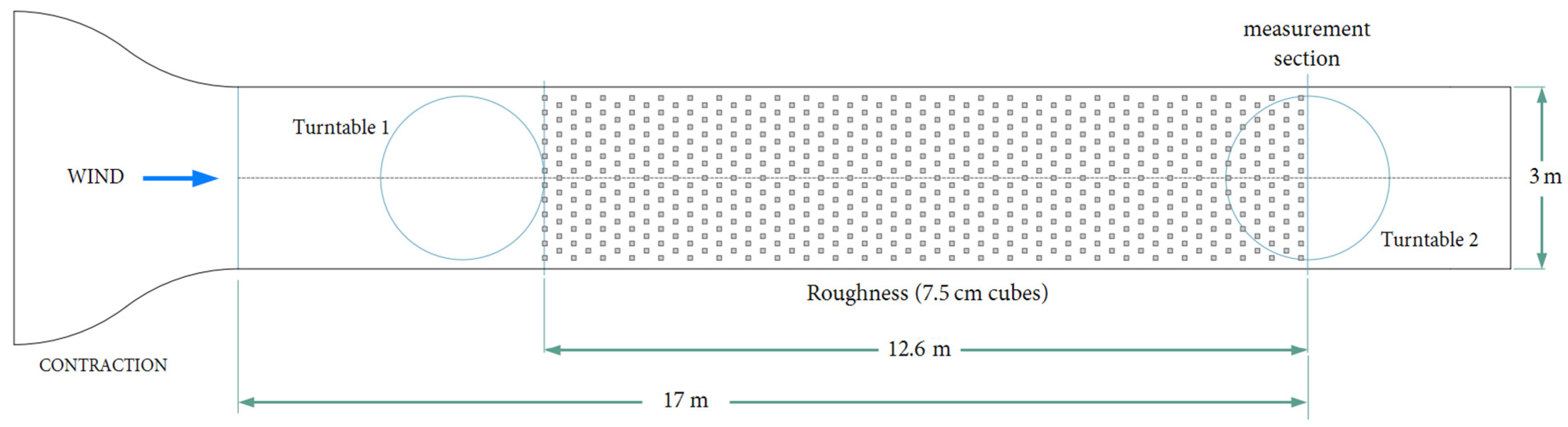
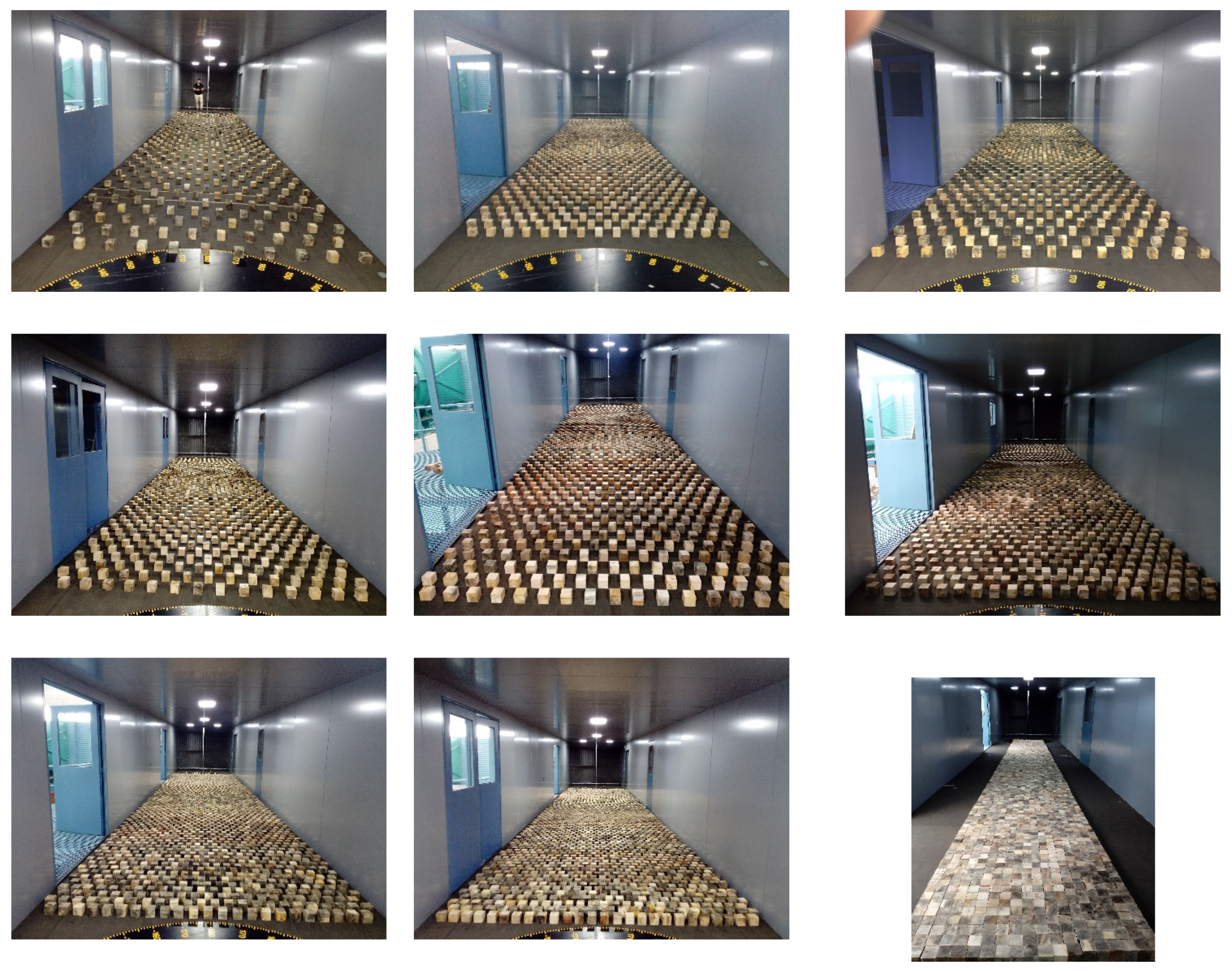
To determine the aerodynamic characteristics ( and ) of a rough surface by means of morphometric analysis, experiments were carried out in a wind tunnel whose test section dimensions are 3 m wide by 2 m high and 17 m long. The rough surface was simulated using cubes of the same dimensions and different densities. Approximately 3100 wood cubes of ~7.5 cm side were utilized. These cubes were arranged in a staggered pattern, creating a flow travel distance (fetch) of 12.6 m. The density cases considered in this study are 0% (no cubes), 2%, 5%, 8%, 10%, 12%, 15%, 20%, 30%, 40%, 50%, and 100% plan area density (e.g., Figure 5 shows a plan view of the cube distribution in the wind tunnel test section for the 10% density case).
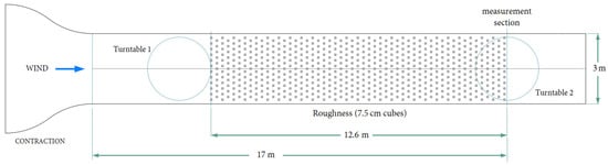
Figure 5.
Plan view of wind tunnel test section with rough elements in a 12.6 m fetch.
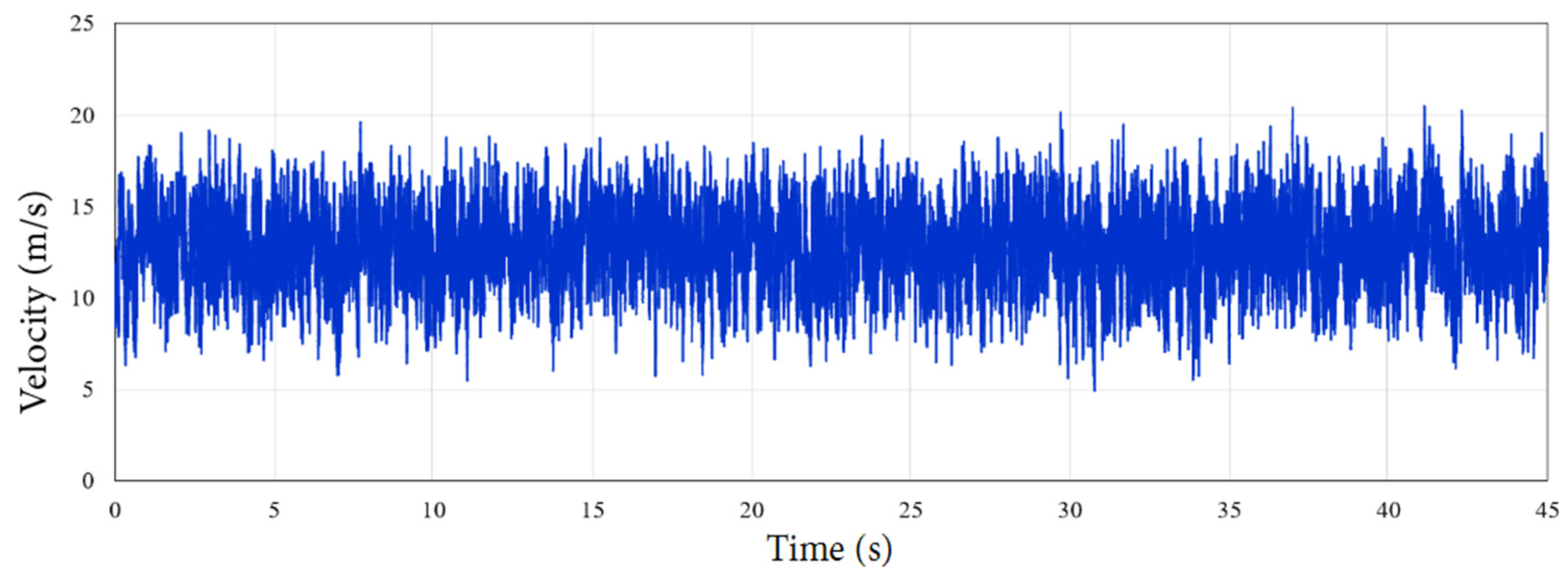
All experimental cases were studied with a mean wind velocity of ~18 m/s (measured at the center of turntable 2 and at a height of 1 m, which corresponds to half the height of the cross-section of the test section of the tunnel under empty tunnel conditions), and this velocity could represent an upper limit for the various tests required in wind tunnel studies. The wind speed profiles were measured with a hot wire anemometer placed at the center of turntable 2 (see Figure 5), with a sampling frequency of 2 kHz and a total time of 60 s. Figure 6 shows a typical record and Figure 7 shows the arrangements of cubes in the wind tunnel tests for all cases considered.

Figure 6.
Typical wind velocity record (record measured at a height of 3H for the case of = 50%).
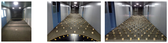

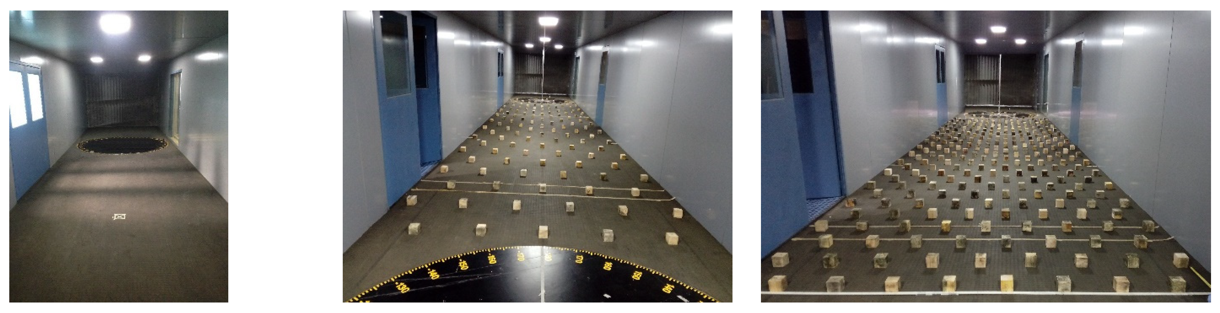
Figure 7.
Arrangement of cubes in the wind tunnel for the different cases of roughness density considered: 0%, 2%, 5%, 8%, 10%, 12%, 15%, 20%, 30%, 40%, 50%, and 100%. In all cases, cubes of the same dimensions were used (~7.5 cm side).
4.1. Fitting of Aerodynamic Surface Characteristics
To estimate the displacement height , Equation (18), proposed by Macdonald et al. [32], with (for staggered cube arrays) was used, since this equation is applicable to the whole range of densities, and according to Grimmond and Oke [31], the values predicted by this equation are reasonable. The friction velocity was estimated by linear regression (Equation (20)) with the profile data measured in the tunnel and represented with a plot of velocity versus log10 of the height. The roughness length, , was estimated using the Generalized Reduced Gradient (GRG) nonlinear optimization method [37], implemented in the solver of Microsoft Excel software. The GRG method is among the most popular approaches for solving nonlinear optimization problems, requiring only that the objective function be differentiable. The main idea of this method is to solve nonlinear problems dealing with active inequalities. Variables are divided into two groups: basic (dependent) variables and nonbasic (independent) variables. The reduced gradient is then calculated to identify the minimum in the search direction. This process is repeated until the convergence is obtained. The estimates of and have been corroborated with the modified Clauser chart method.
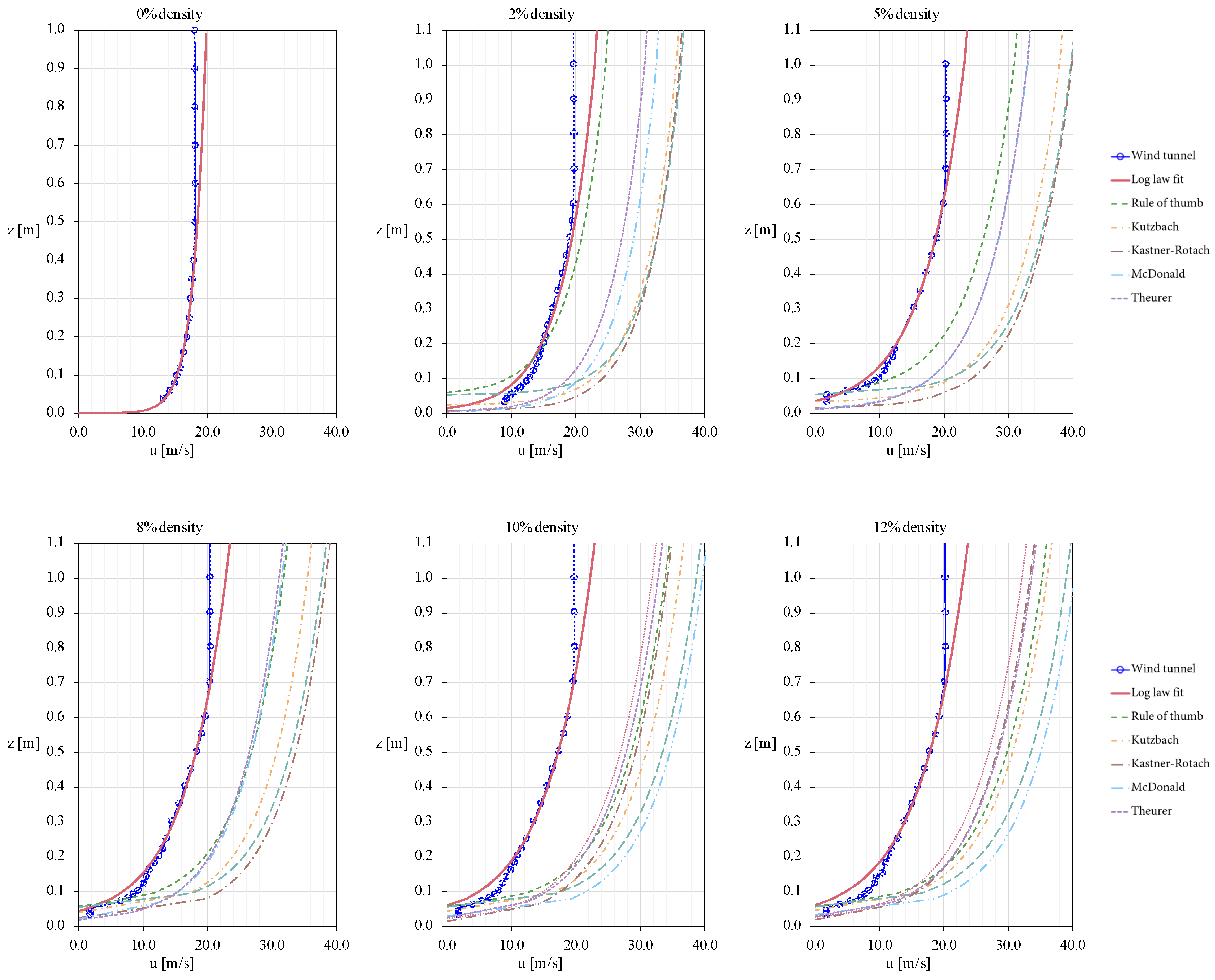
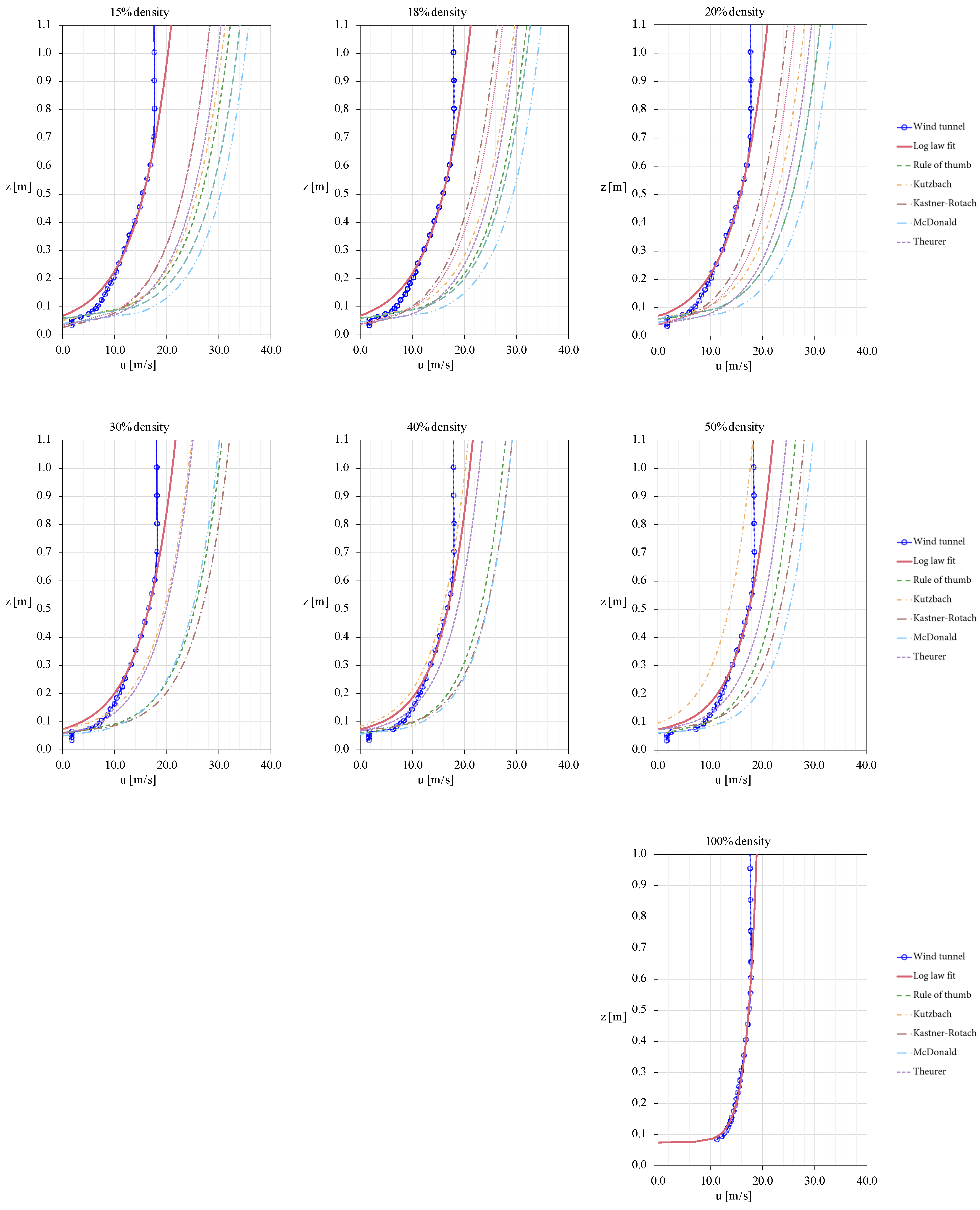
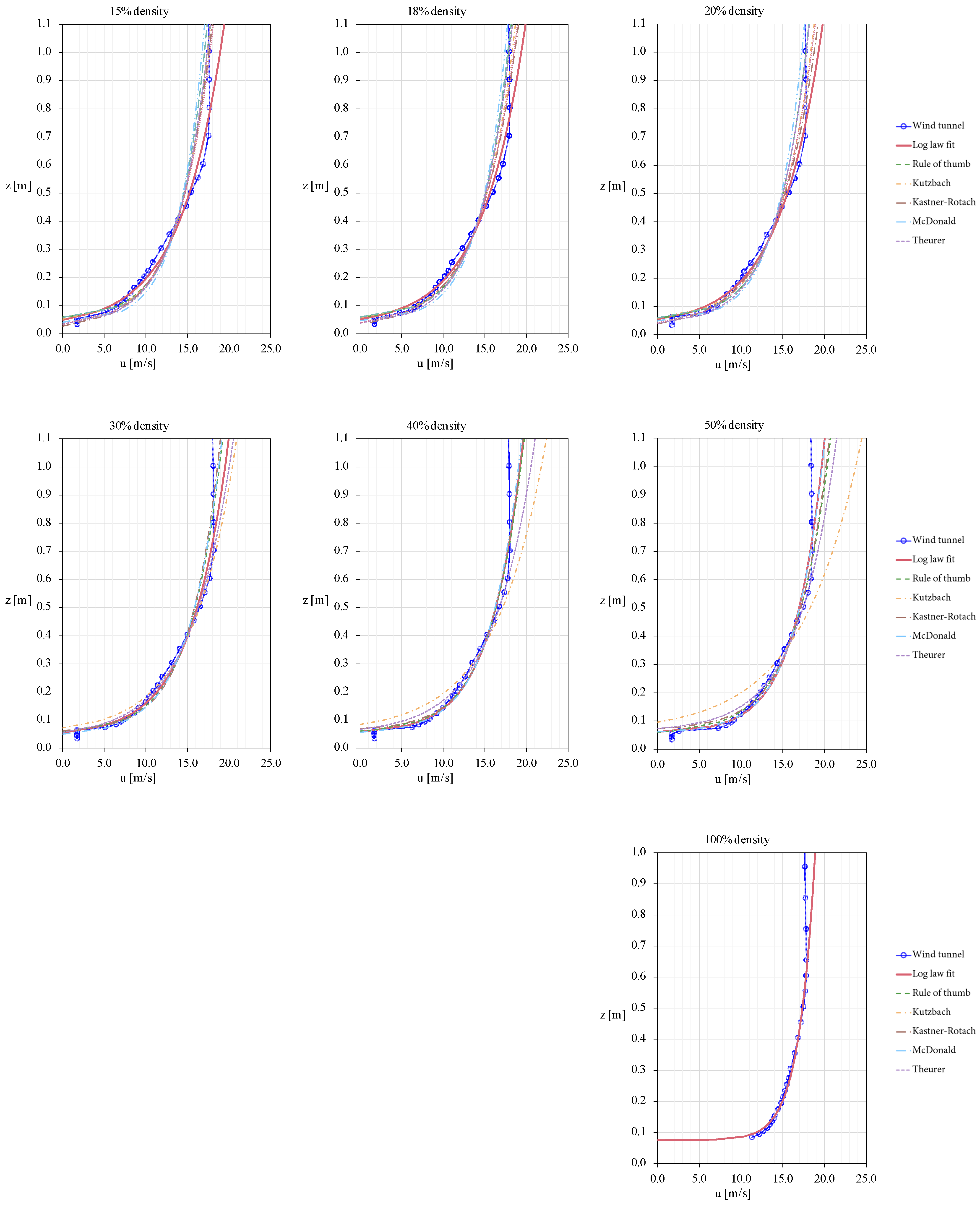
Table 1 shows the estimated values for , , and for both those fitted to the experimental data and the formulations proposed by several authors mentioned in Section 2. The same estimated with the fit to the experimental data was used for all formulations, except for formulations that do not include an estimate of , where we used the one estimated by the rule of thumb (). Figure 8 shows the measured wind speed profiles (blue circles), the profile fitted to the logarithmic law (red line), and the profiles obtained by several authors. It can be seen that Equation (1) (with the estimated values for , and ) and the experimental data have a similar trend in shape and magnitude up to the height of the boundary layer (~60 cm). Differences in near-surface wind speeds (rough sublayer) can also be appreciated. This behavior might be related to the fact that, strictly speaking, the logarithmic law (log law) is only applicable in the inertial sublayer (IS), which starts well above the height of the rough elements (two to three times the height of the roughness), since the rough sublayer (RS) is a transition layer between viscous and inertial effects and in the IS the turbulent flows are approximately constant. This can be seen in the data fits shown in Figure 8, where the log law fits the data from a height of 0.22 m (approximately three times the height of the cubes) and up to a height where the velocity is practically constant (approximately 0.99 umax). Figure 8 also shows the profiles obtained by several authors, and it is observed that they are similar to the experimental data in shape but different in magnitude; therefore, for comparison purposes, it is necessary to normalize the profiles with the friction velocity . Since in the references of some authors the value of is unreported, an independent estimation is made for each formulation (as will be shown hereafter in the second estimation).

Table 1.
Experimental fitting of the aerodynamic parameters and for formulations by various authors; see Section 2 [first estimate].
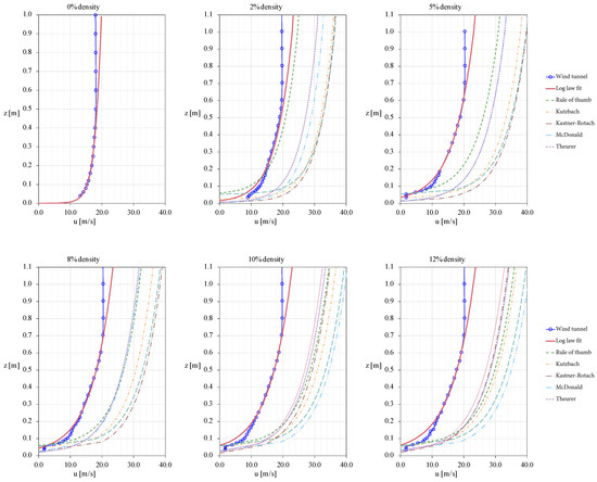
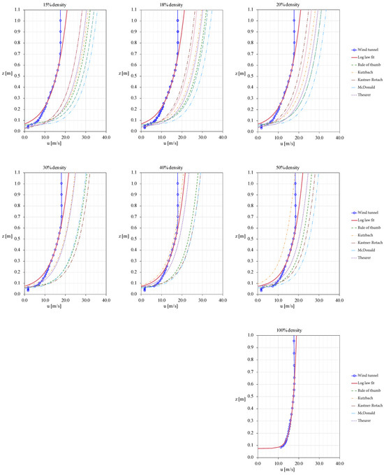
Figure 8.
Measured profiles of mean wind velocity, logarithmic law fit, and profiles of the formulations presented in Section 2 (first estimation).
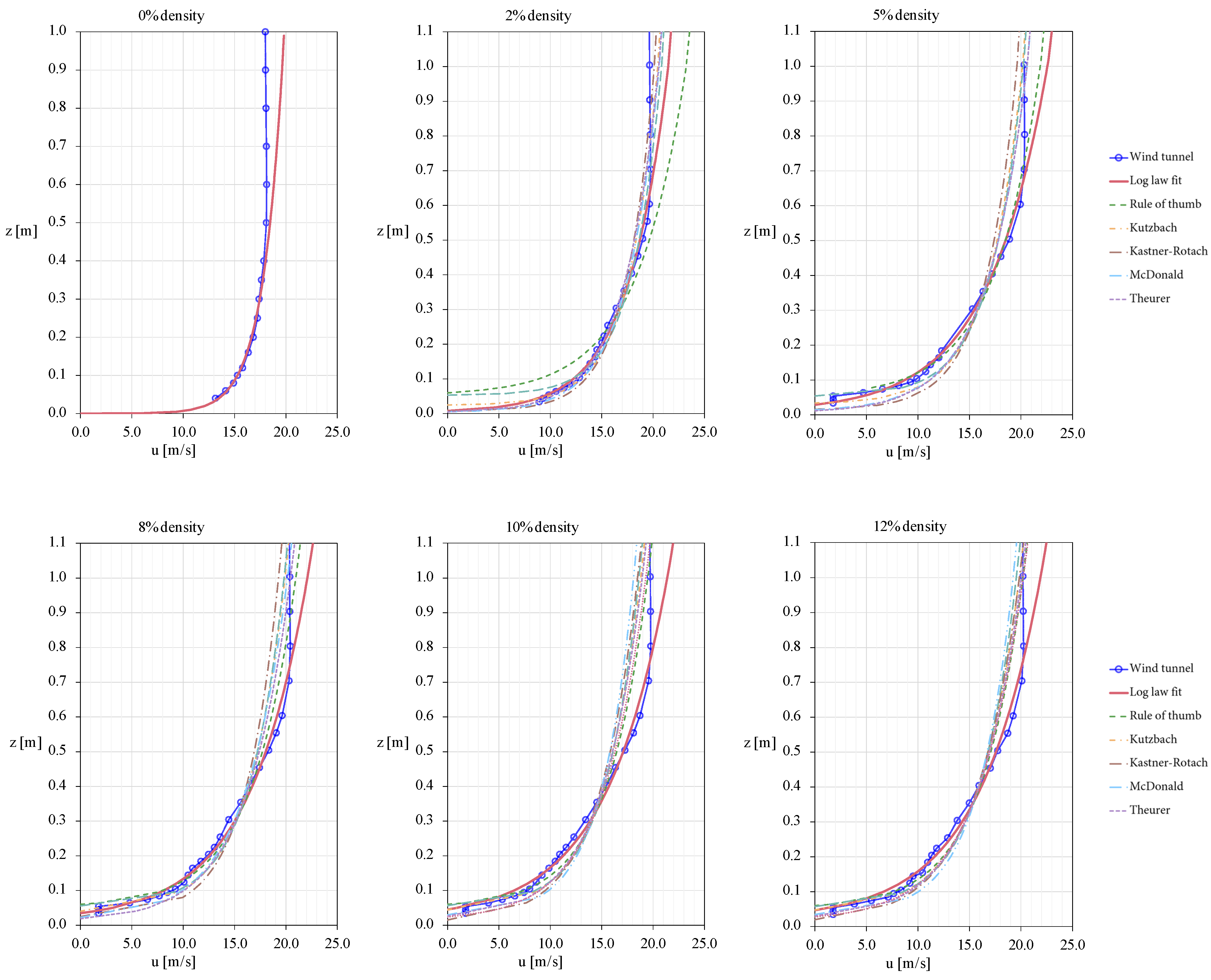
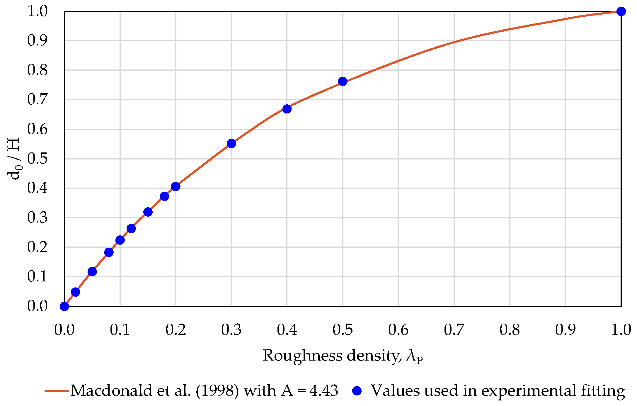
Because the objective of this study is to perform parameterizations that allow estimating the mean wind speed profiles even in the rough sublayer, a second fit to the experimental data was performed. For this second trial, both parameters, and , were estimated by the generalized reduced gradient nonlinear optimization method, both for the experimentally measured data and the formulations proposed by other authors. To determine the wind velocity profiles using the morphometric formulations by different authors presented in Chapter 3, and given that the friction velocity estimated by these authors in their experiments is unknown, the value of was calculated for each formulation through an adjustment using the GRG method, based on the experimentally obtained data. Because the rough sublayer is involved in this estimate, should be interpreted as a scaling velocity for the mean wind profile, rather than as an estimate of a real friction velocity. Table 2 presents the new estimated values for , , and and Figure 9 shows the wind speed profiles obtained with this second estimation. The experimental values of the parameters , , and are summarized in Table 3, where the boundary layer depth , estimated as 0.99 of the maximum velocity, is also presented. With this second trial, a better fit to the experimental data is obtained, especially in the rough sublayer, so the values of and obtained are normalized with the cube height () for each cube density case (see Table 4). Figure 10 shows the variation in the parameterization as a function of the roughness density, and this relation was used in the fitting to the log law (in principle it was established that it should coincide with the curve proposed by Macdonald et al. [32]). It is observed that for a density of 100%, , since there is no separation between the roughnesses and a new planar surface without obstructions is generated.
Table 2.
Experimental fitting of the aerodynamic parameters and for formulations by various authors [second estimate].
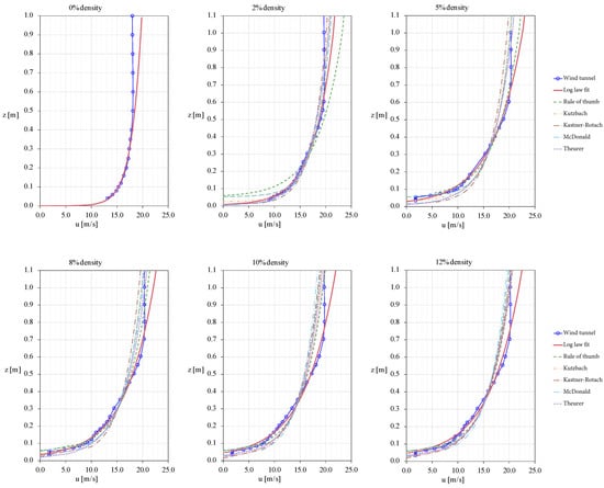
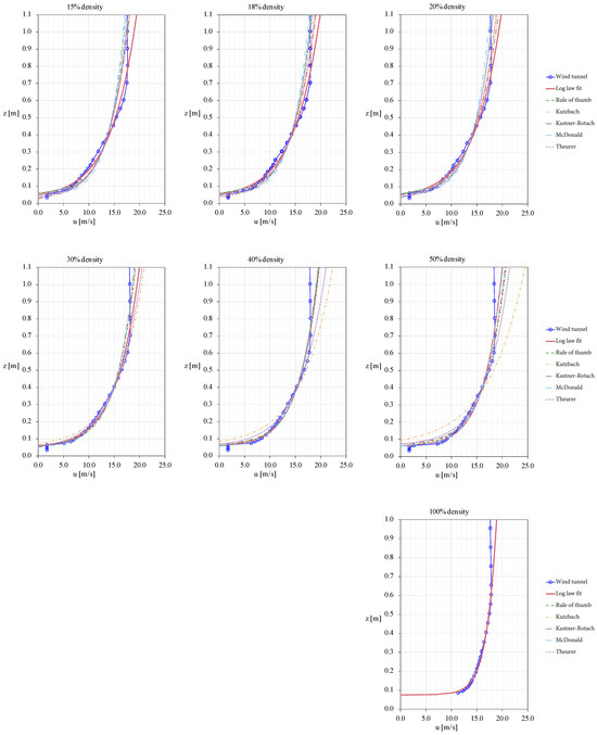
Figure 9.
Measured profiles of mean wind velocity, logarithmic law fit, and profiles of the formulations presented in Section 2 (second estimation).
Table 3.
Summary of surface aerodynamic parameters.
Table 4.
Parameterization of , , and .

Figure 10.
Plot of the variation and values used in experimental fitting [32].
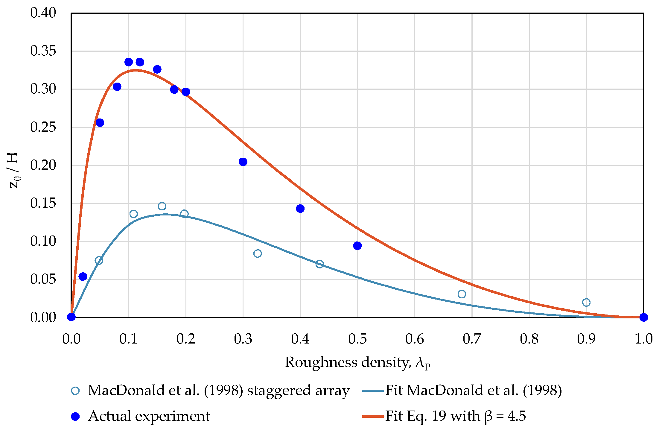
Regarding , the variation in as a function of roughness density and its comparison with the experimental data obtained by Macdonald et al. [32] is presented in Figure 11. It can be seen that there are differences between the results which, according to Macdonald et al. [32], may be associated to several variables, such as fetch length, cube material, cube shape, velocity profile shape, incident turbulence intensity, turbulence scale length, wind angle of incidence, and rounded corners of the cubes, in addition to the fact that the adjustment also takes into account the rough sublayer. By fitting Equation (19) to the experimental data of this study, a value of 4.5 for the correction factor was determined, and this curve is also shown in Figure 11.
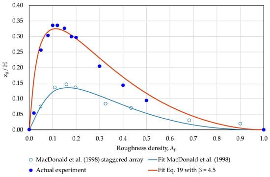
Figure 11.
Plot of the de variation for the current experiment and fit to Equation (19) with , compared with the results of Macdonald et al. [32].
4.2. Boundary Layer Depth
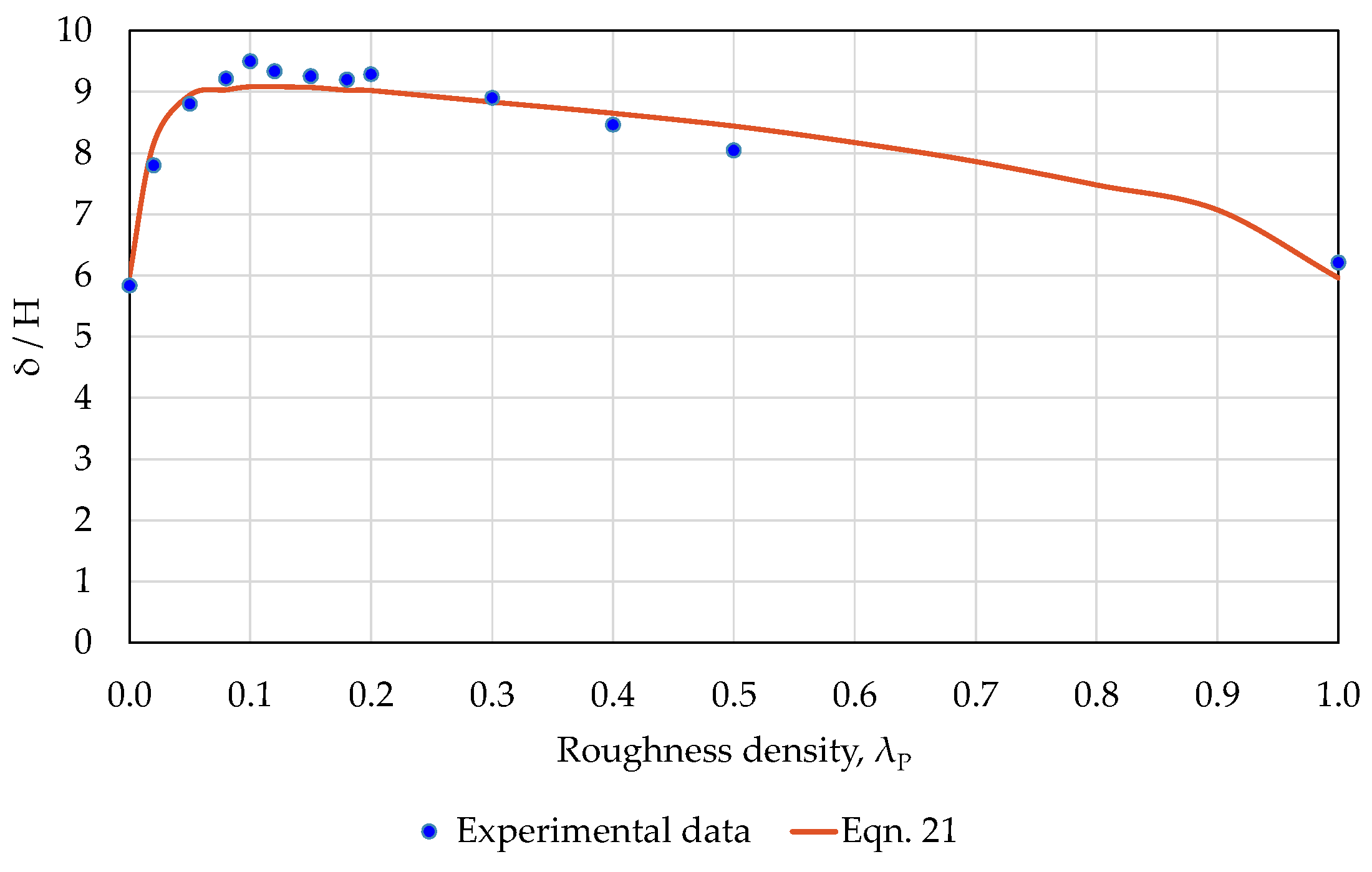
Another variable of interest in this study is the magnitude of the boundary layer height. Based on the formulation proposed by Savelyev and Taylor [28], see Equation (7), and with the experimental data of the boundary layer height shown in Table 3, an equation which relates the boundary layer height to the fetch and the aerodynamic lengths of the surfaces was derived, as follows:
where is the fetch (in this case ).
Table 4 shows the parameterization of the boundary layer depth with the height of the roughness and Figure 12 shows the variation in the boundary layer height (normalized with the height of the cubes) with respect to the roughness density and the fitting curve obtained by Equation (21).

Figure 12.
Plot of the variation for the current experiment (with fetch ).
4.3. Turbulence Intensity
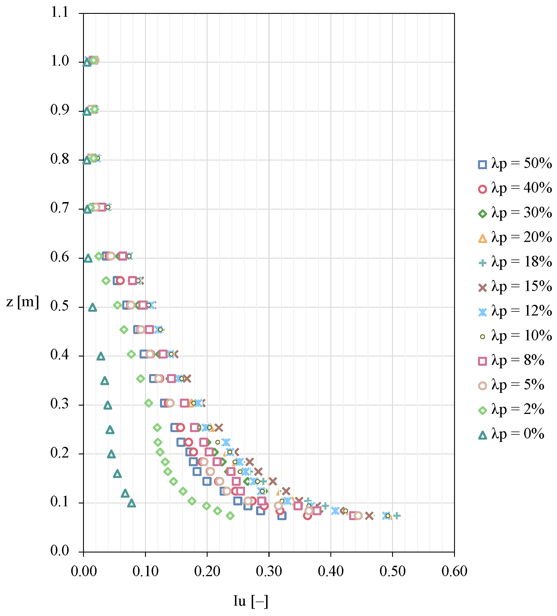
In wind tunnel simulations of the ABL, it is also important to characterize the longitudinal turbulence intensity, , defined as the standard deviation of the wind speed divided by the mean velocity; it was calculated using the experimental data and the results are shown in Figure 13 for each roughness density case. To derive a fitting curve that has the best fit of the turbulence intensity as a function of height and parameter , the following model for the turbulence intensity is proposed:
where and are model fit parameters, whose estimated values are presented in Table 5.
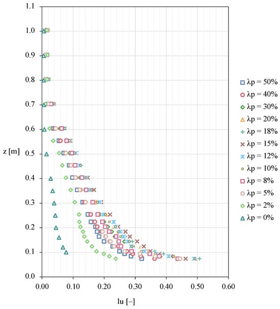
Figure 13.
Experimental turbulence intensities for each roughness density case.
Table 5.
Fitting of parameters and of Equation (22).
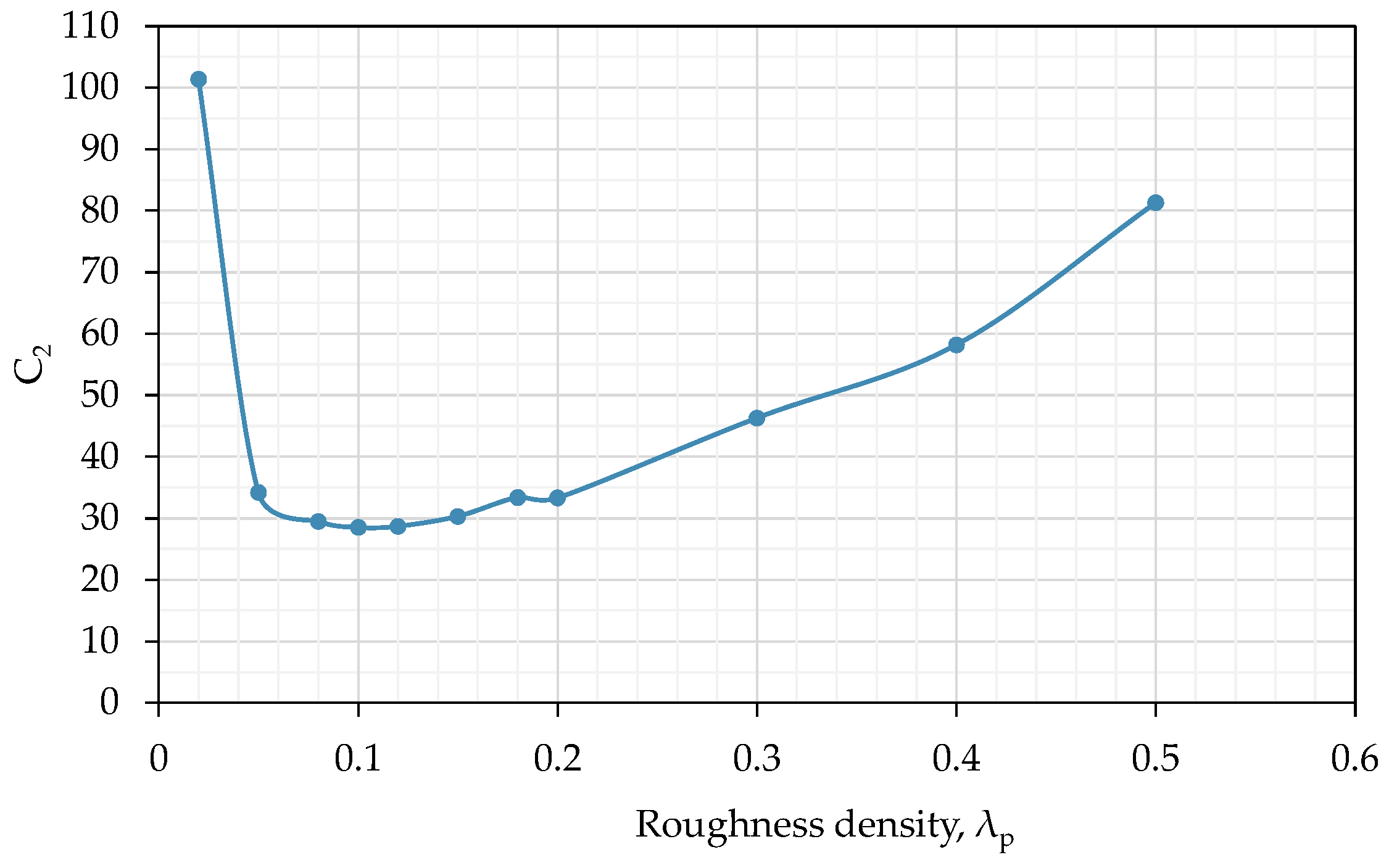
From the data in Table 5, a constant value equal to 0.09 (approximately the average of the cases producing the most turbulence: to ) is proposed for , resulting in:
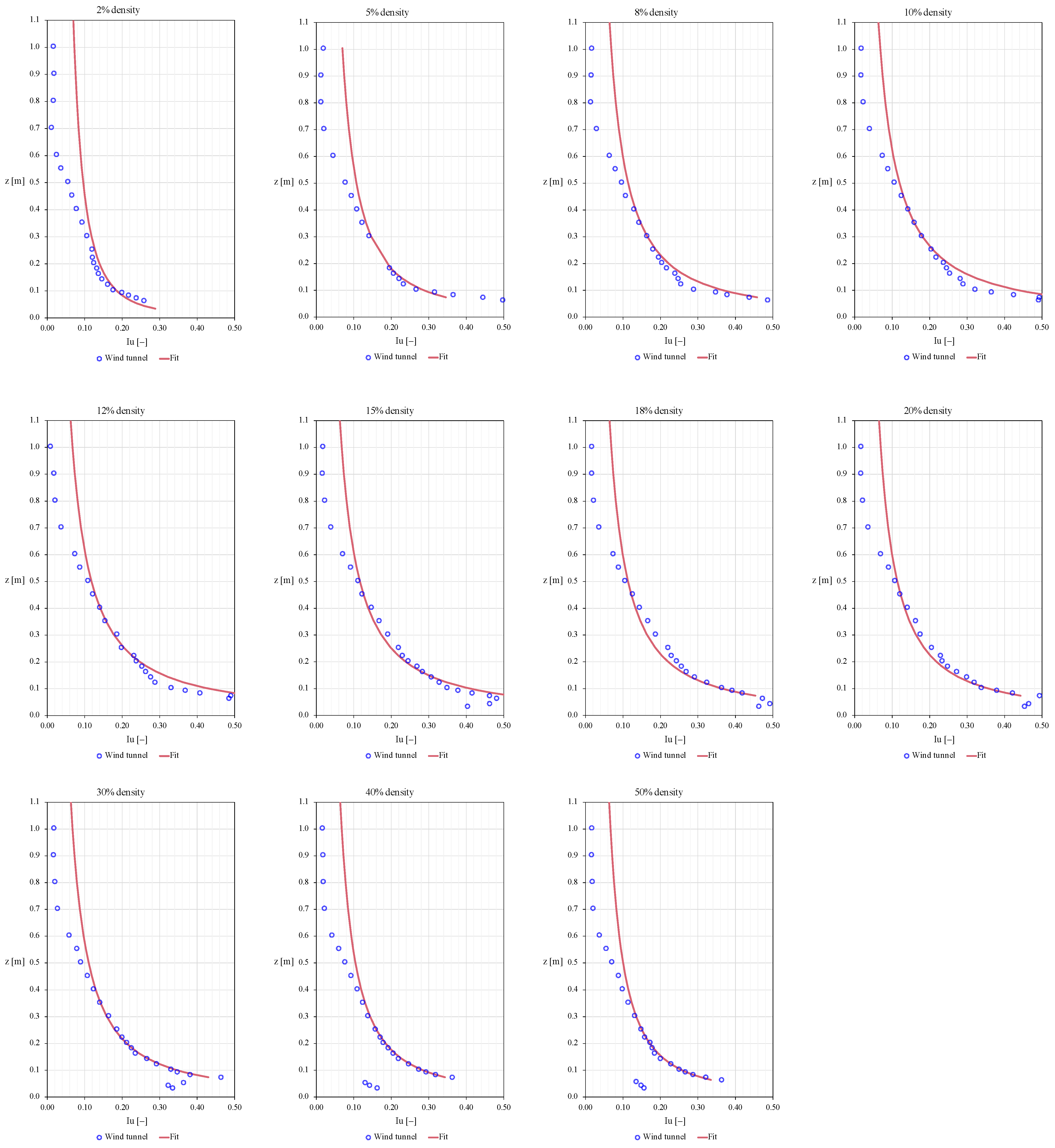
With this value of , another fitting process was conducted. Table 6 shows the new results of , and its variation with respect to the density of roughness elements is presented in Figure 14. Figure 15 shows plots of the experimental turbulence intensity profiles (see Figure 14) for each density case studied, together with the result of applying Equation (23). A good fit of Equation (23) with the experimental data can be seen from the height of the rough elements (7.5 cm) up to the height of the boundary layer (approximately 60 cm).
Table 6.
Estimation of parameter in Equation (23).
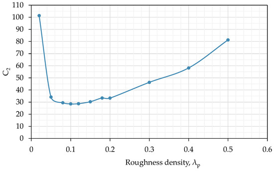
Figure 14.
Curve of the parameter (Equation (23)) depending on area density of roughness elements.
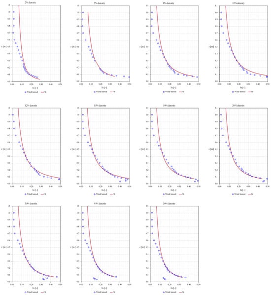
Figure 15.
Experimental turbulence intensities and fit to Equation (23).
Finally, and according to the previous data shown in Figure 14, it is proposed to use the value of in Equation (24) for densities between 5% and 22% (which would probably be the most useful in wind tunnel boundary layer simulation due to the levels of turbulence generated) and a linear interpolation of for densities between 22% and 50%. Thus,
4.4. Spectral Density Function
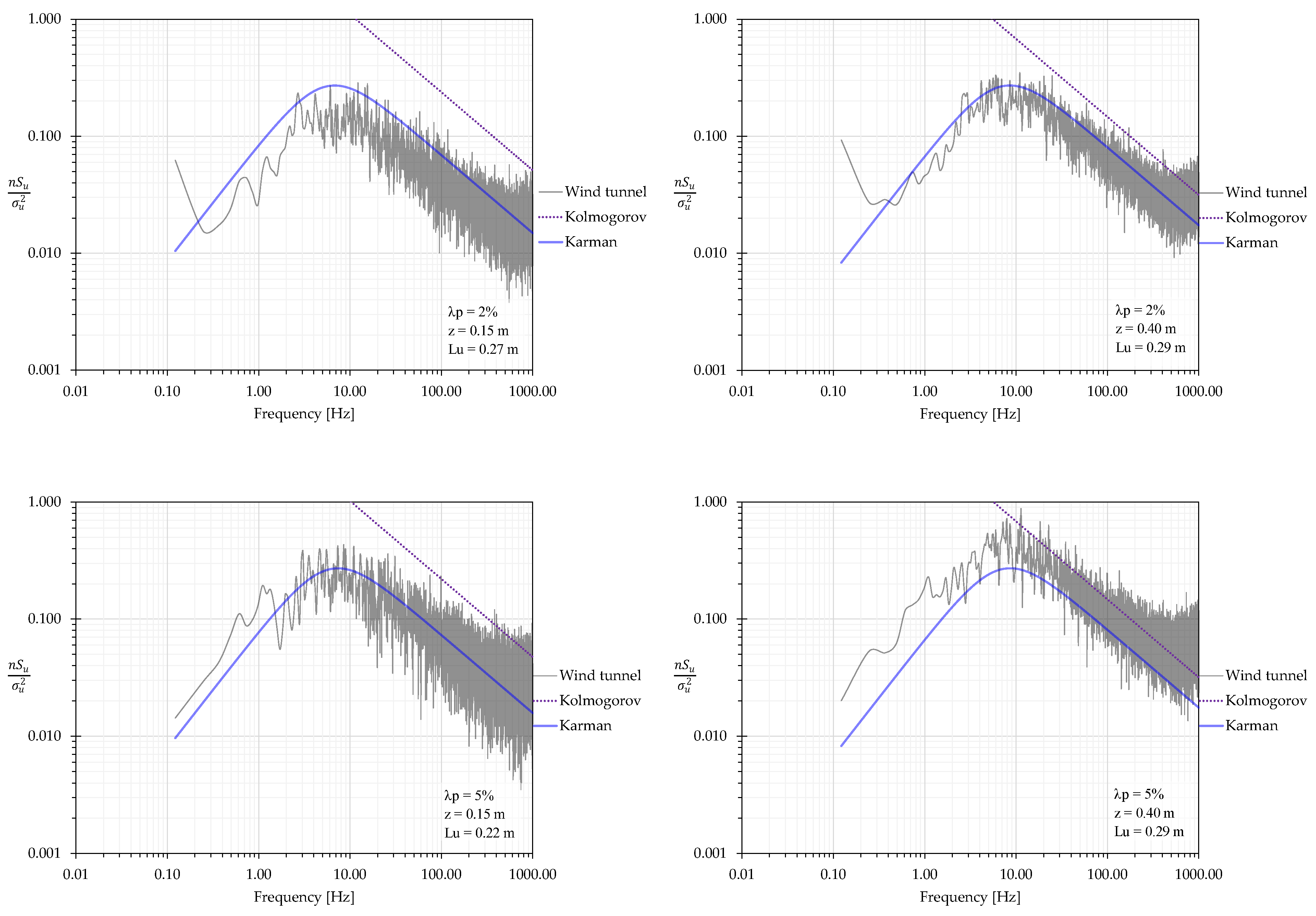
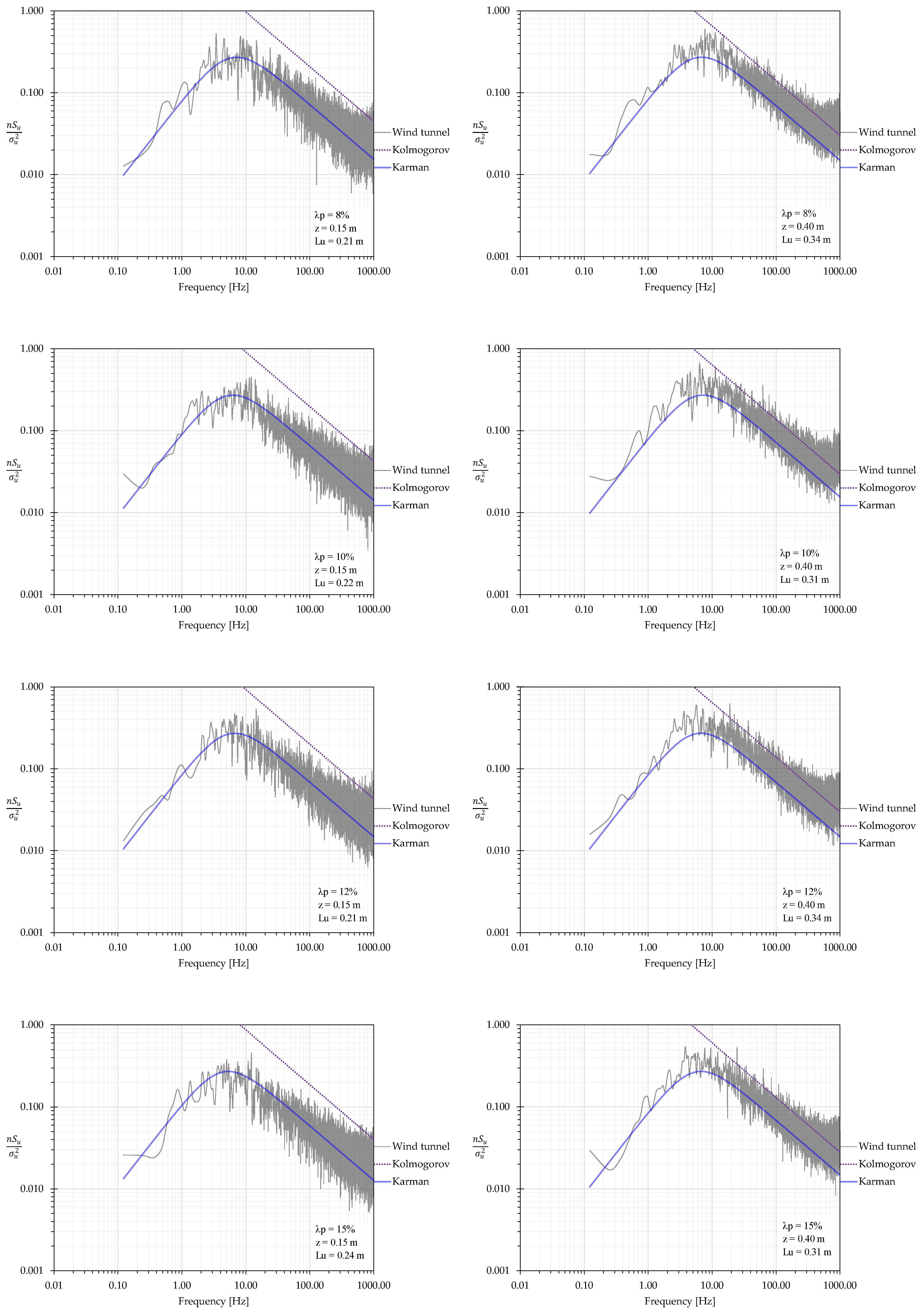
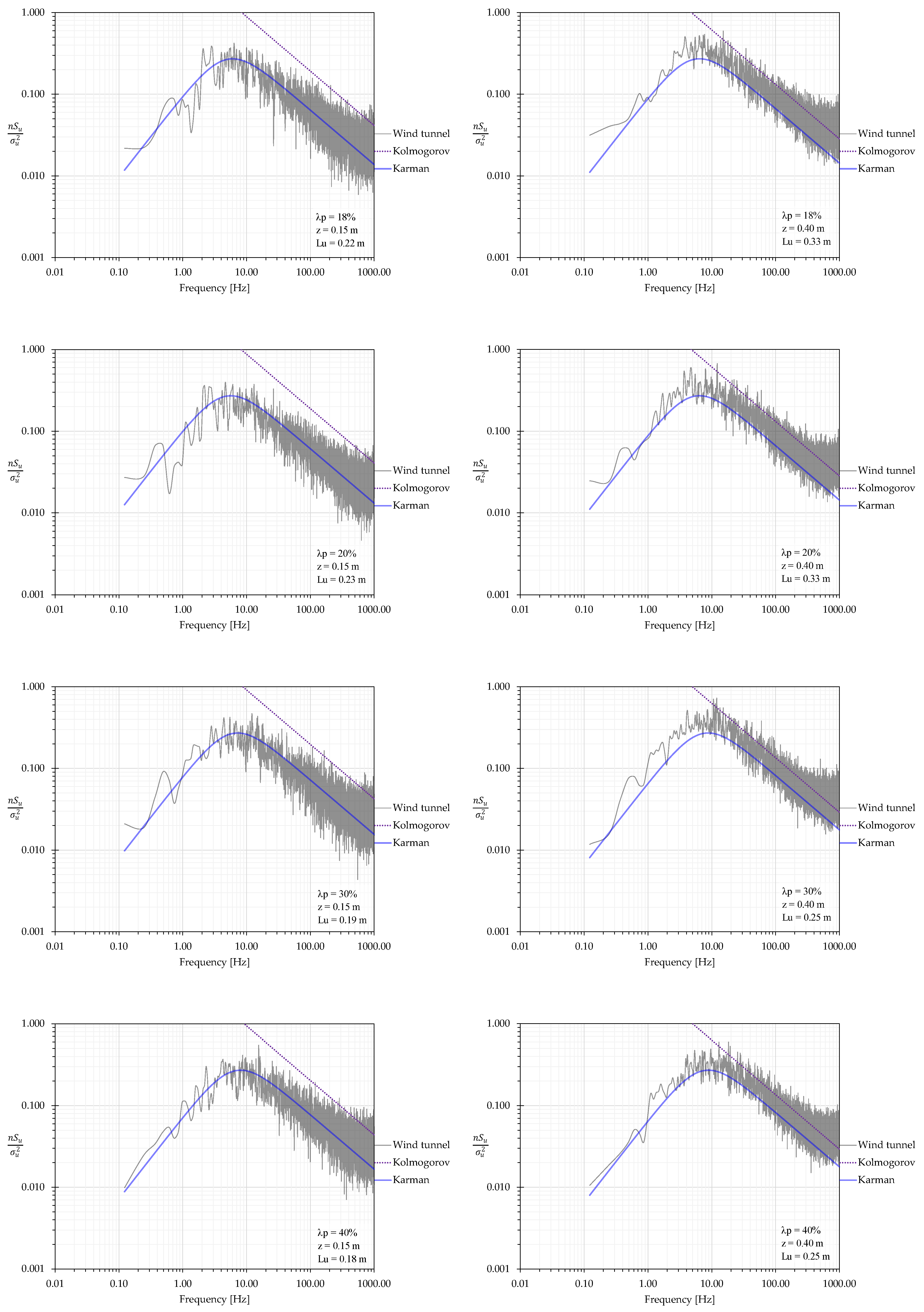
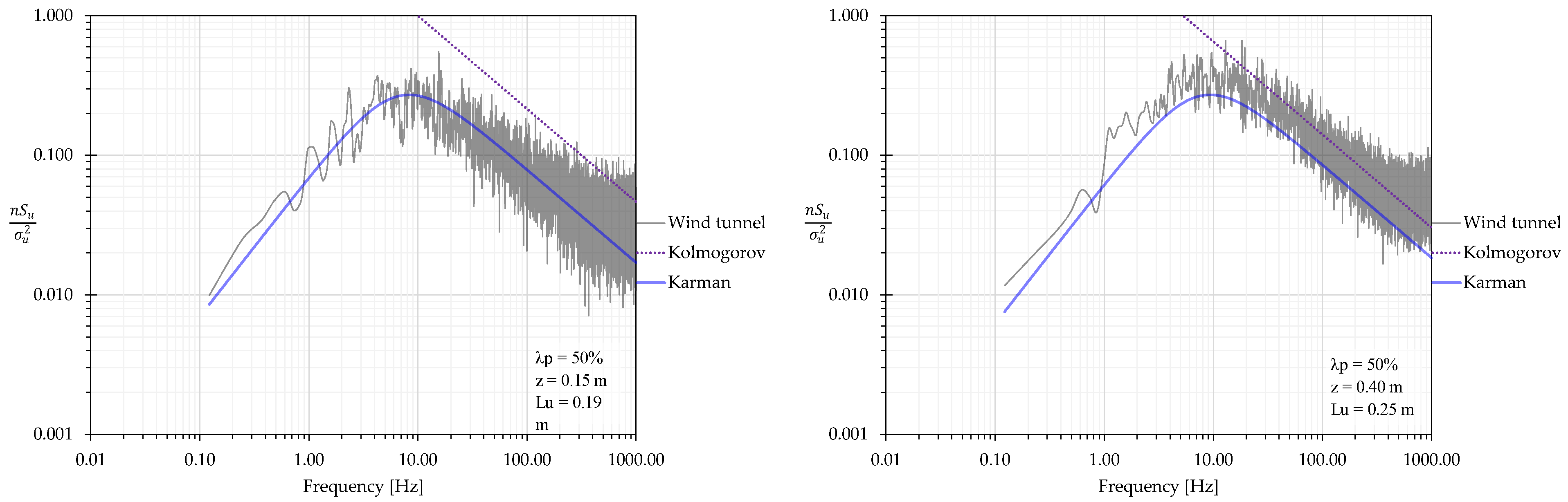
Turbulence spectra are statistical parameters used to compare the characteristics of wind velocity fluctuations between atmospheric conditions and tunnel simulations. Based on experimental measurements and using the Welch method [38], the turbulence spectra or spectral density functions were estimated and are shown in Figure 16. In this study, spectral density functions were calculated at two heights: approximately 15 cm, corresponding to the middle of the rough sublayer, and approximately 40 cm, corresponding to the middle of the inertial sublayer. Figure 16 compares the experimental spectra with Kolmogorov’s 5/3 law and the Von Kármán spectrum (Equation (25)).
where
where represents the frequency, denotes the power spectrum density, is the standard deviation, signifies the mean wind speed, and indicates the turbulence length scale.
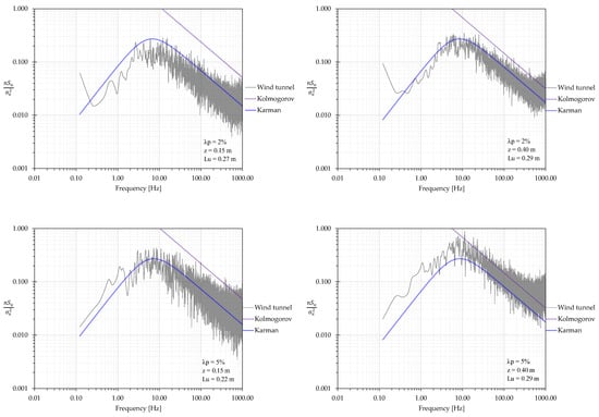
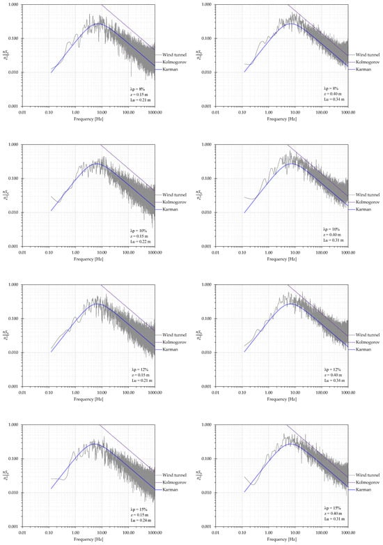
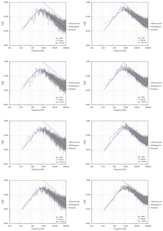
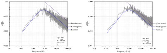
Figure 16.
Spectral density functions measured at heights of 0.15 m, corresponding to half the height of the rough sublayer (left side), and 0.40 m, representing half the height of the inertial sublayer (right side).
In this paper, the integral length scale of velocity is determined by Trush et al. [39]:
where indicates the autocorrelation function (i.e., correlation of a velocity component with itself) and r is the spatial lag.
In general, it can be noted that the experimental spectra obtained show adequate convergence with the theoretical Von Kármán spectrum. A good fit to the experimental data is observed, both in the rough sublayer and the inertial sublayer.
5. Discussion and Conclusions
The main objective of this study is to relate the aerodynamic characteristics of the rough surface, considered in the logarithmic wind law (zero-plane displacement plane and aerodynamic roughness length ), to the geometry and density of the rough elements of a rough surface in order to simulate the neutral atmospheric boundary layer in a wind tunnel.
To achieve this goal, a series of wind tunnel experiments were performed using cubes as rough elements placed in staggered arrangements and using different densities. By means of morphometric methods, it was possible to establish a parameterization of the aerodynamic parameters and of the wind profile as a function of the geometry of the cubes and their density. In general, it can be concluded that the log law can adequately describe the wind velocity profiles measured in the experiments, with slight differences in the rough sub-layer due to the fact that in this zone the surface stresses are not constant.
If required, an adequate description of the wind profile in the inertial sublayer by means of the log law should apply Equation (20) for an adequate estimate of the frictional velocity . Estimates of based on the fits, even in the rough sublayer (second estimate, Table 2), should be interpreted as a scaling velocity for the mean wind profile, rather than an estimate of an actual friction velocity.
Based on the study of Savelyev and Taylor, it was also possible to adjust a formulation for the growth of the boundary layer height as a function of the fetch and the change in the aerodynamic surface length. It is important to mention that Equation (21) was derived for the case where the fetch is 12.6 m. For a better prediction or calibration of Equation (21), it is suggested to perform experiments considering different fetch lengths.
In addition, considering a neutral boundary layer, a formulation was established to estimate the vertical profile of turbulence intensity (Equation (23)) for different roughness densities (cubes). Figure 15 shows that Equation (23) estimates adequately profiles over the entire boundary layer interval with an average height of 65 cm.
Finally, from the convergence of the experimental turbulence spectra with theoretical functions, it can be concluded that statistically there is a good similarity between the flow generated in the laboratory and the atmospheric ones.
Author Contributions
Conceptualization, R.S.-G. and R.G.-M.; methodology, R.S.-G.; software, R.S.-G.; validation, R.S.-G. and R.G.-M.; formal analysis, R.S.-G. and R.G.-M.; investigation, R.S.-G.; resources, R.G.-M.; data curation, R.S.-G.; writing—original draft preparation, R.S.-G.; writing—review and editing, R.S.-G. and R.G.-M.; visualization, R.S.-G.; supervision, R.G.-M. All authors have read and agreed to the published version of the manuscript.
Funding
This research received no external funding.
Institutional Review Board Statement
Not applicable.
Informed Consent Statement
Not applicable.
Data Availability Statement
Dataset available on request from the authors.
Acknowledgments
We gratefully acknowledge funding from the Consejo Nacional de Ciencia y Tecnología, particularly grant 859613, and the Universidad Nacional Autónoma de México. Thanks are expressed to Óscar N. Rosales, L. Martín Arenas, and Marco A. Mendoza for their technical support in the wind tunnel tests. The authors sincerely appreciate the insightful comments provided by the reviewers, which have greatly contributed to enhancing the quality of this work.
Conflicts of Interest
The authors declare no conflicts of interest.
References
- Van der Hoven, I. Power spectrum of horizontal wind speed in the frequency range from 0.0007 to 900 cycles per hour. J. Meteorol. 1957, 14, 160–164. [Google Scholar] [CrossRef]
- Solari, G. Wind Science and Engineering: Origins, Developments, Fundamentals and Advancements; Springer: Basel, Switzerland, 2019. [Google Scholar]
- Davenport, A.G. A Statistical Approach to the Treatment of Wind Loading on Tall Masts and Suspension Bridges. Ph.D. Thesis, University of Bristol, Bristol, UK, 1961. [Google Scholar]
- Hu, W.; Yang, Q.; Peng, L.; Liu, L.; Zhang, P.; Li, S.; Wu, J. Non-stationary modeling and simulation of strong winds. Heliyon 2024, 10, e35195. [Google Scholar] [CrossRef] [PubMed]
- Hangan, H.; Romanic, D.; Jubayer, C. Three-dimensional, non-stationary and non-Gaussian (3D-NS-NG) wind fields and their implications to wind–structure interaction problems. J. Fluids Struct. 2019, 91, 102583. [Google Scholar] [CrossRef]
- Huang, M.; Li, Q.; Xu, H.; Lou, W.; Lin, N. Non-stationary statistical modeling of extreme wind speed series with exposure correction. Wind. Struct. 2018, 26, 129–146. [Google Scholar] [CrossRef]
- Jiang, F.; Zhang, M.; Li, Y.; Zhang, J.; Qin, J.; Wu, L. Field measurement study of wind characteristics in mountain terrain: Focusing on sudden intense winds. J. Wind. Eng. Ind. Aerodyn. 2021, 218, 104781. [Google Scholar] [CrossRef]
- Liu, Y.X.; Hong, H.P. Analyzing, modelling, and simulating nonstationary thunderstorm winds in two horizontal orthogonal directions at a point in space. J. Wind. Eng. Ind. Aerodyn. 2023, 237, 105412. [Google Scholar] [CrossRef]
- Tubino, F.; Solari, G. Time varying mean extraction for stationary and nonstationary winds. J. Wind. Eng. Ind. Aerodyn. 2020, 203, 104187. [Google Scholar] [CrossRef]
- Su, Y.; Huang, G.; Xu, Y. Derivation of time-varying mean for non-stationary downburst winds. J. Wind Eng. Ind. Aerodyn. 2015, 141, 39–48. [Google Scholar] [CrossRef]
- Zhang, S.; Solari, G.; Burlando, M.; Yang, Q. Directional decomposition and properties of thunderstorm outflows. J. Wind Eng. Ind. Aerodyn. 2019, 189, 71–90. [Google Scholar] [CrossRef]
- Hui, Y.; Li, B.; Kawai, H.; Yang, Q. Non-stationary and non-Gaussian characteristics of wind speeds. Wind. Struct. 2017, 24, 59–78. [Google Scholar] [CrossRef]
- Counihan, J. An Improved Method of Simulating an Atmospheric Boundary Layer in a Wind Tunnel. Atmos. Environ. 1969, 3, 197–214. [Google Scholar] [CrossRef]
- Counihan, J. Wind tunnel determination of the roughness length as a function of the fetch and the roughness density of three-dimensional roughness elements. Atmos. Environ. 1971, 5, 637–642. [Google Scholar] [CrossRef]
- Counihan, J. Simulation of an Adiabatic Urban Boundary Layer in the Wind Tunnel. Atmos. Environ. 1973, 7, 673–689. [Google Scholar] [CrossRef]
- Standen, N.M. A Spire Array for Generating Thick Turbulent Shear Layers for Natural Wind Simulation in Wind Tunnels; Report of National Aeronautical Establishment; National Research Council Canada: Ottawa, OT, Canada, 1972; LTR-LA-94. [Google Scholar]
- Cook, N.J. Wind-Tunnel Simulation of the Adiabatic Atmospheric Boundary Layer by Roughness, Barrier and Mixing Device Methods. J. Ind. Aerodyn. 1978, 3, 157–176. [Google Scholar] [CrossRef]
- Gartshore, I.S.; De Croos, K.A. Roughness element geometry required for wind tunnel simulations of the atmospheric wind. Transactions of the ASME, New York. J. Fluids Eng. 1977, 99, 480–485. [Google Scholar] [CrossRef]
- Cermak, J.E. Wind-Simulation Criteria for Wind-Effect Tests. J. Struct. Eng. 1984, 110, 328–339. [Google Scholar] [CrossRef]
- Irwin, H.P.A.H. The Design of Spires for Wind Simulation. J. Wind. Eng. Ind. Aerodyn. 1981, 7, 361–366. [Google Scholar] [CrossRef]
- Ohya, Y. Wind-Tunnel study of atmospheric stable boundary layers over a rough surface. Bound.-Layer Meteorol. 2001, 98, 57–82. [Google Scholar] [CrossRef]
- Kozmar, H. Truncated vortex generators for part-depth wind tunnel simulations of the atmospheric boundary layer flow. J. Wind Eng. Ind. Aerodyn. 2011, 99, 130–136. [Google Scholar] [CrossRef]
- Dyrbye, C.; Hansen, S.O. Wind Loads on Structures; Wiley & Sons, Ltd.: Hoboken, NJ, USA, 1997. [Google Scholar]
- Cheng, H.; Castro, I.P. Near wall flow over urban-like roughness. Bound.-Layer Meteorol. 2002, 104, 229–259. [Google Scholar] [CrossRef]
- Garratt, J.R. The Atmospheric Boundary Layer; Cambridge University Press: Cambridge, UK, 1992. [Google Scholar]
- Kaimal, J.C.; Finnigan, J.J. Atmospheric Boundary Layer Flows, Their Structure and Management; Oxford University Press: Oxford, UK, 1994; 289p. [Google Scholar]
- ESDU 85020; Characteristics of Atmospheric Turbulence Near the Ground. Part II: Single Point Data for Strong Winds (Neutral Atmosphere). ESDU International: London, UK, 1985.
- Savelyev, S.A.; Taylor, P.A. Internal boundary layers: I. Height formulae for neutral and diabatic flows. Bound.-Layer Meteorol. 2005, 115, 1–25. [Google Scholar] [CrossRef]
- Savelyev, S.A.; Taylor, P.A. Notes on Internal Boundary-Layer Height Formula. Bound.-Layer Meteorol. 2001, 101, 293–301. [Google Scholar] [CrossRef]
- Panofsky, H.A.; Dutton, J.A. Atmospheric Turbulence; Wiley (Interscience): New York, NY, USA, 1984; 397p. [Google Scholar]
- Grimmond, C.S.B.; Oke, T.R. Aerodynamic properties of urban areas derived from analysis of surface form. J. Appl. Meteorol. 1999, 38, 1262–1292. [Google Scholar] [CrossRef]
- Macdonald, R.W.; Griffiths, R.F.; Hall, D.J. An improved method for estimation of surface roughness of obstacle arrays. Atmos. Environ. 1998, 32, 1857–1864. [Google Scholar] [CrossRef]
- Kutzbach, J. Investigations of the Modification of Wind Profiles by Artificially Controlled Surface Roughness. Ph.D. Thesis, University of Wisconsin-Madison, Madison, WI, USA, 1961. [Google Scholar]
- Lettau, H. Note on aerodynamic roughness parameter estimation on the basis of roughness element description. J. Appl. Meteorol. 1969, 8, 828–832. [Google Scholar] [CrossRef]
- Theurer, W. Dispersion of Ground-Level Emissions in Complex Built-Up Areas. Ph.D. Thesis, University of Karlsruhe, Karlsruhe, Germany, 1993. (In German). [Google Scholar]
- Kastner-Klein, P.; Rotach, M.W. Mean flow and turbulence characteristics in an urban roughness sublayer. BLM 2004, 111, 55–84. [Google Scholar] [CrossRef]
- Lasdon, L.S.; Waren, A.D.; Jain, A.; Ratner, M. Design and testing of a GRG code for nonlinear optimization. ACM Tran. Math. Softw. 1978, 4, 34–50. [Google Scholar] [CrossRef]
- Stoica, P.; Moses, R.L. Introduction to Spectral Analysis; Prentice Hall: Englewood Cliffs, NJ, USA, 1997. [Google Scholar]
- Trush, A.; Pospisil, S.; Kozmar, H. Comparison of Turbulence Integral Length Scale Determination Methods; WIT Press: Southampton, UK, 2020; pp. 113–123. [Google Scholar] [CrossRef]
Disclaimer/Publisher’s Note: The statements, opinions and data contained in all publications are solely those of the individual author(s) and contributor(s) and not of MDPI and/or the editor(s). MDPI and/or the editor(s) disclaim responsibility for any injury to people or property resulting from any ideas, methods, instructions or products referred to in the content. |
© 2025 by the authors. Licensee MDPI, Basel, Switzerland. This article is an open access article distributed under the terms and conditions of the Creative Commons Attribution (CC BY) license (https://creativecommons.org/licenses/by/4.0/).