High-Resolution Wind Speed Estimates for the Eastern Mediterranean Basin: A Statistical Comparison Against Coastal Meteorological Observations

Abstract

Wind speed (and direction) estimated from numerical weather prediction (NWP) models is essential to wind energy applications, especially in the absence of reliable fine scale spatio-temporal wind information. This study evaluates four high-resolution wind speed numerical datasets (UERRA MESCAN-SURFEX, CERRA, COSMO-REA6, and NEWA) against in situ observations from coastal meteorological stations in the eastern Mediterranean basin. The evaluation is based on statistical comparisons of long-term wind speed data from 2009 to 2018 and involves an in-depth statistical comparison as well as a preliminary wind power density assessment at or near the meteorological station locations. The results show that while all datasets provide valuable insights into regional wind variability, there are notable differences in model performance. COSMO-REA6 and UERRA exhibit higher variability in wind speed but tend to underestimate extreme values, particularly in the southern coastal areas, whereas CERRA and NEWA provided closer fits to observed wind speeds, with CERRA showing the highest correlation at most stations. NEWA data, where available, overestimate average wind speeds but capture extreme values well. The comparison reveals that while all datasets provide valuable insights into the spatial and temporal variability of wind resources, their performance varies by location and season, emphasizing the need for the careful selection and potential calibration of these models for accurate wind energy assessments. The study provides essential groundwork for leveraging these datasets in planning and optimizing offshore wind energy projects, contributing to the region’s transition to renewable energy sources.

1. Introduction

Climate change has raised an ever-increasing interest in the detailed knowledge of changing weather conditions and patterns. Among the key weather variables, wind is known to fluctuate highly and persistently both in space and time [1,2]. As wind is an abundant and inexhaustive domestic energy source, an accurate characterization and assessment of the short- and long-term variability of wind is crucial for a vast number of applications spanning across diverse branches of science and engineering, and much more for the wind power production [3,4,5,6]. While the onshore wind energy market has already reached a mature level, the offshore wind industry has entered a new era of global growth following the breakthrough in technological advancements. The above is reflected in the unprecedented increase in the installed offshore wind capacity worldwide [7,8,9]. Harnessing the wind offshore where the intensity and stationarity of wind is higher [10], is indeed an excellent opportunity but a great challenge at the same time. Modeling near-sea surface interactions is not a trivial task, especially when considering that direct offshore wind observations are even more sparse or even non-existent. State-of-the-art remote sensing technologies on the other hand, e.g., synthetic aperture radars (SAR) [11,12,13,14] or light detection and ranging (Lidar) [15,16,17], provide detailed information on the spatial variability of offshore wind. Their use is rather limited, however, due to infrequent satellite revisit times in the first case [18] and the excessive cost in the second [19]. In the absence of reliable and consistent measurements due to data scarcity and computational limitations, a need for more accurate and finely resolved long-term datasets is manifest [20].

In response, there has been remarkable progress in the development of physically coherent mesoscale simulation models at increasingly finer spatio-temporal scales, serving as long-term reference for wind resource assessment. These models, commonly known as numerical weather prediction (NWP) models, are exploiting initial and boundary conditions to produce estimates of the evolution of the atmosphere by solving differential equations and thus provide forecast estimates of meteorological variables (e.g., wind, temperature, humidity) [21]. Whilst NWP models are developed for future weather forecasting purposes, reanalysis provide the option of retrospective weather forecasting (hindcasting) via the combined use of historical observations (i.e., satellite, buoy, meteorological stations measurements, ships) and advanced atmospheric modelling within a data assimilation and numerical scheme [22]. Despite the associated uncertainty propagated via past data and model biases [23,24,25,26], the resulting gridded multivariate datasets are considered the most consistent long-term records of the past atmospheric conditions let alone their extensive spatial coverage. Therefore, reanalysis are currently the most common and convenient data sources to evaluate the offshore wind potential at various scales [27,28,29,30,31]. A variety of global, e.g., ERA5 [32], MERRA2 [33], NCEP–DOE AMIP-II R-2 [34], and CFSv2 [35], and regional, e.g., COSMO-REA6 [36], UERRA HARMONIE/V1 and MESCAN-SURFEX [37], and MÉRA [38], reanalysis datasets have been released with a temporal coverage ranging from 25 to 85 years. The coarse spatial resolution at which global reanalysis datasets are originally produced (~0.2–2 degrees), however, hinders the characterization of the inherent fine-scale variability of wind speed, and thus no safe conclusions can be drawn regarding the climatology of a site of interest. An extensive body of literature around statistical [39] and dynamic downscaling [40] techniques has been developed to refine the spatial resolution of the aforementioned products. A clear definition of the above terms is provided by Copernicus Climate Change Service (https://climate.copernicus.eu), according to which dynamic downscaling refers to the combined use of coarse-scale and regional climate models (RCM) to reproduce the local climate while statistical downscaling links historical observations with climate model outputs to derive future climatic conditions. As [41] highlight, both techniques exhibit advantages and disadvantages, with the main limitations being the inability of capturing small-scale dynamics in the first and the propagated uncertainty in the latter. Likewise, downscaling frameworks are employed using lateral boundary conditions of global reanalysis, and possibly additional observations, to yield finer resolution and improved quality data, namely regional reanalysis. As such, they pose a growing role in the future of the offshore wind energy sector [42]. In the same context, wind atlases employ mesoscale model simulations to provide averaged summaries of the modelled wind speed and direction. In the recent example of the New European Wind Atlas (NEWA), the (modified) weather research forecasting (WRF) model was used as input for the mesoscale simulations using different horizontal grid spacing nested domains (3 km, 9 km and 27 km). A microscale flow model is also subsequently employed, namely Wind Atlas Analysis and Application Program (WAsP), to dynamically downscale mesoscale WRF-derived wind estimates aiming to capture local wind flow features [43].

Recent technological advancements in the offshore wind turbine industry [44] offer comparative advantages, relative to onshore, and create favorable conditions towards the exploitation of offshore wind resource potential. Different types of floating platforms for wind turbines, for instance, have been already installed, taking advantage of the intensive and unobstructed wind flows over the sea surface. Examples include wind farms in the offshore areas of Scotland (Kincardine—50 MW; Hywind—30 MW) and Portugal (WindFloat Atlantic—25 MW). This technology has proved highly suitable for countries where higher water depths exist at short distances from the coast, such as those that are in contact with the waters of the Mediterranean Sea. Moreover, the high energy demand of densely populated coastal areas along the Mediterranean further highlights the need to exploit additional sources of clean energy to mitigate the environmental impact exerted [45,46]. Despite the fertile ground, no offshore wind farms are currently operating in the Mediterranean, although wind resource assessment, both near and offshore, for different areas of the Mediterranean has been at the center of focus in numerous studies [47,48,49,50]. None of the aforementioned studies, however, makes sole use of high-spatial resolution mesoscale model outputs. Especially in the area of eastern Mediterranean basin, where offshore in situ measurements are absent, the need for spatially and temporally complete high-resolution datasets for wind site assessment studies is imperative.

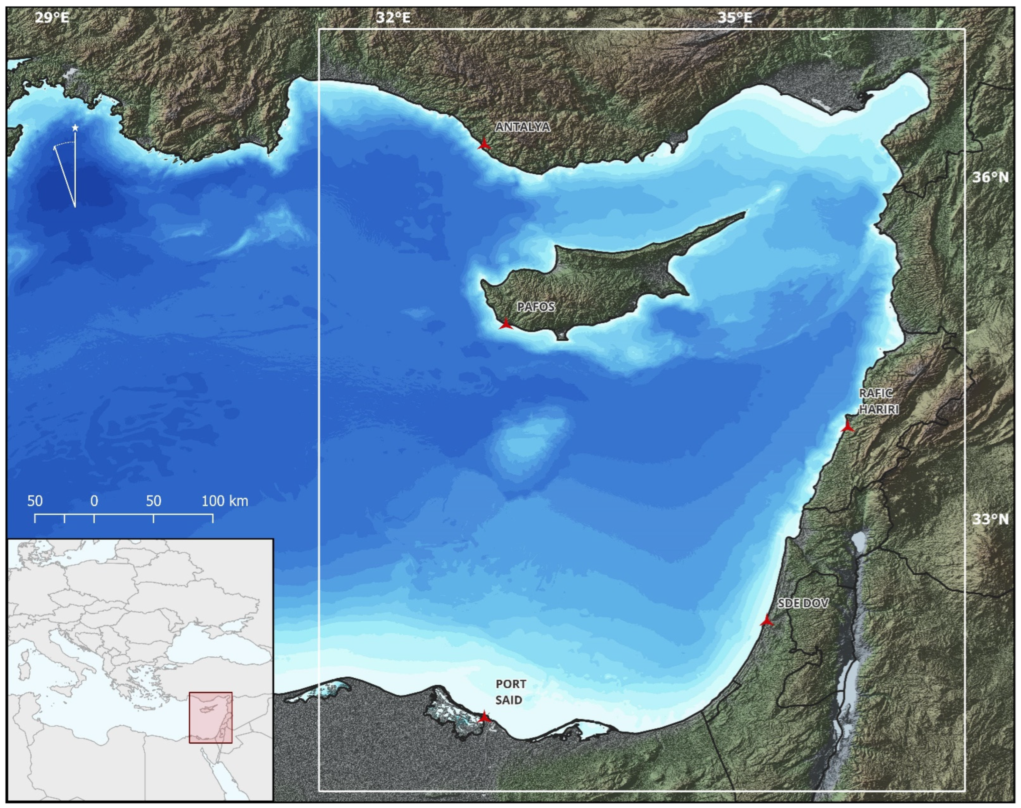
Few datasets are currently of sufficient size and are available at a spatial resolution fine enough to be used for a thorough wind climate characterization over extended areas. This study aims precisely at evaluating four high spatial resolution wind speed datasets (

Table 1. Overview of the numerical datasets.

	MESCAN-SURFEX	CERRA	COSMO-REA6	NEWA
Model	ERA40/ERA-INTERIM	ERA5	COSMO v4.25	Modified WRF V3.8.1
Assimilation system	UERRA-HARMONIE downscaling and optimal interpolation	HARMONIE-ALADIN data assimilation system	Nudging	-
Domain	CORDEX-EUR11	CORDEX-EUR11	CORDEX-EUR11	Europe (10 domains)
Horizontal resolution	~0.050° × 0.050° (5.5 km)	~0.050° × 0.050° (5.5 km)	0.055° × 0.055° (~6 km)	~0.027° × 0.027° (3 km)
Temporal resolution	6 h	3 h	1 h	30 min
Temporal coverage	1961–2019	1984–2021	1995–2019	1989–2018
Vertical levels	14	106	40	61
Reference	[51]	[52]	[36]	[43]

), namely the Uncertainties in Ensembles of Regional Reanalyses System Surface Reanalysis (UERRA MESCAN-SURFEX), the Consortium for Small-scale Modeling regional reanalysis (COSMO-REA6), New European Wind Atlas (NEWA), and Copernicus Regional Reanalysis for Europe (CERRA), against observations from five coastal meteorological stations each located in a different country along the Levantine basin (

Table 2. Meteorological stations information.

		PORT SAID	SDE DOV	RAFIC HARIRI	ANTALYA	PAFOS
Begin Date		1 March 1949	10 May 2004	19 October 1932	10 May 2004	1 January 1949
End Date		Present	30 June 2019	Present	Present	Present
Country		Egypt (EG)	Israel (IS)	Lebanon (LE)	Turkey (TU)	Cyprus (CY)
Latitude		31.27	32.12	33.82	36.30	34.72
Longitude		32.30	34.78	35.49	32.30	32.49
Elevation		6.00	13.00	26.51	28	12.49
Distance to coast		0.010° (~1.11 km)	0.003° (~0.33 km)	0.009° (~0.99 km)	0.027° (~2.99 km)	0.011° (~1.22 km)
Distance to closest node	UERRA	0.010° (~1.11 km)	0.015° (~1.67 km)	0.018° (~2.00 km)	0.029° (~3.22 km)	0.009° (~1.00 km)
	CERRA	0.010° (~1.11 km)	0.015° (~1.67 km)	0.018° (~2.00 km)	0.029° (~3.22 km)	0.009° (~1.00 km)
	COSMO	0.021° (~2.33 km)	0.025° (~2.78 km)	0.025° (~2.78 km)	0.028° (~3.11 km)	0.021° (~2.33 km)
	NEWA	-	-	0.004° (~0.44 km)	0.020° (~2.22 km)	0.015° (~1.67 km)

). An additional element of the originality of this work is that no previous study has attempted to evaluate the above-mentioned products against more accurate observations in the offshore eastern Mediterranean area, either on a decadal or a seasonal time scale. Once evaluated, the above products can provide valid alternatives (to absent or insufficient in situ measurements) for finely resolved wind regime characterizations along the eastern Mediterranean basin, a promising region for future offshore wind farm installations. The statistical analysis is performed using a 10-year wind speed time series from each data source, covering the period between 2009–2018 at multiple temporal scales (i.e., monthly, annual, full decade). The remainder of this paper is structured as follows: Section 2 describes the datasets used in this study and data processing prior to the statistical analysis as well as the methods used for the evaluation. In Section 3, the results of the statistical evaluation are presented while Section 4 and Section 5 are devoted to the discussion and the conclusions, respectively.

2. Data and Methods

2.1. Study Area

The present study focuses on the easternmost part of the Mediterranean Sea as defined by the white outline in Figure 1. The area of interest encloses offshore regions as parts of the exclusive economic zones (EEZ) of five different countries (Egypt, Israel, Lebanon, Turkey, and Cyprus) where individual studies have been conducted for the potential exploitation of clean energy sources. In general, wind fields over eastern Mediterranean exhibit high seasonal variability [53]. The wind climate in the semi-enclosed Levantine basin is subject to regional northerly (Etesian) winds blowing from the Aegean Sea over the summer period [54]. According to [55], these annually reoccurring winds are formed due to the difference in barometric pressure between the Balkans and the Levantine area. Moreover, winds are locally influenced both by the land/sea interactions due to the nearshore topography and steep bathymetry but also by the large island of Cyprus close to the center of the basin [47]. Nevertheless, high depths at relatively short distances from the coast imply reduced cost for the development of wind farm installations in the case of favorable wind conditions. Therefore, gaining insights regarding the wind resource potential over the study area in view of the climate change impacts on the Levantine Sea is timely and critical.

2.2. Gridded Datasets

2.2.1. UERRA MESCAN-SURFER

Reanalysis data for a set of essential climate variables (ECV) have been developed within the context of UERRA project and are delivered by Copernicus Climate Data Store (CDS)—available at https://cds.climate.copernicus.eu. UERRA reanalysis is composed of two systems, namely UERRA-HARMONIE and MESCAN-SURFEX. The first refers to a 3D data assimilation system for regional reanalysis while the latter is a complementary surface reanalysis system forced via optimal interpolation to provide improved 2D analysis. MESCAN-SURFEX wind variable, in particular, is downscaled from UERRA-HARMONIE fields at the spatial resolution of 5.5 km using additional surface observational data [51]. MESCAN-SURFEX is based on MESCAN (MESan and CANari) surface analysis and SURFEX (SURFace EXternalise) land surface model accounting for the fluxes exchange between surface and atmosphere. The temporal coverage of the data is limited by the availability of ERA-Interim global reanalysis which forces UERRA-HARMONIE. Thus, the temporal coverage of MESCAN-SURFEX is from 1961 to 2019, from when the new system (Copernicus Regional Reanalysis for Europe—CERRA) launched in operation mode. The UERRA datasets are available each day every 6 h, starting at 00 UTC and covering the entire European domain.

2.2.2. CERRA

CERRA provides spatially and temporally complete and consistent historical reconstructions of meteorological variables. The single level CERRA subset refers to reanalysis from 1984 to the present for the pan-European domain. The product is provided and delivered by the European Copernicus program in collaboration with the Swedish Meteorological and Hydrological Institute (SMHI), Meteo-France, and the Norwegian Meteorological Institute. CERRA is built upon the combination of remote sensing data and local observations, as well as being forced by the initial and boundary conditions of global ERA5 reanalysis data to downscale model outputs to 5.5 km spatial resolution. Like UERRA, CERRA is based on the HARMONIE-ALADIN data assimilation system, which also applies a 3D variational analysis (3D-VAR) to conduct assimilation every 3 hours. The use of HARMONIE–ALADIN as a numerical weather prediction model makes CERRA an alternative modelling approach for both wind energy and uncertainty modelling [56]. Instantaneous 10 m wind speed values are used in this study. These refer to wind speeds available for each grid point of a Lambert conformal conical grid projection at 10 m above the surface [57].

2.2.3. COSMO-REA6

COSMO-REA6 high-resolution regional reanalysis was developed by Climate Monitoring and Diagnostics group of the Hans-Ertel Centre (HErZ) for Weather Research. COSMO-REA6 is forced by COSMO NWP model, which is part of the operational NWP model chain of the German Meteorological Service (DWD) and uses lateral boundary conditions from ERA-Interim European Centre for Medium-Range Weather Forecasts (ECMWF) global reanalysis. COSMO-REA6 regional atmospheric reanalysis is available for the period between 1996–2019 and stretches across the European CORDEX EUR-11 domain on a rotated latitude–longitude grid and comprises 40 vertical levels. Non-hydrostatic forecast COSMO model combines the NWP forecasts with various observation sources for data assimilation, e.g., aircraft, SYNOP station, buoys, radiosondes, and wind profilers, via a continuous nudging data assimilation scheme [58]. COSMO-REA6 was discontinued in August of 2019 following the end of ERA-Interim operation [53]. COSMO-REA6 2D and 3D fields are archived at https://opendata.dwd.de/climate_environment/REA/COSMO_REA6/ (accessed on 10 April 2024), where hourly wind velocity U and V direction data are available for direct download at the horizontal resolution of 0.055° (approximately 6 km). DWD is already developing a second version of COSMO-REA6 as a continuation of the previous regional reanalysis dataset while COSMO-REA2 is also produced at the horizontal resolution of 0.018°, but only the Central Europe domain [59].

2.2.4. NEWA

NEWA ERANET+ project’s goal was to develop a higher resolved and more accurate wind atlas (compared to the previous European Wind Atlas (EWA)), taking advantage of state-of-the-art technological and scientific improvements. In response to the need to quantitatively assess the wind potential over Europe towards supporting wind energy development, NEWA uniform high-resolution dataset was created and made publicly available at https://map.neweuropeanwindatlas.eu/. NEWA wind statistics over the ocean surface cover 100 km offshore plus the Baltic and the North Seas [60] excluding the offshore area stretching from southern Tunisia to Jordan. A modified version (version 3.8.1) of the Weather Research and Forecast (WRF) model was employed to perform a series of mesoscale simulations over a period of 30 years (1989–2018) in a nested grid of 3 km × 3 km and at 30 min temporal resolution. WRF was forced by ERA5 via dynamical forcing, using spectral nudging above the planetary boundary layer (PBL) to preserve the coherence with large-scale atmospheric patterns. The final product includes wind speed and direction variables at different heights ranging from 10 to 500 m above the ground level (a.g.l). The surface roughness was adjusted based on different land use/cover and terrain data sources [43]. Almost a year after NEWA’s release, ref. [61] attempted to evaluate the product’s wind statistics against data from masts across Europe. Although the study was limited to onshore areas, model quality was proved more than sufficient compared to conventionally used numerical datasets. Further downscaling using the Wind Atlas Analysis and Application Program (WAsP) was employed to reach a horizontal resolution at which local wind flow features can be captured. WAsP linear models and sub-models allow for wind climate conditions extrapolation to nearby sites [62]. The 50 m resolution product, however, is not available for download over a long-term period.

2.3. In Situ Observations

The online hub of National Centers for Environmental Information (NCEI) of the national Oceanic and Atmospheric Administration (NOAA) maintains hourly and sub-hourly observational data of more than 20,000 meteorological stations around the globe. Stations information, including wind speed and direction, can be retrieved via https://www.ncei.noaa.gov/maps/hourly/ (accessed on 3 June 2024). The observational data used in this work are broadcast from five coastal meteorological stations, each located in a different country in the study area (Figure 1). The selection of stations was based on multiple criteria, with the quality of the data time series being the most important. Thus, only stations with more than 90% of good quality data (based on the associated data quality index Q = 1) were chosen to allow comparison between consistent time series. Second, as the comparison aims to evaluate the wind speed numerical datasets towards offshore wind resource potential assessment, in the absence of offshore observational data, meteorological stations were chosen that were relatively close to the coast. The most distant station of those selected is located in Antalya in Turkey, 0.027 degrees (~3 km) away from the coastline. Moreover, the stations chosen were located in a relatively homogeneous and flat terrain to reduce the bias when evaluating the averaged model outputs against point measurements. Last, the data time series should be of sufficient size to cover the period of interest, also matching the numerical datasets described above. Therefore, observational data were acquired between 1 January 2009 and 31 December 2018, although most of the station measurements go back several decades. Wind speed information is associated with a reporting type, according to the World Meteorological Organization’s (WMO) international code forms [63]. Measurements from the meteorological stations used in this study include the following reporting types: surface observations from a fixed land station (FM-12-synop), aerodrome routine meteorological report (FM 15-METAR), aerodrome special meteorological report (FM 16-SPECI), and fully automatic systems report (AUTO). To ensure consistency among in situ measurements obtained from various stations, any duplicated wind speed values were discarded from the time series. Only measurements corresponding to hourly reporting times (:00) were retained, with the exception of Sde Dov and Antalya, where wind speed values are reported only at :50.

2.4. Statistical Evaluation Metrics

This section presents the methods used both for the numerical dataset evaluation against the in situ measurements derived from the meteorological stations and the wind power density preliminary comparison. It should be noted that due to the limited extent of NEWA spatial coverage, no comparison is feasible between NEWA and observations derived from two of the meteorological stations, namely those located at Port Said and Sde Dov. Prior to the wind power density calculation, wind speed values from the extracted time series were extrapolated from 10 m to 100 m a.g.l. to match a typical wind turbine hub height. The following evaluation is decomposed in two phases. The first phase focuses on the long-term statistics over the time periods spanning each dataset, in which the focus is primarily on the temporal distributions of the various datasets with emphasis on their statistical measures. Different time frequencies are also considered to examine and inter-compare wind speed variations. Statistical distributions are also fitted to each time series and the associated parameters are compared. The second phase of the evaluation involves a paired comparison, where in situ measurements are matched with the closest wind speed estimates in time, within a reasonable time threshold. This approach allows for the extraction of mismatch statistics between the co-registered data points.

Due to the inconsistency between models and meteorological stations spatial support (pixels of averaged values vs. points), direct comparison between the referenced datasets is not feasible. While this is a known issue in the related literature [64], no current means are available for mitigating the uncertainty associated with the spatial interpolation often used, let alone a means for including the existence of a dense meteorological station network [65]. Moreover, the fine spatial resolution of the selected datasets further reduces the bias, even though the distance between the station location and the pixel center is not fixed. Therefore, we compared the meteorological station observations with the corresponding value from the numerical dataset pixel that each station falls within.

Commonly used statistical metrics were applied to evaluate the performance of the numerical datasets for modeling the wind speed over a 10-year time period. More specifically, Pearson’s correlation coefficient (R), root mean squared error (RMSE), mean absolute error (MAE), and bias are used as evaluation metrics, while the bias histogram, quantile–quantile (Q-Q plots), and Taylor diagrams [66] are employed to visually depict the deviations among the different datasets of modelled wind speed against in situ measurements. The above metrics and plots are computed both for the full period of interest as well as to quantify the seasonal variations. The boxplots of the numerical datasets and observations were additionally compared over the different seasons.

The equations for the aforementioned statistical metrics are as follows:

$$R={\displaystyle \frac{{\sum }_{i=1}^N(u_i-\overline{u})(v_i-\overline{v})}{\sqrt{{\sum _{i=1}^N(u_i-\stackrel{̿}{u})}^2}\sqrt{{\sum _{i=1}^N(v_i-\stackrel{̿}{v})}^2}}}$$

(1)

$$RMSE=\sqrt{{\displaystyle \frac{1}{N}}{\sum }_{i=1}^N{(u_i-v_i)}^2}$$

(2)

$$MAE={\displaystyle \frac{1}{N}}{\sum }_{i=1}^N\left|u_i-v_i\right|$$

(3)

$$Bias={\displaystyle \frac{1}{N}}{\sum }_{i=1}^N\left(u_i-v_i\right)$$

(4)

where $u_i$ and $v_i$ are the observed and modeled wind speed values and $\stackrel{̿}{u}$ and $\stackrel{̿}{v}$ are the mean observed and modeled wind speeds, respectively. $N$ represents the total number of wind speed values.

Lastly, numerical datasets used in this study present different temporal resolution (Table 1). Therefore, the paired evaluation is based on the extraction of the simultaneous (within a 15 min interval) values of in situ measurements and each of the corresponding pixel values of the numerical datasets. Time steps where no match is found within the aforementioned interval are omitted. The selection of a longer time interval would result in more value pairs although with increased added bias. The resulting 10-year wind speed paired time series were compared via the statistical evaluation methods described in the subsequent sub-sections. Seasonal comparisons were made possible by averaging observations and numerical dataset values in spring (MAM), summer (JJA), autumn (SON), and winter (DJF).

2.5. Extrapolation to Wind Turbine Hub Height

Prior to computing the wind power density at each location, wind speed values need to be vertically extrapolated to match a typical wind turbine hub height (100 m a.g.l.). Several methods have been tested, including more complex (e.g., Monin–Obukhov logarithmic variation [67]) and simplistic (power law [68]) techniques for extrapolating the wind speed values at a desired height. A comprehensive review of the extrapolation models applied for wind energy applications is given in [69,70]. In this work, for the sake of simplicity and given the lack of required measurements (e.g., surface fluxes, friction, friction velocity, etc.), neutral atmospheric stability was assumed; therefore, the logarithmic wind profile is preferred for the vertical extrapolation of the observed and modelled wind speed values [71], defined as follows:

$$u_{\left(z_r\right)}={\displaystyle \frac{\mathrm{l}\mathrm{n}\left(\frac{z_r}{z_0}\right)}{\mathrm{l}\mathrm{n}\left(\frac{z}{z_0}\right)}}{u}_{\left(z\right)}$$

(5)

where $u_{\left(z_r\right)}$ the wind speed at the reference height ($m/s$), $u_{\left(z\right)}$ is the wind speed at height $z\left({\displaystyle \raisebox{1ex}{$m$}\!\left/ \!\raisebox{-1ex}{$s$}\right.}\right)$ and $z_0$ is the surface roughness, set to 0.03 m which corresponds to open areas according to the values given in [72].

2.6. Weibull Probability Density Functions (PDFs)

To compute the wind power density output in a given grid cell or domain, one needs to model the empirical wind speed distribution first. the Weibull probability density functions (PDFs) are typically used to model the positively skewed distribution of wind speed data over time. Although various alternatives for modeling the wind speed frequency distributions also exist (e.g., gamma, lognormal), Weibull has been widely used for wind energy applications, especially on relatively flat terrain/surfaces [73]. The theoretical Weibull PDF is expressed as:

$$f\left(u\right)={\left({\displaystyle \frac{k}{\lambda }}\right)\left({\displaystyle \frac{u}{\lambda }}\right)}^{k-1}\exp \left[{-\left({\displaystyle \frac{u}{\lambda }}\right)}^k\right],u,k,\lambda >0$$

(6)

where $u$ is the wind speed, and k and λ the shape and scale parameters, respectively. While k accounts for the overall form, including the skewness of the distribution, λ determines the peak–width ratio, also adjusting the width of the distribution. A k value equal to 3.6, for example, largely resembles the Gaussian distribution, while for a given value of k, the distribution flattens out as λ increases. The estimation of Weibull shape and scale parameters, and model fitting by extension, involves some measure of probability agreement between the model and sample statistics. Here, the maximum likelihood method (MLM) is used to maximize this convergence as it has demonstrated good performance in parameter estimation in past studies [74,75].

2.7. Wind Power Density

Wind turbine power curves are commonly utilized, and therefore widely employed, for predicting the power generation of a wind turbine. Nevertheless, during the phase of resource assessment, when the specific traits of the wind resource are still undetermined, an efficient indicator of wind power can be derived through wind power density. Wind power density, denoted as P, represents a conventional measure in wind resource assessment studies, indicating the amount of kinetic energy passing through a unit of surface per time unit (typically expressed in W/m²) [76]. The wind power density can be directly computed from the wind speed time series as:

$$P_{\left(U\right)}=0.5\rho {\displaystyle \frac{1}{{\rm N}}}\sum _{i=1}^N{U}_i^3$$

(7)

where ρ is the air density (1.225 kg/m³) at standard atmospheric condition (i.e., average atmospheric pressure at sea level and temperature of 15 °C) and $U_i$ is the wind speed. P is also expressed in terms of the Weibull PDF shape and scale parameters as:

$$P_w=0.5\rho \underset{0}{\overset{\infty }{\int }}{U}^{3}f(U;k,\lambda )dU=0.5\rho k^3\Gamma \left(1+{\displaystyle \frac{3}{\lambda }}\right)$$

(8)

Here, wind power density is calculated by applying Equation (8) after fitting Weibull distributions to each node wind speed time series.

3. Results

This section details the results from applying the statistical evaluation metrics described earlier and includes an analysis of wind power density derived from Weibull parameters for both observational and numerical datasets. The statistical comparison is divided into two parts: a time series comparison, which assesses the full range of wind speed values across each dataset over time, and a paired comparison, which focuses on wind speed values recorded within a specified time window of each other. This dual approach provides a comprehensive evaluation of dataset performance, revealing discrepancies and assessing the reliability of wind speed estimates for potential wind resource assessments.

3.1. Wind Speed Time Series Statistical Comparison

After adjusting the modeled wind speed data to the height of the meteorological stations, a statistical comparison was conducted between coastal meteorological observations, used as a reference, and wind speed values from the nearest UERRA, CERRA, COSMO-REA6, and NEWA nodes. The summary statistics for the described data are presented in

Table 3. Summary statistics of wind speed data from five meteorological stations and the nearest UERRA, CERRA, COSMO-REA6, and NEWA nodes.

PORT SAID
Dataset	No. of Data	Min	Max	Mean	Median	Std	IQR	90th Pctl.
Station	83.983	0.50	29.30	4.29	4.10	1.91	2.00	6.70
UERRA	14.608	0.17	16.81	5.02	4.86	2.06	2.48	7.58
CERRA	29.216	0.02	18.68	4.93	4.77	2.17	2.87	7.66
COSMO	87.648	0.06	19.60	5.21	5.02	2.32	3.04	8.18
NEWA	-	-	-	-	-	-	-	-
SDE DOV
Dataset	No. of Data	Min	Max	Mean	Median	Std	IQR	90th Pctl.
Station	57.438	0.50	26.20	4.10	3.60	2.03	2.50	6.20
UERRA	14.608	0.03	17.18	3.44	3.09	2.01	2.77	5.78
CERRA	29.216	0.01	18.70	3.60	3.36	2.05	2.44	5.92
COSMO	87.648	0.01	12.60	2.24	1.87	1.36	1.84	4.21
NEWA	-	-	-	-	-	-	-	-
RAFIC HARIRI
Dataset	No. of Data	Min	Max	Mean	Median	Std	IQR	90th Pctl.
Station	77.275	0.50	19.60	3.21	2.60	1.91	2.00	5.70
UERRA	14.608	0.02	10.46	2.12	1.97	1.29	1.86	3.71
CERRA	29.216	0.03	16.97	3.26	2.93	1.89	2.20	5.72
COSMO	87.648	0.01	14.70	2.51	2.19	1.52	1.88	4.55
NEWA	175.243	0.00	23.36	3.63	3.08	2.34	2.31	6.58
ANTALYA
Dataset	No. of Data	Min	Max	Mean	Median	Std	IQR	90th Pctl.
Station	49.315	0.50	17.00	2.73	2.60	1.44	2.10	4.60
UERRA	14.608	0.01	9.83	1.56	1.33	1.09	1.57	2.96
CERRA	29.216	0.02	10.71	2.16	2.03	1.14	1.41	3.47
COSMO	87.648	0.01	9.68	1.66	1.50	0.93	1.06	2.82
NEWA	175.243	0.00	25.22	3.44	3.07	1.97	1.68	5.35
PAFOS
Dataset	No. of Data	Min	Max	Mean	Median	Std	IQR	90th Pctl.
Station	71.231	0.00	18.50	3.96	3.60	2.00	2.50	6.70
UERRA	14.608	0.01	11.84	2.49	2.07	1.54	2.03	4.60
CERRA	29.216	0.03	15.47	3.57	3.28	1.84	2.24	5.98
COSMO	87.648	0.02	13.61	2.92	2.58	1.64	1.86	5.14
NEWA	175.241	0.00	18.96	4.23	3.81	2.07	2.31	7.10

. It is important to note that in this initial evaluation, the entire time series from each data source was utilized to assess the overall performance of the modeled wind speed estimates in relation to long-term observational data. Although there is a significant difference in the number of observations among the datasets, the analysis provides valuable insights that can also be leveraged for a preliminary offshore wind resource assessment.

The extended time series available from in situ measurements and NEWA wind speed estimates, which benefit from a higher temporal reporting frequency, reveal a broader range of wind speeds and more extreme values compared to the more limited wind speed samples from other numerical datasets. This broader range and higher extremes (more evident in the boxplots in Figure 2) are particularly evident in the maximum wind speed values recorded at the five meteorological stations. For instance, at Port Said and Sde Dov, the observed maximum wind speeds of 29.30 m/s and 26.20 m/s, respectively, are significantly higher than those reported by the other datasets. Conversely, the outliers in the UERRA, CERRA, and COSMO-REA6 datasets extend over a shorter range above the upper whisker. Consequently, modeled wind speed values, except for NEWA, are generally limited to below 20 m/s at all locations, with little variation in maximum values between the datasets.

Across all locations, station data generally show higher maximum wind speeds compared to the modeled datasets, suggesting that the models may underestimate extreme wind values. Additionally, NEWA data tend to show higher mean wind speeds compared to the other datasets and, in some cases, even exceed the mean wind speeds observed at the meteorological stations. This indicates a possible tendency for the NEWA dataset to overestimate average wind speeds. Overall, while the observational data demonstrate greater extremes and variability, the modeled datasets, particularly excluding NEWA, appear to have limitations in capturing extreme wind events and may exhibit biases in estimating average wind speeds.

As expected, due to the asymmetric nature of wind distributions, the mean wind speed values are higher than the medians. Both the mean and the median are higher for the observational and NEWA data at every location except Port Said. The largest divergence is observed at Antalya, where the mean of observations and all modeled wind speed values differ by more than 0.5 m/s, and the difference between NEWA and other numerical datasets exceeds 1 m/s. Given the skewed distributions typical of wind speed time series, the median is a better indicator of the average wind speed. This is particularly relevant here, as the observational and NEWA data exhibit a broader range of outliers compared to other datasets. Additionally, the inherent scale and support of each dataset play a crucial role in the presence and extent of outliers, further influencing the interpretation of wind speed statistics. Evidently, wind speed patterns in the northern offshore area of the eastern Mediterranean near the Antalya meteorological station tend to differ from those in the southern and western areas. This distinction is indicated by the tendency for wind speeds to become more intense moving southward, with Pafos’ statistics falling in an intermediate zone relative to its location. This is likely due to the influence of the Cyprus mainland on the winds blowing eastward from the Mediterranean Sea. Comparing the median values of observational and numerical data provides a clear indication of local wind speed variations. Similar observations are made when examining the standard deviation of the datasets, with less variability in the northern areas and greater variability in the southern areas.

Figure 2 shows the interquartile range (IQR), which is defined as the difference between the 75th and 25th percentiles, or the box length as shown in the relevant subfigures. Considering this, we can observe that while both the standard deviation and the IQR of observational data at Antalya and Paphos present a relatively equal difference from the corresponding statistics of the modeled wind speed datasets, this gradually changes moving southward. Eventually, both statistics are higher for the modeled data at Port Said. This indicates that the models introduce greater variability in wind speed estimates in the southern regions than what is observed in the reference data.

When comparing the datasets, it is evident that NEWA and COSMO frequently exhibit higher standard deviations and IQRs than the station data, indicating greater variability in their wind speed estimates. This suggests that these models may be more adept at capturing fluctuations in wind speeds. However, they may still fall short in accurately representing extreme values, as evidenced by the 90th percentile values.

Boxplots in Figure 2 clearly illustrate that observational data and NEWA wind speed values exhibit a broader range and greater variability, particularly in the northern regions around Antalya and Paphos. This expanded range is most pronounced at these locations compared to the other datasets. COSMO-REA6 also shows a relatively wide IQR, though this is less apparent at Port Said. It is important to highlight that the higher number of outliers in the in situ measurements and NEWA is due to their higher temporal resolution, which captures more variability than the coarser temporal resolution of the other numerical datasets. Consequently, the station data in these locations exhibit a wider range of values. In contrast, UERRA, CERRA, and COSMO-REA6 datasets, while extensive in time series length, demonstrate a more restricted value range with outliers predominantly clustered near the upper whiskers. This indicates that despite the broad coverage of these datasets, they may not fully capture the extreme wind speeds observed in the observational data and NEWA. The differences between modelled and observed wind speeds vary by location, with models generally performing better in some areas (e.g., capturing variability) but not as well in others (e.g., extreme values).

Figure 3 illustrates the annual, monthly, and hourly cycles of the average observed and estimated wind speeds at the five coastal meteorological station locations. This plot is particularly useful for analyzing wind speed variations over different time intervals and identifying potential trends across various datasets. Such insights are crucial for understanding intermittent wind patterns, calculating loads on wind turbines, and ultimately aiding in accurate reliability assessments and the development of cost-effective wind energy solutions. According to Figure 3, no significant annual trends are observed in either the measured or modeled wind speeds, with values generally fluctuating between 2 and 4 m/s at most locations. An exception is noted at Port Said, where average wind speeds cluster around 5 m/s. The most significant deviations occur at Sde Dov, where model outputs, particularly those from COSMO, underestimate the observed wind speed by approximately 2 m/s on average. Although NEWA data are available only for Rafic Hariri, Antalya, and Pafos, they follow a trend similar to the observational data, whereas those from UERRA and COSMO show the greatest discrepancies. Notably, except for Port Said, model wind speed outputs consistently underestimate the average observed wind speeds at all locations.

Similar variations are observed across the various locations and data sources on a seasonal scale. A general trend of slightly increasing average wind speed is evident during the winter months, while the lowest average wind speeds typically occur in April during spring and between October and November during autumn, depending on the dataset. The Rafic Hariri and Antalya regions exhibit the most pronounced seasonality, with wind speeds exceeding 4.5 m/s in winter and dropping below 2 m/s during the summer months. This may be partly attributed to local flow conditions influenced by the prominent landmass extending from Cyprus mainland toward the south. While CERRA and NEWA generally align with in situ measurements—with Antalya being a notable exception—UERRA and COSMO display distinct intra-annual variability patterns across the study locations. High-intensity and stable wind speeds of approximately 6 m/s are observed year-round at Port Said, decreasing to below 3 m/s further north. Intermediate local minima and maxima are observed between March and April and October and November. At Sde Dov, COSMO shows a stable average wind speed of 2 m/s, which deviates significantly from the other datasets.

The limited temporal resolution of UERRA and CERRA, with only four and eight daily wind speed estimates (6 h and 3 h intervals, respectively), clearly impacts their average wind speed variations, particularly on finer temporal scales. These datasets may not capture peak and minimum wind speeds as accurately as observational data. The hourly variations, presented in the last column of Figure 3, reveal a clear peak in wind speed around noon, except at Port Said, where the highest wind speed values are shifted by 1–2 h into the afternoon. Discontinuities observed in the data for Rafic Hariri, occurring every 3 h starting from 00:00, suggest a possible acquisition or reporting issue. Although these values may not be considered accurate, the overall trend remains consistent when considering variations in the other datasets.

Finally, overestimations of observed wind speeds are evident in the UERRA, CERRA, and COSMO datasets at Port Said, with this overestimation becoming more pronounced further north. In contrast, NEWA seems to follow the wind speed temporal trends closely, with the exception of early morning and late afternoon data at Antalya. Nevertheless, no significant deviations are observed among the four datasets across most locations of interest and at various temporal scales. The seasonal variability, more pronounced at stations in the northern part of the study area, may be attributed to the notable differences between diurnal and nocturnal wind speed values. Additionally, the northern coasts of the eastern Mediterranean generally exhibit reduced diurnal variation compared to the southern coasts, where increased nocturnal wind speeds and decreased meridional velocities are more common [77]. For example, Cyprus’s southern coast is characterized by intense diurnal variations, with average midday wind speeds ranging from 5.5 to 6 m/s, compared to nighttime values of 2.5 to 3 m/s. However, as the year progresses toward summer, average wind speeds gradually decrease during the evening hours due to generally milder atmospheric circulation and reach their peak during midday, with values as high as 8 m/s on average. This persistent diurnal pattern, coupled with strong seasonal and time-of-day variations, significantly influences the wind flow conditions in the area and must be carefully considered in any wind farm planning project [78].

3.2. Paired Comparison

As indicated in the previous section, the sampling rate varies significantly between the three data sources. At Pafos for example, the 83,983 meteorological station wind speed data observations were obtained for the time period between 1 January 2009 and 31 December 2018, yet only 14,608 UERRA and 29,216 CERRA data values are available for the same time interval. As previous analysis did not account for this inconsistency, a paired comparison analysis is also performed to allow fair statistical comparison. In this section, the same number of data for each location are considered by limiting the time series to dates and times where all data sources match. The number of samples is therefore limited by the dataset with the lowest temporal resolution, which in this case is UERRA. To address the discrepancy caused by the difference in data acquisition times at the Sde Dov and Antalya locations (where stations report at :50), a 15 min search window is applied to these sites. In general, the exclusion of these values from the station time series has led to a decrease in the paired sample size yet high enough to allow for a match-up comparison within the time period of interest. In what follows, commonly used statistical metrics are applied to evaluate the performance of the model outputs. More specifically, Pearson’s correlation coefficient (R), root mean squared error (RMSE), mean absolute error (MAE), and bias are used as evaluation metrics while quantile–quantile (Q-Q) plots and Taylor diagrams [67] are employed to visually depict the deviations among the different datasets of modelled wind speed against in situ measurements. The number of pairs are compared and the mismatch statistics of the paired comparison are summarized in

Table 4. Mismatch statistics of paired wind speed data from five meteorological stations and the nearest UERRA, CERRA, COSMO-REA6, and NEWA nodes.

	Port Said				Sde Dov
Dataset	R	RMSE	MAE	Bias	R	RMSE	MAE	Bias
UERRA	0.70	1.71	1.29	0.71	0.78	1.33	1.00	−0.09
CERRA	0.73	1.63	1.23	0.65	0.79	1.31	0.98	0.03
COSMO	0.68	2.01	1.55	0.99	0.66	2.11	1.59	−1.42
NEWA	-	-	-	-	-	-	-	-
	Rafic Hariri				Antalya
Dataset	R	RMSE	MAE	Bias	R	RMSE	MAE	Bias
UERRA	0.54	1.48	1.10	−0.41	0.62	1.52	1.22	−0.97
CERRA	0.68	1.60	1.20	0.73	0.60	1.28	0.93	−0.43
COSMO	0.52	1.53	1.13	0.01	0.41	1.66	1.24	−0.93
NEWA	0.59	2.23	1.56	1.11	0.40	2.04	0.74	0.69
	Pafos
Dataset	R	RMSE	MAE	Bias
UERRA	0.72	1.94	1.57	−1.36
CERRA	0.75	1.39	1.09	−0.30
COSMO	0.48	2.08	1.63	−0.90
NEWA	0.66	1.68	1.24	0.30

No. of pairs: Port Said: 14,265; Sde Dov: 9714; Rafic Hariri: 13,523; Antalya: 8083; Pafos: 8117.

.

The performance of the four reanalysis datasets—UERRA, CERRA, COSMO, and NEWA—varies significantly across the five locations, as shown by the statistical metrics derived from the paired comparison. CERRA consistently demonstrates superior performance, with the highest R values, ranging from 0.60 at Antalya to 0.79 at Sde Dov, and the lowest RMSE and MAE values. For example, at Pafos, CERRA achieves an R value of 0.75 and an RMSE of 1.39 m/s, significantly outperforming COSMO, which has an R of 0.48 and an RMSE of 2.08 m/s. The bias values also indicate that CERRA generally has lower absolute bias, reflecting more accurate wind speed predictions.

The impact of sample size on the statistical metrics is evident across the datasets. At Port Said (14,265 pairs) and Rafic Hariri (13,253 pairs), for instance, the statistical metrics show more consistent results, with CERRA maintaining high R values and low RMSE and MAE. In contrast, smaller sample sizes, like those at Antalya and Pafos, result in higher variability in the performance metrics. For example, in Antalya, the reduced sample size contributes to a lower R value of 0.62 for UERRA and an increased RMSE of 1.52 m/s, compared to Port Said where UERRA has an R of 0.70 and an RMSE of 1.71 m/s.

NEWA’s high temporal resolution initially allowed it to achieve superior performance in full time series comparisons. However, to match the sample sizes for paired comparisons, the temporal resolution was reduced. This adjustment affected NEWA’s performance, as evidenced by its lower R values and higher MAE in this analysis compared to its earlier performance. For example, at Antalya, NEWA shows a reduced R value of 0.40 and an MAE of 1.24 m/s, which is less favorable compared to its earlier results and CERRA’s current performance. Bias values across datasets also reflect the influence of sample size. UERRA at Rafic Hariri shows a negative bias of −0.41, while CERRA at Port Said has a positive bias of 0.65. COSMO’s performance, marked by high RMSE and MAE and pronounced negative biases at locations such as Pafos, highlights the dataset’s reduced accuracy and consistency. Despite these issues, NEWA still outperforms COSMO in several instances, indicating that while CERRA and UERRA generally offer more reliable wind speed estimations, careful consideration of both sample size and temporal resolution is crucial for accurate wind modeling and prediction. A general linear relationship can be inferred from the correlation coefficients and Q-Q plots presented in Figure 4 for most locations and datasets.

These plots highlight the agreement (or lack thereof) between observed and estimated wind speeds across different quantiles, offering insights into how well each model performs across the spectrum of wind speed conditions. Port Said, with its relatively large sample size of 14,265 pairs, shows a strong alignment between the observed and estimated wind speeds across all quantiles, with the points closely following the 1:1 reference line. This indicates that the reanalysis datasets, particularly CERRA, provide reliable wind speed estimates for this location across both lower and higher quantiles. The consistency across quantiles suggests that these models can accurately capture the entire range of wind speeds at Port Said, making them suitable for various applications in this region. In contrast, Sde Dov, Rafic Hariri, and Pafos demonstrate a pattern where the reanalysis datasets tend to underestimate higher wind speed quantiles. This systematic underestimation is most pronounced in the upper quantiles, where the models consistently predict lower wind speeds than those observed, indicating a potential limitation in capturing extreme wind events. Despite these biases, CERRA generally performs better than the other models, showing closer alignment with the observed data, although some discrepancies remain, particularly at higher wind speeds.

Antalya presents the most significant challenges, as evidenced by its QQ plot. The reanalysis datasets tend to overestimate wind speeds at lower quantiles and underestimate them at higher quantiles, leading to substantial deviations from the 1:1 reference line. This pattern suggests that the models may not adequately represent the wind speed distribution in Antalya, particularly in capturing the extremes. The reduced sample size at Antalya (8083 pairs) further exacerbates this issue, contributing to the observed variability in model performance. COSMO-REA6, in particular, shows noticeable discrepancies across most locations. It consistently displays higher deviations from the 1:1 line compared to UERRA and CERRA, especially in the higher quantiles. This suggests that COSMO tends to struggle with accurately capturing extreme wind speeds, leading to higher RMSE and MAE values, as reflected in the previous analysis. In locations like Pafos and Sde Dov, where wind patterns may be more complex or data are less abundant, COSMO’s performance appears to be less reliable, often underestimating higher wind speeds. NEWA demonstrates varied performance in the QQ plots. At locations like Antalya, NEWA tends to overestimate lower quantiles and underestimate higher quantiles, similar to other reanalysis datasets but often with more pronounced deviations. The need to reduce NEWA’s temporal resolution for paired comparisons also impacted its performance, leading to lower correlation coefficients and increased errors. Despite these challenges, NEWA still outperforms COSMO in several instances, particularly in mid-range quantiles, indicating that while it faces similar issues with extreme wind speeds, it remains competitive with other datasets in certain scenarios.

Overall, the QQ plots reveal that while reanalysis datasets like CERRA and UERRA perform reasonably well in certain locations, such as Port Said, their accuracy diminishes in others, particularly in capturing higher wind speeds and extreme events. COSMO-REA6, in particular, struggles with accuracy across different quantiles, often underestimating extremes. Meanwhile, NEWA, despite its high temporal resolution, shows varied performance depending on location and sample size, suggesting that while it can be effective, it also requires careful consideration in its application.

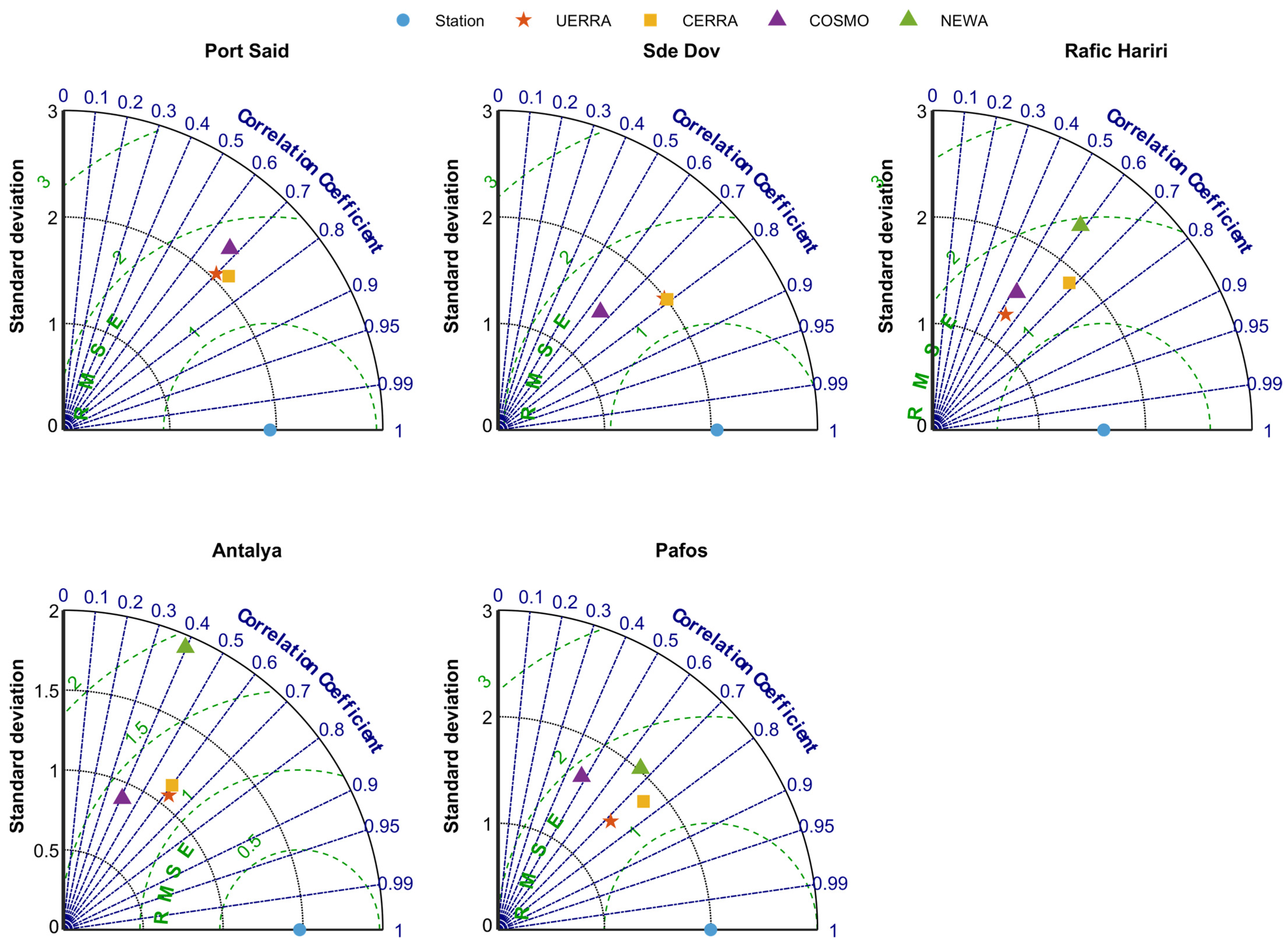
Statistical metrics referenced in this section, namely standard deviation, Pearson’s correlation coefficient, and root mean square error/deviation are also employed to construct the Taylor diagrams at each location (Figure 5); a graph summarizes the skill of the modelled/estimated data to match the spatiotemporal patterns of observations. RMSE can be decomposed into the bias and the centered root mean square error (CRMSE). While the mean error over the datasets in comparison is computed by the bias, the remaining random error is measured by the CRMSE, with the latter being used to construct the Taylor diagram and expressed as:

$$CRMSE=\sqrt{{\displaystyle \frac{\sum _{i=1}^N{\left(\left(u_i-\overline{u}\right)-\left(v_i-\overline{v}\right)\right)}^2}{N}}}$$

(9)

where $u$ and $v$ are the reference and modelled/estimated wind speed values and $N$ is the total number of observations.

From the diagrams, it is clear that CERRA generally outperforms the other datasets, consistently showing high correlation coefficients and standard deviations that closely align with those of the observed data. This confirms that CERRA not only aligns well with observed wind speeds but also accurately reflects the variability in these speeds. UERRA, while slightly less precise, still shows strong correlations and reasonable CRMSE, making it a dependable alternative. COSMO-REA6, on the other hand, demonstrates significant deviations from the observed data. The Taylor diagrams reveal that COSMO-REA6 often fails to capture the full range of wind speed variability, with lower correlation coefficients and higher CRMSE values. This underperformance suggests that COSMO-REA6 is less capable of accurately modeling the complex wind patterns observed at some locations, particularly in regions with more extreme or variable wind speeds. NEWA, when included in the Taylor diagrams, shows varying levels of accuracy. In some locations, NEWA aligns well with observed data, particularly in capturing wind speed variability, but it also exhibits higher CRMSE in certain instances, reflecting challenges in accurately estimating wind speeds, especially when its temporal resolution is adjusted to match the other datasets.

Overall, the Taylor diagrams indicate that CERRA and UERRA are generally the most reliable datasets for wind speed estimation. However, the choice of dataset should be tailored to specific locations, as unique wind characteristics can influence the accuracy of each model. COSMO-REA6 appears to be less effective, especially in regions with complex wind patterns, while NEWA shows promise but requires careful consideration depending on the specific application and location.

The performance of reanalysis and numerical datasets, however, is not consistent across all studies. Variations are often driven by the study area, temporal resolution, scale of comparison, and the specific reanalysis product used. For instance, similar statistics were observed in [79] when comparing several reanalyses of daily wind speed observations from the Integrated Surface Hourly (ISH) dataset, whereas in [80,81], results varied significantly depending on the study area. This underscores the importance of context-specific evaluations when selecting reanalysis datasets for wind speed modeling.

3.3. Weibull Distribution Fitting

Wind potential estimation goes through distribution fitting using a probability distribution that wind speed time series are known to follow. Figure 6 are fitted to the 10-year wind speed time series from each source and are depicted against meteorological station observations empirical probability distribution. The next step is to determine the Weibull distribution’s shape and scale parameters that best match the observed data, in this case using the maximum likelihood estimation. The probability density function (PDF) and cumulative distribution function (CDF) of the Weibull distribution can then be derived using these parameters.

The Station Weibull distribution generally provides a reliable fit to the observed data, effectively capturing the main features of the wind speed distributions. The model-derived distributions, on the other hand, exhibit varying levels of agreement with the station data. The UERRA Weibull distribution shows significant deviations, particularly at Antalya, Rafic Hariri, and Pafos, where it consistently overestimates lower wind speeds and fails to capture the correct peak and shape of the distributions. A similar pattern is observed with the COSMO Weibull distribution, indicating reduced reliability, especially in regions like Sde Dov and Antalya. Conversely, the NEWA Weibull distribution, where available, shows strong agreement with both the observed data and the Station Weibull distribution, particularly at Rafic Hariri and Pafos, suggesting it is better suited for replicating wind speed distributions in these areas. Overall, the analysis suggests that while UERRA and COSMO struggle with significant deviations across multiple locations, NEWA offers a closer fit to the observed data where available. The CERRA Weibull distribution shows mixed performance; for example, it closely matches the observational data and the Station Weibull distribution at Rafic Hariri but shows significant deviations in Antalya. This variability underscores the importance of selecting an appropriate model for accurate wind speed representation, depending on the specific location.

Figure 7 presents a visual comparison of Weibull-derived statistics as a function of the distance from each station to the nearest model node. However, there is no clear evidence that either the Weibull-derived mean or the standard deviation is dependent on distance.

What stands out is the general agreement between the station data and the model-derived standard deviations, in contrast to the mean values, which vary depending on the dataset and location. UERRA and CERRA tend to overestimate the station Weibull-derived means in the southern regions, leading to an underestimation as one moves further north. NEWA closely aligns with the observational data, though with a slight overestimation in both Weibull-derived statistics. Conversely, COSMO-REA6 appears unstable across the locations of interest, with a tendency to underestimate the Weibull-derived statistics compared to the station data. The most significant deviations are observed at Antalya, where all datasets, except for NEWA, underestimate both the mean and standard deviation of the station-derived statistics by more than 1 m/s. Overall, across most locations, the model-derived Weibull wind speed statistics correlate well with the observational data

3.4. Wind Power Density Estimation

Wind resource assessment is critical in the development of offshore wind energy projects. It involves evaluating the wind conditions at potential offshore sites to determine their suitability for installing and operating wind turbines. Accurate assessment ensures the optimal design and successful operation of offshore wind farms, contributing to the growth of renewable energy. Wind resource assessment typically undergoes several stages until a decision regarding the feasibility of developing such a project is made. The initial stage for identifying and evaluating potential sites is referred to as prospecting. This stage involves using wind data based on coarse-scale numerical weather prediction models and reanalysis data to preliminary assess the wind resource, typically on the basis of the annual energy production (AEP). This first-stage evaluation narrows down the number of potential candidate areas to a few promising regions which will be further considered for the subsequent site assessment. Therefore, the present section provides an initial estimate of the wind power density estimated per location and numerical dataset as compared to the corresponding output from the coastal meteorological stations.

As the typical offshore wind turbine hub height is close to 100 m above surface, wind speed values are extrapolated to the above-mentioned height using Equation (5) in order to estimate the wind power density. Therefore, as of this point, the 100 m will be the reference height for wind energy as presented in the rest of this section. Wind power density was calculated by applying Equation (8) after fitting Weibull distributions to the wind speed time series corresponding to each dataset. The seasonal and diurnal WPD were computed to evaluate possible variations.

In general, UERRA and CERRA tend to overestimate WPD, with values often exceeding the observed data by significant margins. For example, at Port Said, UERRA and CERRA both estimate WPD at 212.78 W/m², which is about 48% higher than the observed value of 143.36 W/m². This pattern of overestimation is consistent across other locations, though the degree varies, with CERRA generally providing closer estimates in moderate wind speed regions.

In contrast, COSMO-REA6 frequently underestimates WPD, particularly in areas with complex wind regimes. For instance, at Sde Dov, COSMO-REA6 reports a WPD of just 27.50 W/m², which is approximately 80% lower than the observed 136.44 W/m². However, in some high wind locations, COSMO-REA6 overestimates WPD, such as at Port Said, where it reports 253.23 W/m²—significantly higher than the observed value, highlighting the model’s inconsistency across different environments.

NEWA, although available for fewer stations, generally provides WPD estimates that are closer to the observed values. For example, at Pafos, NEWA estimates WPD at 148.25 W/m², about 19% higher than the observed 124.91 W/m², suggesting a better alignment with the reference values compared to other models. These intercomparisons underscore the importance of carefully selecting models based on specific regional characteristics, as the accuracy of WPD estimates can vary significantly depending on the location and the model used. The findings suggest that no single model consistently outperforms others across all locations, highlighting the need for a tailored approach to wind energy assessment in the eastern Mediterranean.

Table 5. Fitted Weibull parameters and WPD (W/m²) for five meteorological stations and the nearest UERRA, CERRA, COSMO-REA6, and NEWA nodes.

	Port Said			Sde Dov
Dataset	Scale (λ)	Shape (κ)	WPD	Scale (λ)	Shape (κ)	WPD
Station	4.84	2.37	143.36	4.64	2.13	136.44
UERRA	5.64	2.56	212.78	3.88	1.80	96.07
CERRA	5.56	2.40	212.77	4.06	1.85	106.34
COSMO	5.87	2.37	253.23	2.52	1.74	27.50
NEWA	-	-	-	-	-	-
	Rafic Hariri			Antalya
Dataset	Scale (λ)	Shape (κ)	WPD	Scale (λ)	Shape (κ)	WPD
Station	3.63	1.81	78.31	3.09	2.01	42.53
UERRA	2.37	1.69	23.92	1.73	1.50	11.53
CERRA	3.67	1.82	80.44	2.44	1.99	21.20
COSMO	2.83	1.74	38.68	1.87	1.89	10.14
NEWA	4.08	1.67	124.38	3.88	1.85	92.69
	Pafos
Dataset	Scale (λ)	Shape (κ)	WPD
Station	4.49	2.10	124.91
UERRA	2.81	1.73	38.66
CERRA	4.04	2.05	93.51
COSMO	3.30	1.89	55.70
NEWA	4.78	2.14	148.25

highlights significant variability in the performance of numerical models across different locations, with notable intercomparisons between the datasets. In general, UERRA and CERRA tend to overestimate WPD, with values often exceeding the observed data by significant margins. For example, at Port Said, UERRA and CERRA both estimate WPD at 212.78 W/m², which is about 48% higher than the observed value of 143.36 W/m². This pattern of overestimation is consistent across other locations, though the degree varies, with CERRA generally providing closer estimates in moderate wind speed regions.

Table 6. WPD (W/m²) per season for five meteorological stations and the nearest UERRA, CERRA, COSMO-REA6, and NEWA nodes.

	Port Said				Sde Dov
Dataset	Winter	Spring	Summer	Autumn	Winter	Spring	Summer	Autumn
Station	163.90	185.05	122.08	111.78	238.03	151.76	96.90	104.37
UERRA	305.66	232.69	154.62	166.02	169.79	100.15	62.99	72.52
CERRA	299.87	237.23	161.98	161.11	208.09	112.08	56.44	82.71
COSMO	341.32	245.64	197.12	238.14	34.32	31.50	27.14	21.50
NEWA	-	-	-	-	-	-	-	-
	Rafic Hariri				Antalya
Dataset	Winter	Spring	Summer	Autumn	Winter	Spring	Summer	Autumn
Station	130.72	99.42	69.34	52.00	56.62	45.08	45.65	36.72
UERRA	42.34	23.86	13.33	16.88	19.45	9.18	8.34	10.71
CERRA	137.69	94.06	60.69	49.90	35.05	19.53	15.82	18.76
COSMO	54.38	49.51	27.84	31.67	14.07	11.38	9.27	8.86
NEWA	274.33	147.77	63.01	84.02	226.35	87.04	41.54	80.55
	Pafos
Dataset	Winter	Spring	Summer	Autumn
Station	169.25	137.34	113.39	105.00
UERRA	63.45	43.27	29.87	27.43
CERRA	148.55	101.86	70.90	67.19
COSMO	83.38	74.91	40.16	38.59
NEWA	237.88	166.37	101.18	108.86

provides a seasonal comparison of WPD, showing significant variability across different locations and datasets, reflecting the diverse wind regimes in the eastern Mediterranean basin. The data reveal notable differences in WPD across seasons and between the different numerical datasets when compared to observational data. The winter season consistently shows the highest WPD values across all stations, underscoring the season’s importance for wind energy generation. For example, at Port Said, the observed WPD during winter is 163.90 W/m², but the numerical models, particularly UERRA and CERRA, significantly overestimate this value, reporting 305.66 W/m² and 299.87 W/m², respectively. This trend of overestimation persists in other seasons, though to a lesser extent, highlighting a systematic bias in these models that could lead to overestimated wind energy potential if not carefully calibrated.

At Sde Dov, the observed WPD during winter is 238.03 W/m², which is again overestimated by the models, with CERRA providing a closer estimate (208.09 W/m²) compared to UERRA and COSMO-REA6, which underestimate the WPD in spring, summer, and autumn, reflecting the complex wind patterns in this region that are challenging for models to capture accurately. Rafic Hariri and Antalya stations exhibit lower WPD values overall, with significant seasonal variability. At Rafic Hariri, the observed winter WPD is 130.72 W/m², but the NEWA dataset substantially overestimates this value, reporting 274.33 W/m². CERRA, on the other hand, aligns more closely with observations, especially in winter, but still tends to overestimate in other seasons. Antalya shows the lowest WPD among the stations, with observed values dropping to 36.72 W/m² in autumn. Here, all models tend to underestimate the WPD, particularly COSMO-REA6, which shows the lowest WPD values across all seasons, indicating a potential underestimation of wind energy potential in this region. Pafos presents a mixed scenario where the models provide a range of WPD estimates, with NEWA again showing higher values, especially in winter (237.88 W/m²) compared to the observed 169.25 W/m². CERRA offers the most balanced estimates across the seasons, but still overestimates WPD, particularly in spring and summer.

The intercomparison across different stations and seasons underscores the importance of selecting the appropriate dataset for wind energy assessment. While models like UERRA and CERRA provide valuable insights, their tendency to overestimate WPD, especially in winter, must be addressed through careful calibration. NEWA, although limited in spatial coverage, shows a consistent pattern of overestimation, particularly in regions with higher observed wind speeds. COSMO-REA6 generally underestimates WPD, particularly in complex regions like Antalya, highlighting its limitations in capturing local wind dynamics. Overall, the analysis of Table 6 emphasizes the need for the region-specific calibration of numerical models to ensure accurate wind resource assessments. The observed seasonal variability further suggests that wind energy projects should consider seasonal fluctuations in WPD to optimize energy production and ensure the reliability of resource evaluations.

It should be noted that when moving to lower temporal scales, sample size also decreases. This may hinder the reliability of statistics derived from both the sample and Weibull distributions. Especially in the presence of extremes, statistics are highly affected and may not reflect the long-term trend of the underlying wind field. For this reason, one should be careful when drawing conclusions from average monthly diurnal WPD figures, such the one shown in Figure 8, which illustrates the average monthly WPD by day and by night. The figure provides a detailed comparison of seasonal and diurnal variations in WPD, revealing several noteworthy patterns and trends. The most prominent observation from the figure is the clear seasonal variation in WPD, with a pronounced peak during the winter months, particularly in January and February. During these months, WPD values are consistently higher during the day compared to night across most stations. For instance, in Port Said and Pafos, January shows the highest WPD values, with UERRA and CERRA datasets displaying significant daytime peaks. This indicates a strong potential for wind energy production during the winter season, particularly during the day when wind speeds are generally higher. Conversely, during the summer months of July and August, WPD values are at their lowest across all stations, with a marked reduction during the night. This trend is especially evident in Antalya and Rafic Hariri, where WPD drops significantly, suggesting limited wind energy potential during the summer, especially at night.

The figure also reveals distinct differences in WPD between the day and night across all seasons, with daytime WPD generally being higher. This diurnal pattern is less pronounced during the winter months, where WPD remains relatively high throughout the day and night, particularly in Port Said and Pafos. This consistency suggests that the winter months provide a more stable wind resource, which is crucial for maintaining continuous wind energy production. On the other hand, during the transition seasons of spring (March) and autumn (November), there is a noticeable difference between day and night WPD, particularly in locations like Sde Dov and Pafos. In these regions, daytime WPD is significantly higher than at night, reflecting the influence of diurnal wind patterns that could be leveraged to optimize energy production strategies.

Comparing the different datasets, UERRA and CERRA generally report higher WPD values, particularly during the high-wind months of January and February. This suggests that these models might overestimate WPD, especially during the day, which could lead to the over-prediction of wind energy potential if not carefully calibrated. COSMO-REA6, on the other hand, tends to show more conservative WPD estimates, which might underestimate the wind energy potential, especially during critical winter periods. The NEWA dataset, although limited in its spatial coverage, aligns closely with higher WPD values during the winter months, particularly in locations like Pafos, indicating its potential reliability for capturing peak wind conditions.

4. Discussion

The evaluation of high-resolution wind products derived from different NWPs—UERRA, CERRA, COSMO-REA6, and NEWA—against coastal meteorological observations provides critical insights into the accuracy of the former across different locations within the eastern Mediterranean basin. These datasets are invaluable tools for wind resource assessment, particularly in regions with significant but underexplored offshore wind energy potential. However, the analysis reveals several areas where these models could be further refined to improve their accuracy and reliability.

One of the primary findings is the consistent overestimation of WPD by UERRA and CERRA, particularly during the winter months when wind speeds are typically higher. This overestimation could lead to the overly optimistic assessments of wind energy potential if not corrected through region-specific calibration. For instance, in locations such as Port Said and Pafos, these models consistently report higher WPD values than those observed at meteorological stations. While this overestimation might suggest high potential sites for wind farm development, it also underscores the need for caution in interpreting these results without proper calibration against in situ data. Conversely, COSMO-REA6 tends to underestimate WPD, especially in regions with complex topography, such as Antalya. This underestimation reflects the challenges in accurately modeling wind dynamics in areas where local geographical features significantly influence wind patterns. The conservative nature of COSMO-REA6’s estimates might make it less suitable for identifying high-potential wind energy sites but could provide a more realistic baseline for regions where wind speeds are typically lower. This conservative approach, while limiting in some contexts, might help prevent the overestimation of potential wind energy production in areas with less favorable wind conditions.

The seasonal variability observed across all datasets further highlights the importance of considering temporal fluctuations in wind speeds when planning wind energy projects. The analysis shows that WPD is generally highest during the winter months, particularly in January and February, making these periods crucial for maximizing energy production. However, the sharp decline in WPD during the summer months, especially in July and August, poses challenges for maintaining consistent energy output throughout the year. This seasonal dependency suggests that wind farm operations in the eastern Mediterranean could benefit from complementary energy sources or storage solutions to offset the lower wind energy production during the summer.

A major limitation of this work is the lack of offshore weather observations (e.g., buoys) in the area of interest. Although this does not allow for safe conclusions regarding the performance of the numerical datasets in the offshore area of study, both the short distance of stations from the coast and the relatively low surface roughness at the areas where the stations are located resemble the climate conditions observed near- and offshore. However, the absence of direct offshore data limits our ability to fully validate these models in the marine environment, where wind conditions can differ significantly from those on land. Future research should aim to incorporate direct offshore observations to validate and enhance the accuracy of these numerical models further.

The discrepancies observed between the different datasets suggest that a multi-model approach, integrated with in situ measurements, could provide a more robust framework for wind energy resource evaluation in the eastern Mediterranean. Such an approach would allow for the cross-validation of the models and help identify and correct biases specific to certain regions or seasons. Furthermore, as offshore wind energy development progresses, the inclusion of more detailed offshore observations, such as those from buoys or remote sensing technologies, will be crucial for improving the accuracy of these numerical models and ensuring that wind resource assessments are both reliable and precise.

5. Conclusions

This study evaluates the performance of three high-resolution wind speed products derived from different NWP models against hourly observations from five meteorological stations along the eastern Mediterranean basin. The evaluation was conducted using various statistical metrics, comparing paired values from each station and numerical dataset, as well as the statistical distributions derived from the 10-year time series of each data source for the period between 2009 and 2018. The analysis culminated in fitting Weibull distributions to the empirical data and performing a preliminary comparison of the wind power density (WPD) outputs. The evaluation encompassed the entire period as well as a seasonal analysis, revealing considerable differences in wind patterns and model performance across different times of the year.

The results demonstrate the utility of these high-resolution numerical datasets for wind energy resource assessment in the eastern Mediterranean basin, while also highlighting the need for careful model selection and calibration. UERRA and CERRA, despite their tendency to overestimate WPD, offer valuable insights into regional wind patterns, particularly for identifying areas with high wind energy potential. However, the observed overestimations, especially during the winter months, underscore the necessity of calibrating these models against local observations to avoid inflated expectations and improve their reliability. COSMO-REA6, with its more conservative estimates, provides a restrained perspective on wind energy potential, which may be beneficial in avoiding overestimation, particularly in regions with complex topography. However, its underestimation of WPD in some areas suggests that caution should be exercised when using it to assess high-potential sites. NEWA, although limited in spatial coverage, aligns closely with observed data in the regions it covers, indicating its potential as a reliable tool for wind resource assessment where available.

The seasonal and spatial variability highlighted by the analysis emphasizes the importance of incorporating both temporal and geographical considerations into wind energy planning. The higher WPD values observed during the winter months suggest that this season is particularly favorable for wind energy production in the eastern Mediterranean, while the lower values during the summer highlight the challenges of maintaining consistent energy output throughout the year. This seasonal fluctuation suggests that wind energy projects in this region may benefit from integrating energy storage solutions or hybrid systems to ensure a steady energy supply. Additionally, the study underscores significant diurnal variability in wind energy potential across the eastern Mediterranean basin. Winter months, particularly January and February, emerge as the most favorable period for wind energy exploitation, with consistently high WPD values both day and night. Conversely, the summer months, characterized by lower WPD values, particularly at night, highlight the challenges of maintaining consistent energy production during this period. The observed discrepancies between datasets emphasize the need for careful model selection and calibration, particularly in regions with complex wind patterns, to ensure accurate and reliable wind energy assessments.

In conclusion, while the evaluated numerical datasets provide a solid foundation for wind energy resource assessment in the eastern Mediterranean, they should be used in conjunction with in situ observations and potentially adjusted to account for regional and seasonal variability. The findings of this study contribute to the broader understanding of wind energy potential in the region and provide a basis for future research aimed at improving the accuracy and reliability of wind resource assessments. As offshore wind energy development progresses in the eastern Mediterranean, incorporating more detailed offshore data will be critical for refining these models and ensuring that wind energy projects are both effective and sustainable.

Future research should focus on addressing some of the limitations and opportunities identified in this study. As newer and higher-resolution datasets become available, they should be incorporated into wind resource assessments. While the current study evaluates datasets such as UERRA, CERRA, COSMO-REA6, and NEWA, future work should consider the use of even finer spatial and temporal resolutions, that may offer improved accuracy in capturing wind variability. These higher-resolution datasets could help mitigate the challenges associated with the underestimation or overestimation of wind speeds observed in this study, particularly in regions with complex topography or seasonal variability. The use of such datasets will also enable a more precise characterization of short-term wind fluctuations, which are critical for wind resource assessment studies.

Additionally, as offshore wind energy potential is a significant focus for the eastern Mediterranean, it is imperative to incorporate direct offshore wind measurements into future assessments. The absence of such data in this study was mitigated by the use of coastal meteorological station data, but the introduction of offshore measurements from buoys, floating lidar systems, or satellite observations, where and if available, would provide more accurate wind profiles in marine environments. These measurements would be particularly valuable in validating and calibrating the numerical models used, as wind conditions offshore can differ significantly from nearshore and onshore environments. By integrating offshore observational data, researchers will be able to significantly improve the accuracy of the modeled wind estimates, minimizing uncertainties and biases. This approach will lead to more reliable predictions of wind energy potential, especially in areas designated for offshore wind farm development.

In addition to improving the spatial and temporal resolution of datasets and incorporating offshore measurements, future work should explore the application of advanced statistical models for wind speed characterization. The use of more sophisticated models, such as mixture probability density functions or other multi-modal distribution techniques, could provide more accurate representations of the complex wind speed distributions observed in regions with varying terrain and climatic conditions [82]. While the Weibull distribution has been widely used in wind energy studies, including this one, it may not fully capture the nuances of wind speed variability, particularly in areas with more extreme wind patterns. Advanced statistical methods could help to better model both the central tendency and the tails of wind speed distributions, thereby improving the accuracy of wind power density estimates. Ultimately, by addressing these key areas of improvement and integrating higher-resolution data and advanced modeling techniques, future studies will be better equipped to provide accurate, reliable insights into wind dynamics, supporting both scientific understanding and practical applications in the eastern Mediterranean and beyond.