Abstract
Wind power’s increasing penetration into the electricity grid poses several challenges for power system operators, primarily due to variability and unpredictability. Highly accurate wind predictions are needed to address this concern. Therefore, the performance of hybrid forecasting approaches combining autoregressive integrated moving average (ARIMA), machine learning models (SVR, RF), wavelet transform (WT), and Kalman filter (KF) techniques is essential to examine. Comparing the proposed hybrid methods with available state-of-the-art algorithms shows that the proposed approach provides more accurate prediction results. The best model is a hybrid of KF-WT-ML with an average R2 score of and RMSE of , followed by ARIMA-WT-ML with an average R2 of and RMSE of over different datasets. Moreover, the KF-WT-ML model evaluated on different terrains, including offshore and hilly regions, reveals that the proposed KF based hybrid provides accurate wind speed forecasts for both onshore and offshore wind data.
1. Introduction
Renewable energy development has become a crucial part of today’s world as fossil fuel resources reach their lowest levels. At the same time, the energy demand is ever-increasing at an ascending pace. Furthermore, the extensive use of traditional fossil fuel-based energy sources contributes to global warming and climate change. Renewable energy sources such as wind and solar, on the other hand, are viable and environmentally friendly alternatives to fossil fuels. Wind energy, among the low-carbon energy technologies, has a lot of potential for achieving a long-term energy supply. However, the intermittent nature of wind results in stochastic wind power generation, which is the electricity system’s major challenge. With wind power’s growing popularity, one of the most urgent issues is its integration into the power grid [1,2,3].
Accurate wind speed and power projections are crucial for modern grid reliability and security. Wind forecasting methods are of four categories: (a) physical methods, (b) statistical methods, (c) artificial intelligence/machine learning (AI/ML) methods, and (d) hybrid methods. Statistical and ML models find wide usage for wind predictions with the advancement in data-driven techniques. Among these methodologies, the most common techniques deployed include autoregressive integrated moving average (ARIMA), support vector regression (SVR), and artificial neural networks (ANN). Wind speed’s nonlinear features make forecasting with traditional statistical and ML methods arduous, and ML-based hybrid models effectively address such challenges [4]. Furthermore, individual models do not consistently achieve the targeted performance for all terrains and time horizons. As a result, hybrid models have emerged and evolved, combining the individually superior aspects of several forecasting models to produce an advanced forecasting method with higher accuracy levels and being generalized over wider forecast horizons [5,6].
Since the primary objective of hybrid models is to combine the strengths of individual models while achieving a globally optimal forecasting performance, a significant amount of research and study has gone into developing and investigating the best possible wind forecast method by combining a wide range of intelligent techniques [7]. Liu et al. present a genetic algorithm powered WT and support vector machine-based hybrid short-term wind speed forecasting approach [8]. Another hybrid method utilizes a statistical method, ARIMA, and intelligent model artificial neural network [9]. To predict wind speed, Liu and Tian compared the combination of wavelets and ANN to conventional models such as persistence method, ANFIS, and wavelet-RBF [10]. Xiao et al. have illustrated the combination models based on the proposed non-negative constraints and artificial intelligence for wind speed prediction [11]. Dhiman et al. proposed and evaluated the performance of a hybrid forecasting technique [12] that included WT, and various Support Vector Regression variations (SVR) [13]. Apart from other decomposition and signal processing approaches, a mathematical and statistical approach termed as the Kalman filter has been researched and explored for short-term wind prediction since the earliest times [14].
Su et al. devised an enhanced hybrid technique based on the ARIMA and KF, which incorporates particle swarm optimization (PSO) to optimize the ARIMA model’s parameters [15]. For multistep ahead wind prediction, Liu et al. developed two hybrid models, the ARIMA-ANN and the ARIMA-Kalman, and demonstrated the effectiveness of the hybrid approaches [16]. Hur came up with a wind speed prediction scheme with EKF-based estimation via NN and extrapolation [17]. Lio et al. developed a wind speed estimator that incorporated a regression-based power coefficient (Cp) surface and an enhanced KF, with the regression-based approach resulting in reduced error [18]. Another hybrid wind speed forecasting on a short-term time scale by Zhao et al. proposed and demonstrated the superiority of the Gaussian process and unscented KF (GP-UKF) method over AR-KF and GP-EKF [19].
In recent years, fruitful progress has taken place on devising novel hybrid approaches in ultra-short-term and short-term time wind forecasting. However, a major drawback is the consideration of only historical wind speed for the methodology, while other external input factors, namely: wind direction, atmospheric pressure, air temperature may have a considerable impact on wind speed, especially for shorter time scales. A combination model is optimized by long short term memory (LSTM) based on empirical mode decomposition, and sparrow search algorithm [20]. Another publication on ultra-short-term wind forecasting [21] presents an enhanced PSO-based modes decomposition forecasting method that is the adaptive variational mode based decomposition. Tian et al.introduce a methodology based on an echo state network and variational mode decomposition that has been tested on both ultra-short and short-term datasets [22]. The weights optimized by a multiobjective optimization algorithm after decomposition by secondary ensemble-EMD and grey wolf optimization (GWO) algorithm using weighted information criterion [23], proved to be effective for the tested time-scale and dataset. Another hybrid strategy, based on decomposition methods using a grey wolf optimizer (GWO) and a long short-term memory (LSTM) network, captures nonlinear characteristics of the wind speed time series to improve forecasting accuracy [24]. Duan et al., in [25], developed an advanced combination model for short-term wind speed forecasting that incorporated two recurrent neural networks, again showing that modern ML techniques provide superior results. In [26], a novel method for extracting features using the 2-D Riesz transform (RT) and the multiobjective grey wolf optimizer (MOGWO) with the k-Nearest Neighbor (KNN) algorithm was introduced, focusing on the power quality disturbances classification. These studies resulted in novel and unique signal decomposition algorithms—an important step in wind speed prediction.
Many scholars have worked on numerous strategies to optimize wind speed accuracies, as evidenced by the literature study. Forecasting has proven to be reliable and accurate with statistical methods such as ARIMA to WT decomposition techniques. Furthermore, state estimation techniques, such as Kalman filters (KF) and their variations, such as the Extended KF and Unscented KF, are used to compensate for erroneous and noisy sensor measurements. In some way or another, all of these strategies extract relevant information and patterns from raw sensor data, thereby improving results when trained using machine learning algorithms. Despite these studies, no work has attempted to combine such techniques above. Our work’s primary motivation and contribution is to implement various combinations of these popular decompositions and state estimation techniques in tandem to improve the data quality provided to the ML algorithms for training and testing and to improve wind speed forecasting.
This study aims to investigate short-term wind speed forecasting employing ARIMA, WT, KF, and ML techniques. Support vector machine regressor (SVR) and random forest regressor (RF) are two state-of-the-art machine learning techniques for regression. SVR is a kernel-based nonlinear regression method that converts the original input data space into a high-dimensional input space (hyperplanes) for linear regression, allowing for the specification of a maximum margin separator for predicted generalization error minimization and continuous data margin maximization. For regression tasks, RF is a standard ML technique that utilizes an ensemble of decision trees. It selects subsets of data and input variables at random and then averages the outputs of all trees to provide a better result than individual trees. Using random training data samples for numerous decision trees decreases overfitting when compared to using the entire training set with a single decision tree.
The models were implemented over a variety of datasets including different terrains, i.e., offshore and hilly terrains. Moreover, different intervals of short-term time horizon, including 5 min, 10 min, 30 min, and 1 h, were also applied and evaluated to test the overall model generalization. Further, we evaluated the performance of models on standard metrics such as R-squared (R2) score, root mean squared error (RMSE), and mean absolute error (MAE) for the state-of-the-art ML methods and the proposed hybrid models. The remainder of the paper is structured into the following sections: In Section 2, the basics of ARIMA, WT, and KF are discussed. Section 3 discusses the a framework of the hybrid approaches: ARIMA-WT-ML and KF-WT-ML, which is followed by the data description in Section 4, and Results and Discussions in Section 5. Section 6 provides the concluding remarks.
2. Background Theories
Except when a series demonstrates nonstationaries that cannot be modeled in the ARIMA framework, the researchers prefer a time series analysis to use ARIMA models. In this section, we study the basics of the ARIMA and the KF models, forming the basis of this work.
2.1. ARIMA Model
Statistical models, such as ARIMA are straightforward to apply and are cheaper to develop compared to other models. ARIMA model uses historical wind speed time-series data to forecast the next few minutes or hours and often provide good results for short-term time horizon [27]. An ARIMA model is composed of autoregressive (AR) and moving average (MA) terms, and an additional term in which the nonstationary time series is differentiated at least once to make it stationary. Mathematically, a typical ARIMA model ARIMA(p, d, q) can be expressed as:
If the time series has a clear pattern or seasonality, it is classified as a nonstationary series. In addition, various tests, such as the augmented Dickey—Fuller (ADF) test, are commonly employed to assess the stationarity of a time series. The parameters p and q are chosen by analyzing the autocorrelation function (ACF) and partial autocorrelation (PACF) plots after the series has been made stationary by differentiating it by d times. After that, the model is fitted using the maximum likelihood method. The last step is to check the residuals of the fitted model to the given data [28].
2.2. Wavelet Transform (WT)
The use of wavelet transform (WT) for time series forecasts is a well-known technique for overcoming the drawbacks of other signal processing methods. Signal processing using the WT helps extract information from wind speed [29]. The WT approach gives information of the signal in both the time and frequency domains. As a result, this method has proven popular in nonstationary signal processing and time series wind forecasting [30]. For length T of signal with scaling and translation parameters as functions of which are integers [13,31,32], we apply the discrete wavelet transform (DWT) which can be written as:
The DWT decomposes a signal into two components: low frequency also known as approximate coefficients and high frequency component or detail coefficients.
We use the original wind speed data in DWT’s first step, to obtain two coefficient types under each level, termed approximation and detail coefficients. Except for the first, each stage merely examines the approximation coefficients. The maximal decomposition level is computed theoretically as
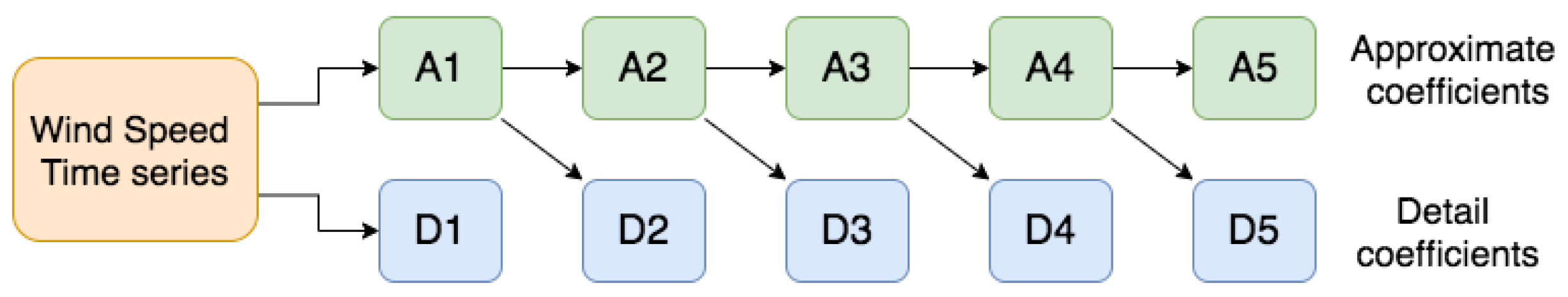
for series length N. This decomposition process is depicted in Figure 1. With an increase in the level of decomposition, more subsignals and specific information about the series over more extended periods emerge. More input features may improve the model’s performance, but they may also lower its computing efficiency and stability. As a result, level-5 decomposition of the wind speed series was used in this investigation [33].
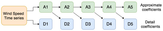
Figure 1.
Wavelet decomposition—level 5.
The WT utilizes the basic wavelet functions identified as mother wavelets. Haar, Daubechies, Biorthogonal, Coiflets, Morlet, and Mexican Hat are some common mother wavelets. To modify the original wind speed time series, we employed the Daubechies (db3) WT with five-level signal decomposition, as previously described.
2.3. Kalman Filter (KF)
A KF is a data processing technique designed to be as efficient as possible. Two steps make up the KF:
- the prediction step
- the correction step
The state is anticipated in the first step using a dynamic mathematical model. It is then corrected with the measurements of the observation model in the second stage, minimizing the estimator’s error covariance [34]. At each step, this cycle continues, with the previous time step’s state serving as the starting value [35]. As a result, the KF is described as a recursive filter that estimates a process via feedback control. Typically, the measured variables supplied to KF facilitate estimation of the state of the process to predict the actual data by taking measurements as input [36,37]. There are different sorts of KF equations: time update and measurement update equations [38,39], given as
The time update equations help project the present state and error covariance estimations to derive an a priori estimate for the next phase. The measurement update equations, on the other hand, provide feedback or add a new measurement to an a priori estimate in order to generate a better posterior estimate [40,41]. The time update equations can be viewed as predictor equations in this context, while the corrector equations can be considered as measurement update equations. Figure 2 shows such a predictor-corrector framework.
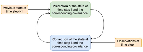
Figure 2.
Flow of Kalman filter.
The keys to successfully applying the KF method are accurately set state, and measurement equations for the KF model initialized using an ARIMA model in this work.
3. Hybrid Models Framework
In this study, we have propose two hybrid methodologies that yield highly accurate short-term wind predictions.
3.1. ARIMA-WT-ML
The wind speed time series is fitted to an ARIMA model, and the residual wind speeds are generated by comparing them to the original data. The following step is to use WT to extract relevant parameters from the wind speed residuals. The approximate and detail coefficients are derived by series decomposition and fed to a supervised ML algorithm—SVR and RF—along with the wind speed time series. We use the MATLAB Wavelet Analysis toolbox for our experiments with the mother wavelet as db3 and level-5 signal decomposition. These WT features are considered independent input features and wind speed as the dependent target variable for the ML model. A 75–25% train-test split precedes the normalization of the training set values with the help of the StandardScaler function in the sklearn python library. Hyperparameter tuning is also conducted in order to fit the ML model, such as SVR, to the best parameters. A list of values for the parameters C, gamma, and kernel has been defined for our experiments. The sklearn library’s GridSearchCV function is used to identify the best potential parameter for the model. For our model implementation, we used a k-fold crossvalidation of ten. The ML method is refitted with these derived best parameter values once the best parameters from the given list have been found. Wind speed is estimated from the unseen test feature set and compared to the actual series test data in the next stage. Finally, the performance is evaluated based on the R2 score, RMSE, and MAE values. This hybrid approach’s step-by-step process is presented in the block diagram shown in Figure 3.
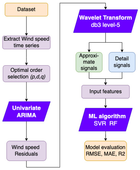
Figure 3.
ARIMA error—WT based hybrid model: ARIMA-WT-SVR/RF.
3.2. KF-WT-ML
Another hybrid approach based on KF is proposed and introduced as a part of our work, and the framework of this method contains three steps. To begin, an ARIMA model aids in the initialization of the state and measurement equations. This process of state initialization through ARIMA makes the KF-WT-ML method an extension or improvement of sorts of the previous method, and the steps of obtaining the state equation in this way are inspired by Liu’s work [16]. We derive the state equation (SE) and measurement equation (ME) before obtaining the wind speed estimation from the KF. Finally, after selecting the right order, we modify the fitted ARIMA model as
As a result, the state equation can be expressed as:
and the measurement equation is formulated as:
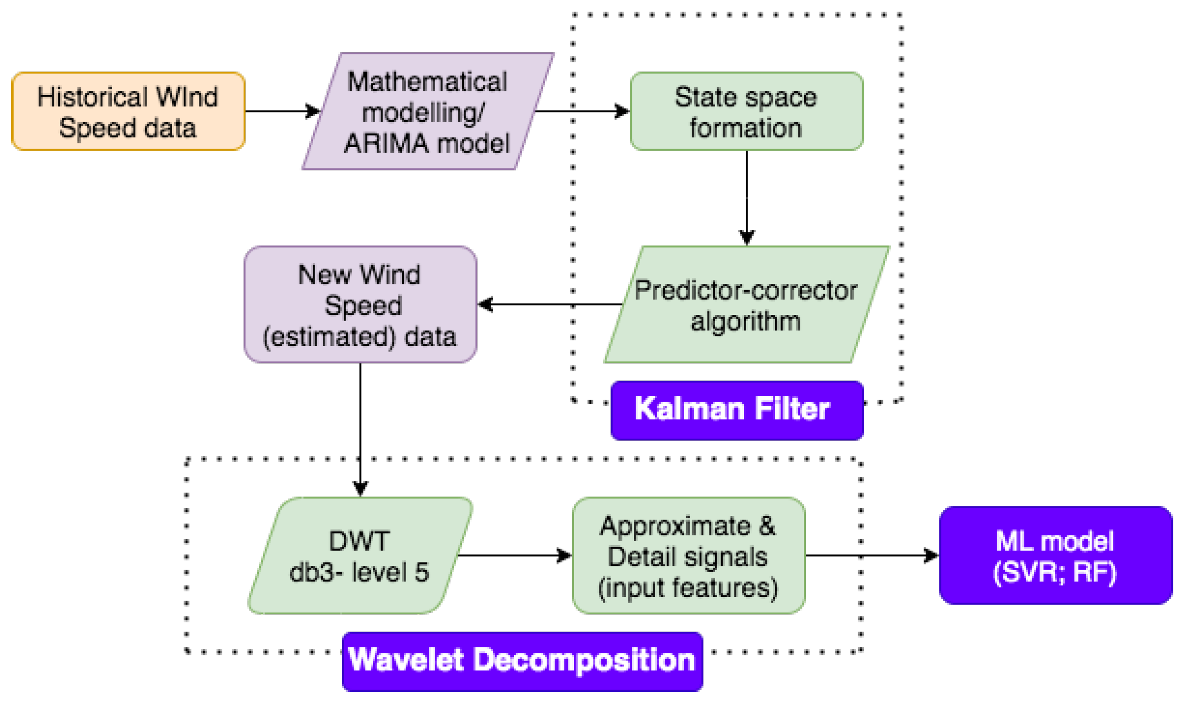
Once initialized, the predictor-corrector KF algorithm is implemented to the SE and ME to estimate the wind speed, using the python library pykalman for the KF process. In the next step, this KF estimated wind speed is fed into the Wavelet Analysis Toolbox (DWT: db3, 5-level) for extracting the best features in the form of approximate and detail signals. Then, with the wind speed as the target variable, the generated approximate, and detail signals are employed as input features to train the ML model. Finally, the model is tested on the 25% test data, and its performance is evaluated based on the evaluation metrics. The block diagram in Figure 4 depicts the model framework of the KF-based hybrid approach.
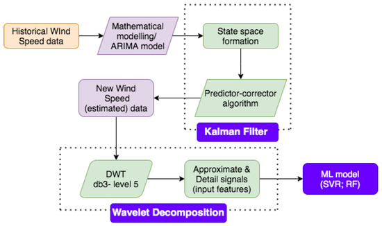
Figure 4.
KF based hybrid model: KF-WT-SVR/RF.
4. Data Description and Evaluation Metrics
To validate the novel approaches introduced, we exposed these models to different sets and data types to determine the outcome and to know their respective potential. Certain evaluation metrics are needed to assess the model’s performance in regression predictions.
4.1. Data Description
To train and test models, we fed data from 10 min, 30 min, and 1 h time interval ranges from various locations around the globe. For a comparison of the proposed models with conventional ML models, we used four different datasets with varied temporal horizons. The 10 min interval TN dataset was taken from Kaggle (www.kaggle.com, accessed on 20 October 2020), while EDP T01 turbine SCADA data was obtained from Energias de Portugal (EDP) open data webpage. In addition, we obtained a 30 min and 1 h time interval dataset from two different geographical locations through a download from the Modern-Era Retrospective analysis for Research and Applications (MERRA) website (www.soda-pro.com/web-services/meteo-data/merra, accessed on 20 October 2020). The detailed description of the datasets implemented in this study is summarized in Table 1. There are four onland datasets in total, with time periods ranging from 10 min to 60 min. In this study, two datasets from the offshore and hilly regions were retrieved and deployed. The average wind speed and standard deviation are also provided in the data description table for each dataset, along with the total number of datapoints.

Table 1.
Datasets and details for short-term forecasting of wind speed.
Offshore wind energy is now seeing a surge in research and development, as these resources are more abundant, powerful, and consistent than land-based wind resources. Therefore, further analysis and comparison across several geographies provide a more in-depth analysis of the KF-based proposed hybrid. In addition, the MERRA website provides wind data for hilly terrain. Finally, the NREL and Orsted public datasets are the source for offshore wind data.
4.2. Evaluation Metrics
The evaluation metrics mentioned below are standard metrics for assessing the model’s performance in regression predictions. The mean absolute error (MAE), root mean square error (RMSE) metrics, and coefficient of determination (R2) help evaluate the presented framework’s performance. In time series analysis, the MAE is a common measure of the forecast error that estimates the average magnitude of the errors. The average of the error between the actual and forecasted data, as represented by MAE, is mathematically given as
where N refers to the number of samples for the total period, is the measured/observed value, and is the estimated/predicted value. As observed, this expression incorporates the error as the absolute error. MAE is less vulnerable to outliers than RMSE because it considers the absolute error. The RMSE is expressed as
The difference between the actual and predicted mean squared error represents values retrieved by squaring the average difference over the data set. The error rate by the square root of MSE is known as RMSE [42]. As depicted by the mathematical equation, RMSE is a quadratic assessment rule to find the average error magnitude. RMSE also gives significant errors disproportionately high weights because errors are squared before being averaged. When substantial errors are avoided, RMSE is most advantageous.
In summary, the model’s performance improves as the RMSE decreases. The coefficient of determination (R2) reflects the goodness of fit compared to the original values, represented as the subtraction of the fraction of the sum of squares of regression and a sum of squares of the total, from unity. The value typically ranges from 0 to 1 and is expressed as a percentage: the greater the value (ideally 1), the more accurate the model:
5. Results and Discussion
Four datasets from various sources, such as EDP energies and the MERRA soda-pro website to cover 10 min, 30 min, and 1 h time intervals of wind data, are utilized in the present study. Comparing the hybrid model results with the state-of-the-art ML methods reveals that the predictions for both the proposed hybrid models have improved significantly.
From Table 2 and Table 3, it is evident that the state-of-the-art ML models perform decently on 10 min interval time-scale datasets. Wind prediction accuracy, on the other hand, could be improved. In terms of R2 score, RMSE, and MAE, the proposed hybrid models produce accurate predictions, indicating that the KF-based hybrid strategy has a modest advantage over the ARIMA-WT-ML model. The R2 scores for both hybrids are over , with the best RMSE of for KF-WT-RF (TN dataset) and for KF-WT-SVR (EDP T01 dataset).
Table 2.
TN [10 min].
Table 3.
EDP T01 [10 min].
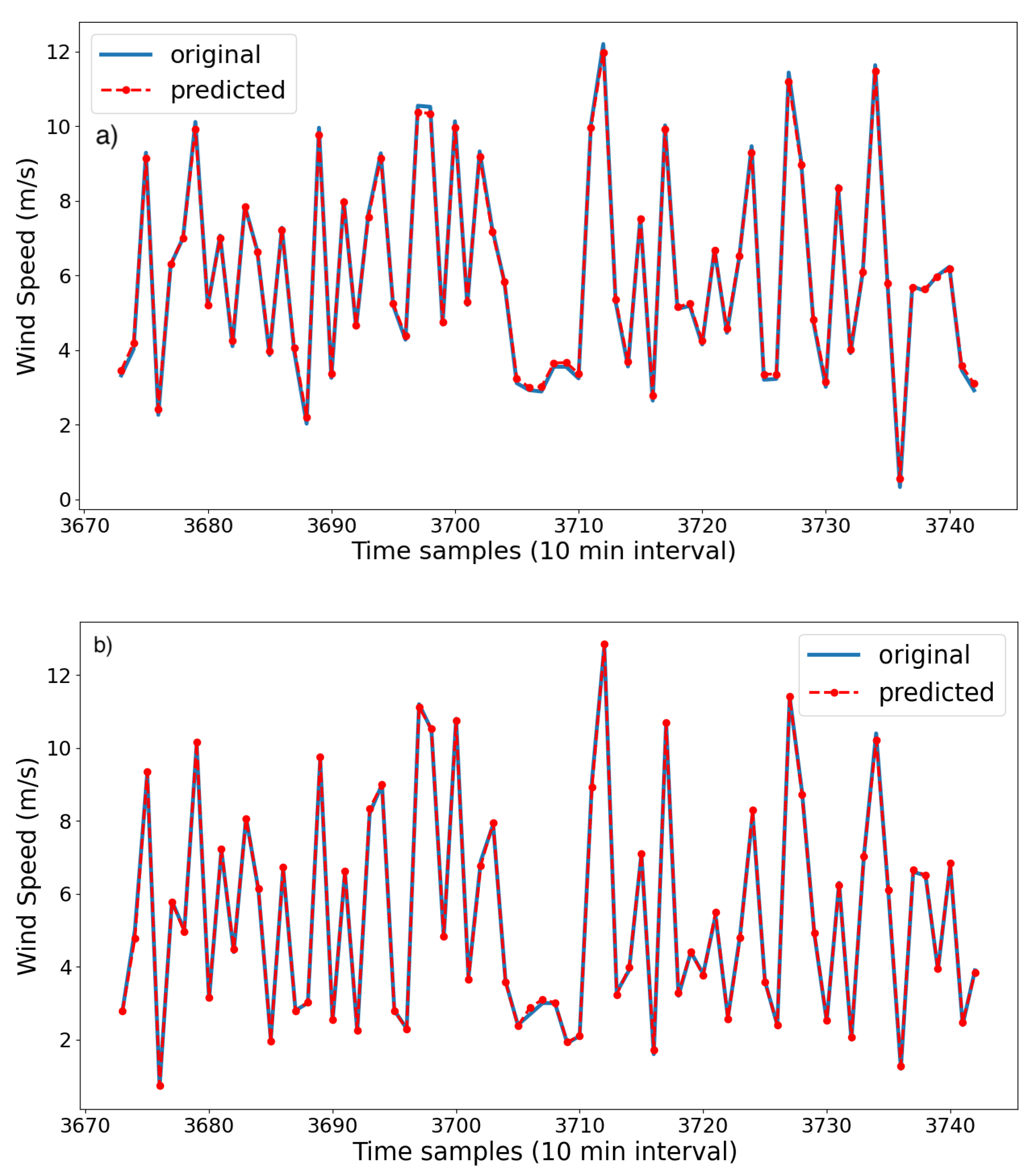
For the TN dataset, there is over a 15% increase in R2 score for the proposed hybrids over the traditional ML models. In addition, this number is about for the EDP T01 dataset. Furthermore, for TN, we observe a significant reduction in error by over for the RMSE evaluator. The case with the error terms of EDP T01 data is similar. In addition, for the data obtained from EDP, the line plots (Figure 5) illustrate the high R2 scores and low root mean and mean absolute errors for both ARIMA-WT and Kalman-WT based techniques. In these time horizons as well, the KF-based hybrid outputs slightly better scores in terms of accuracy and prediction errors.
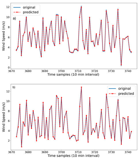
Figure 5.
(a) ARIMA-WT-ML and (b) KF-WT-ML plots for EDP T01 dataset [10 min].
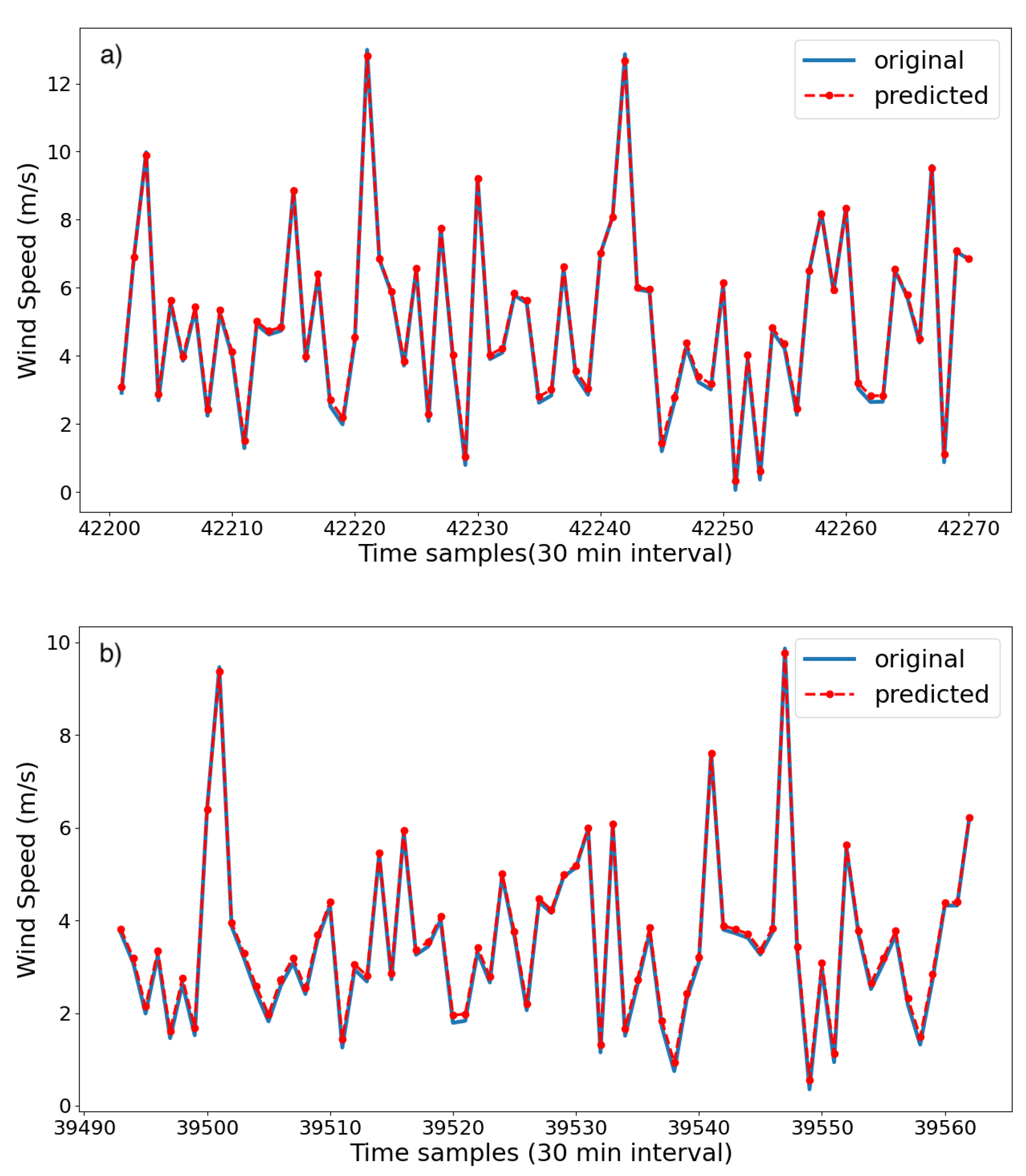
The ML models perform poorly for 30 min and 1 h datasets, as inferred from Table 4 and Table 5. The evaluation metrics show that the R2 scores hover around , and the errors (RMSE and MAE) also range from 1 to 2. However, there is consistency in the proposed hybrid approaches as they perform exceptionally well to give close to precise wind speed forecasts. The R2 scores for both hybrids are over , showing an increment of around 50% for both approaches to provide the best RMSE of 0.01 for KF-WT-RF (30 min) and 0.03 for KF-WT-RF (1 h). In these time horizons, the KF-based hybrid outputs slightly better scores in terms of accuracy and prediction errors. Furthermore, for the dataset collected from MEERA webpage, the line plots, in Figure 6 represent minimal error in terms of predicted and original wind speed data for both the proposed hybrid techniques.
Table 4.
Jaisalmer [30 min].
Table 5.
AWF [1 h].
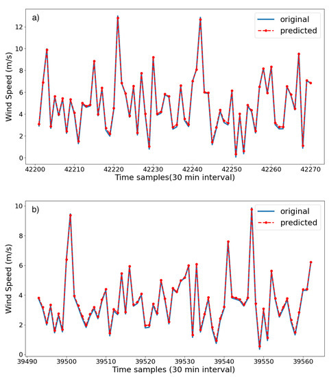
Figure 6.
(a) ARIMA-WT-ML and (b) KF-WT-ML plots for Jaisalmer dataset [30 min].
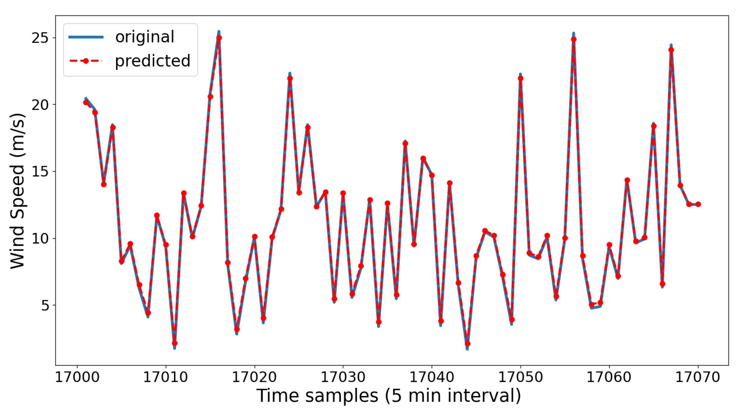
In addition, the KF-based hybrid approach is trained and evaluated on datasets from different terrains and regions around the globe. Along with the onshore, i.e., onland data, a study on two offshore and two hilly region datasets reveals the proposed model’s performance on various terrains. As discussed, the offshore datasets for the Portland coast and the Orsted’s Westermost Rough (WMR) offshore wind farm obtained from NREL Wind Prospector and Orsted webpage, respectively, implement the KF-WL-ML model framework for comparative analysis. Results shown in Table 6 and Table 7 represent a high prediction accuracy from the offshore and hilly regions wind data, as indicated by the R2 score, for all are over the range. However, the errors in the form of RMSE and MAE for the offshore wind speed predictions are relatively larger than onshore wind forecasts. The range of RMSE and MAE for offshore predictions is , while for the onshore forecasts, these errors range between High prediction accuracy wind forecast is obtained for the Kalman-filter-based combination model over different topologies and geographic locations that can be indicated the line plot, in Figure 7, between original and predicted wind speed.
Table 6.
KF-WT-ML(SVR) on different terrains.
Table 7.
KF-WT-ML(RF) on different terrains.
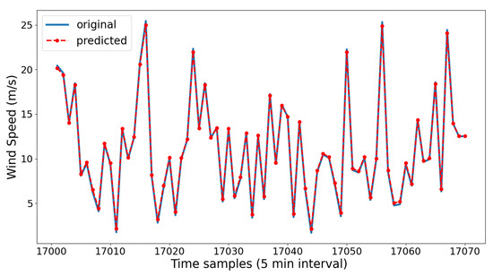
Figure 7.
Offshore NREL KF-WT-ML(SVR).
The model training time is another positive aspect of the proposed hybrids. The models are trained and tested without the requirement of GPU. For almost all the models, the online training time is not more than a few minutes. Training time is in seconds for the datasets with relatively lesser datapoints. The proposed approaches yield more precise wind speed forecasts, as indicated by the statistics of the performance metrics. Furthermore, from the obtained results, the trend of KF based hybrid yielding similar but better scores than that of the ARIMA-WT model is observed over all datasets. One of the reasons for such a trend is the predictor-corrector algorithm which refines the noisy sensor measurements by incorporating a system model and estimates new wind speed series that the WT then processes. The effectiveness of the presented hybrids is demonstrated by the range of datasets implemented, based on various locations, topologies, and time horizons. Furthermore, the consideration of other input features and parameters such as temperature, humidity, and pressure may aid in providing more valuable information about the wind speed, especially for the short-term time horizon.
6. Conclusions
This study investigates short-term forecasting employing two-hybrid approaches that incorporate the ARIMA model, WT, and KF for wind speeds. The hybrid forecasting methods evaluated on four datasets reveal that both the proposed hybrids ARIMA-WT-ML and KF-WT-ML outperform the state-of-the-art ML methods: SVR and RF. Further, the KF based approach is a better regressor for wind speed predictions. On broader time scales, where the conventional ML algorithms failed to give good forecasts, both the hybrid approaches provide significantly precise results with minimal forecast error. Furthermore, when comparing the proposed model’s prediction accuracy across a number of terrains, it was revealed that the proposed model’s prediction accuracy is superior for onshore datasets, followed by offshore wind data. As discussed, it would be interesting to work with newly developed decomposition approaches and ML algorithms in the future, improve the approach for feature selection and more in-depth hyperparameter tuning, and evaluate the predictive accuracy of these models over a long time horizon. Furthermore, deep learning approaches are becoming increasingly popular, and in many applications, they outperform classic machine learning algorithms at the trade-off of longer computer processing times.
Author Contributions
All authors have contributed equally in all the steps of the present work. All authors have read and agreed to the published version of the manuscript.
Funding
This research received no external funding.
Institutional Review Board Statement
Not applicable.
Informed Consent Statement
Not applicable.
Data Availability Statement
The links to the datasets used are included in the manuscript.
Conflicts of Interest
The authors declare no conflict of interest.
References
- Georgilakis, P.S. Technical challenges associated with the integration of wind power into power systems. Renew. Sustain. Energy Rev. 2008, 12, 852–863. [Google Scholar] [CrossRef] [Green Version]
- Smith, J.C.; Milligan, M.R.; DeMeo, E.A.; Parsons, B. Utility wind integration and operating impact state of the art. IEEE Trans. Power Syst. 2007, 22, 900–908. [Google Scholar] [CrossRef]
- Soder, L.; Hofmann, L.; Orths, A.; Holttinen, H.; Wan, Y.; Tuohy, A. Experience from wind integration in some high penetration areas. IEEE Trans. Energy Convers. 2007, 22, 4–12. [Google Scholar] [CrossRef]
- Dhiman, H.S.; Deb, D.; Balas, V.E. Supervised Machine Learning in Wind Forecasting and Ramp Event Prediction; Academic Press: Cambridge, MA, USA, 2020. [Google Scholar]
- Tascikaraoglu, A.; Uzunoglu, M. A review of combined approaches for prediction of short-term wind speed and power. Renew. Sustain. Energy Rev. 2014, 34, 243–254. [Google Scholar] [CrossRef]
- Han, Q.; Meng, F.; Hu, T.; Chu, F. Non-parametric hybrid models for wind speed forecasting. Energy Convers. Manag. 2017, 148, 554–568. [Google Scholar] [CrossRef]
- Chang, W.Y. A literature review of wind forecasting methods. J. Power Energy Eng. 2014, 2, 161. [Google Scholar] [CrossRef]
- Liu, D.; Niu, D.; Wang, H.; Fan, L. Short-term wind speed forecasting using wavelet transform and support vector machines optimized by genetic algorithm. Renew. Energy 2014, 62, 592–597. [Google Scholar] [CrossRef]
- Cadenas, E.; Rivera, W. Wind speed forecasting in three different regions of Mexico, using a hybrid ARIMA–ANN model. Renew. Energy 2010, 35, 2732–2738. [Google Scholar] [CrossRef]
- Liu, H.; Tian, H.Q.; Pan, D.F.; Li, Y.F. Forecasting models for wind speed using wavelet, wavelet packet, time series and Artificial Neural Networks. Appl. Energy 2013, 107, 191–208. [Google Scholar] [CrossRef]
- Xiao, L.; Wang, J.; Dong, Y.; Wu, J. Combined forecasting models for wind energy forecasting: A case study in China. Renew. Sustain. Energy Rev. 2015, 44, 271–288. [Google Scholar] [CrossRef]
- Dhiman, H.S.; Deb, D.; Foley, A.M. Bilateral Gaussian Wake Model Formulation for Wind Farms: A Forecasting based approach. Renew. Sustain. Energy Rev. 2020, 127, 109873. [Google Scholar] [CrossRef]
- Dhiman, H.S.; Anand, P.; Deb, D. Wavelet transform and variants of SVR with application in wind forecasting. In Innovations in Infrastructure; Springer: Singapore, 2019; pp. 501–511. [Google Scholar]
- Bossanyi, E. Short-Term Wind Prediction Using Kalman Filters. Wind. Eng. 1985, 9, 1–8. [Google Scholar]
- Su, Z.; Wang, J.; Lu, H.; Zhao, G. A new hybrid model optimized by an intelligent optimization algorithm for wind speed forecasting. Energy Convers. Manag. 2014, 85, 443–452. [Google Scholar] [CrossRef]
- Liu, H.; Tian, H.-Q.; Li, Y.-F. Comparison of two new ARIMA-ANN and ARIMA-Kalman hybrid methods for wind speed prediction. Appl. Energy 2012, 98, 415–424. [Google Scholar] [CrossRef]
- Hur, S.-H. Short-term wind speed prediction using Extended Kalman filter and machine learning. Energy Rep. 2021, 7, 1046–1054. [Google Scholar] [CrossRef]
- Lio, W.H.; Li, A.; Meng, F. Real-time rotor effective wind speed estimation using Gaussian process regression and Kalman filtering. Renew. Energy 2021, 169, 670–686. [Google Scholar] [CrossRef]
- Zhao, X.; Wei, H.; Li, C.; Zhang, K. A hybrid nonlinear forecasting strategy for short-term wind speed. Energies 2020, 13, 1596. [Google Scholar] [CrossRef] [Green Version]
- Tian, Z.; Chen, H. A novel decomposition-ensemble prediction model for ultra-short-term wind speed. Energy Convers. Manag. 2021, 248, 114775. [Google Scholar] [CrossRef]
- Tian, Z. Modes decomposition forecasting approach for ultra-short-term wind speed. Appl. Soft Comput. 2021, 105, 107303. [Google Scholar] [CrossRef]
- Tian, Z.; Li, H.; Li, F. A combination forecasting model of wind speed based on decomposition. Energy Rep. 2021, 7, 1217–1233. [Google Scholar] [CrossRef]
- Wang, C.; Zhang, S.; Xiao, L.; Fu, T. Wind speed forecasting based on multi-objective grey wolf optimisation algorithm, weighted information criterion, and wind energy conversion system: A case study in Eastern China. Energy Convers. Manag. 2021, 243, 114402. [Google Scholar] [CrossRef]
- Altan, A.; Karasu, S.; Zio, E. A new hybrid model for wind speed forecasting combining long short-term memory neural network, decomposition methods and grey wolf optimizer. Appl. Soft Comput. 2021, 100, 106996. [Google Scholar] [CrossRef]
- Duan, J.; Zuo, H.; Bai, Y.; Duan, J.; Chang, M.; Chen, B. Short-term wind speed forecasting using recurrent neural networks with error correction. Energy 2021, 217, 119397. [Google Scholar] [CrossRef]
- Karasu, S.; Saraç, Z. Classification of power quality disturbances by 2D-Riesz Transform, multi-objective grey wolf optimizer and machine learning methods. Digit. Signal Process. 2020, 101, 102711. [Google Scholar] [CrossRef]
- Martinez-García, F.P.; Contreras-de Villar, A.; Muñoz-Perez, J.J. Review of Wind Models at a Local Scale: Advantages and Disadvantages. J. Mar. Sci. Eng. 2021, 9, 318. [Google Scholar] [CrossRef]
- Singh, S.; Mohapatra, A. Repeated wavelet transform based ARIMA model for very short-term wind speed forecasting. Renew. Energy 2019, 136, 758–768. [Google Scholar]
- Dhiman, H.S.; Deb, D. Machine intelligent and deep learning techniques for large training data in short-term wind speed and ramp event forecasting. Int. Trans. Electr. Energy Syst. 2021, 31, e12818. [Google Scholar] [CrossRef]
- Bajric, R.; Zuber, N.; Skrimpas, G.A.; Mijatovic, N. Feature extraction using discrete wavelet transform for gear fault diagnosis of wind turbine gearbox. Shock Vib. 2016, 2016, 6748469. [Google Scholar] [CrossRef] [Green Version]
- Catalão, J.P.d.S.; Pousinho, H.M.I.; Mendes, V.M.F. Short-term wind power forecasting in Portugal by neural networks and wavelet transform. Renew. Energy 2011, 36, 1245–1251. [Google Scholar] [CrossRef]
- Dhiman, H.S.; Deb, D.; Guerrero, J.M. Hybrid machine intelligent SVR variants for wind forecasting and ramp events. Renew. Sustain. Energy Rev. 2019, 108, 369–379. [Google Scholar] [CrossRef]
- Yang, M.; Sang, Y.F.; Liu, C.; Wang, Z. Discussion on the choice of decomposition level for wavelet based hydrological time series modeling. Water 2016, 8, 197. [Google Scholar] [CrossRef] [Green Version]
- Haney, S.A. High Content Screening: Science, Techniques and Applications; John Wiley & Sons: Hoboken, NJ, USA, 2008. [Google Scholar]
- Romanna, S.; Lingras, P.; Sombattheera, C.; Krishna, A. Multi-Disciplinary Trends in Artificial Intelligence: 7th International Workshop, MIWAI 2013, Krabi, Thailand, December 9–11. 2013, Proceedings; Springer: Berlin/Heidelberg, Germany, 2013; Volume 8271. [Google Scholar]
- Kleinbauer, R. Kalman Filtering Implementation with Matlab; University of Stuttgart: Stuttgar, Germany, 2004. [Google Scholar]
- Gupta, S.; Singh, A.P.; Deb, D.; Ozana, S. Kalman Filter and Variants for Estimation in 2DOF Serial Flexible Link and Joint Using Fractional Order PID Controller. Appl. Sci. 2021, 11, 6693. [Google Scholar] [CrossRef]
- Louka, P.; Galanis, G.; Siebert, N.; Kariniotakis, G.; Katsafados, P.; Pytharoulis, I.; Kallos, G. Improvements in wind speed forecasts for wind power prediction purposes using Kalman filtering. J. Wind. Eng. Ind. Aerodyn. 2008, 96, 2348–2362. [Google Scholar] [CrossRef] [Green Version]
- Khoshrodi, M.N.; Jannati, M.; Sutikno, T. A Review of Wind Speed Estimation for Wind Turbine Systems Based on Kalman Filter Technique. Int. J. Electr. Comput. Eng. 2016, 6, 1406. [Google Scholar]
- Welch, G.; Bishop, G. An Introduction to the Kalman Filter; Department of Computer Science, University of North Carolina at Chapel Hill: Chapel Hill, NC, USA, 17 December 1997. [Google Scholar]
- Abdelgawad, A.M. Resourse-Aware Data Fusion Algorithms for Wireless Sensor Networks. Ph.D. Thesis, University of Louisiana at Lafayette, Lafayette, LA, USA, 2011. [Google Scholar]
- Kassambara, A. Machine Learning Essentials: Practical Guide in R. 2018. Available online: http://www.sthda.com (accessed on 20 October 2020).


Publisher’s Note: MDPI stays neutral with regard to jurisdictional claims in published maps and institutional affiliations. |
© 2022 by the authors. Licensee MDPI, Basel, Switzerland. This article is an open access article distributed under the terms and conditions of the Creative Commons Attribution (CC BY) license (https://creativecommons.org/licenses/by/4.0/).