Proceeding Paper

Magnetohydrodynamic Equilibrium Reconstruction with Consistent Uncertainties †

by
Robert Köberl
1,2,*,
Robert Babin
1,3 and
Christopher G. Albert
3
1
Max-Planck-Institute for Plasma Physics, 85748 Garching, Germany
2
School of Computation, Information and Technology (CIT), Technical University of Munich (TUM), 85748 Garching, Germany
3
Fusion@ÖAW, Institut für Theoretische Physik Computational Physics (ITPcp), Technische Universität Graz (TU Graz), 8010 Graz, Austria
*
Author to whom correspondence should be addressed.
Presented at the 42nd International Workshop on Bayesian Inference and Maximum Entropy Methods in Science and Engineering, Garching, Germany, 3–7 July 2023.
Phys. Sci. Forum 2023, 9(1), 6; https://doi.org/10.3390/psf2023009006
Published: 27 November 2023

Abstract

:
We report on progress towards a probabilistic framework for consistent uncertainty quantification and propagation in the analysis and numerical modeling of physics in magnetically confined plasmas in the stellarator configuration. A frequent starting point in this process is the calculation of a magnetohydrodynamic equilibrium from plasma profiles. Profiles, and thus the equilibrium, are typically reconstructed from experimental data. What sets equilibrium reconstruction apart from usual inverse problems is that profiles are given as functions over a magnetic flux derived from the magnetic field, rather than spatial coordinates. This makes it a fixed-point problem that is traditionally left inconsistent or solved iteratively in a least-squares sense. The aim here is progressing towards a straightforward and transparent process to quantify and propagate uncertainties and their correlations for function-valued fields and profiles in this setting. We propose a framework that utilizes a low-dimensional prior distribution of equilibria, constructed with principal component analysis. A surrogate of the forward model is trained to enable faster sampling.

1. Introduction

A frequent starting point for calculations in magnetic confinement fusion is the magnetohydrodynamic equilibrium. Ideal magnetohydrodynamics (MHD) [1] describes plasma as a single quasi-neutral fluid under the assumptions of infinite electrical conductivity, small ion gyroradius and negligible electron momentum. An MHD equilibrium is a solution to the static MHD equations (Equations (1)–(3)), describing the magnetic field ( B ) and its relation to the current density ( J ) and the pressure (p):
J × B = p ,
× B = μ 0 J ,
· B = 0 .
The solutions to Equations (1)–(3) are typically obtained in magnetic flux coordinates [2], curvilinear coordinates that greatly simplify calculations, for example, by aligning in such a way that B appears straight. A large part of a typical MHD solution is, therefore, the mapping from flux coordinates to real-space coordinates. Inferring an MHD equilibrium from experimental diagnostics, a task known as equilibrium reconstruction, is of great interest for fusion experiments, to gain insight into unmeasurable or hard-to-measure quantities [3], such as flux surface geometry.
This task is routinely performed for tokamaks [4,5], where the toroidal symmetry further simplifies the MHD equations but proves to be more complicated for three dimensional (3D) systems, like stellarators. Typically, MHD solvers take the pressure and toroidal current profile as functions of a radial flux coordinate ρ as input and solve for the optimal geometry of the magnetic flux surfaces. From the resulting equilibrium configuration, synthetic diagnostic signals can be calculated and compared to the corresponding real physical measurements. This makes 3D equilibrium reconstruction a fixed-point problem that is traditionally solved iteratively in a least-squares sense [3,6,7]. While the least-squares approach can result in suitable reconstructed parameters and uncertainty estimates [8], evaluations of the forward model are computationally demanding (a single equilibrium reconstruction can take up to several hours [9,10]), and common error estimates might fail to capture relevant uncertainties when high levels of noise are present for the equilibrium diagnostics [11]. Existing Bayesian frameworks [12] are also limited by the high computational costs of the forward model. Therefore, we aim to build a Bayesian framework for 3D equilibrium reconstruction that allows for fast sampling from the posterior distribution of equilibria while maintaining relevant physical constraints. In this work, we present, as a proof of concept, such a framework for a configuration of the Wendelstein 7-X stellarator (W7-X).

2. Methods

For the proposed equilibrium reconstruction approach using the Bayesian formalism, two major components are required: a prior distribution of equilibria and a fast evaluation of the likelihood function, both of which are not readily accessible. A schematic depiction of the steps taken to obtain these major components is shown in Scheme 1. To define the prior distribution of equilibria, a physically motivated prior distribution over equilibrium-defining parameters is formulated (Section 2.1). Samples from this prior distribution are then propagated into the space of equilibria using the Variational Moments Equilibrium Code (VMEC) [13] (Section 2.2) and subsequently into the space of synthetic equilibrium diagnostic signals with the code DIAGNO [14]. Since the space of equilibria is very high-dimensional, dimensionality reduction is performed on the equilibria using principal component analysis (PCA) (Section 2.3). In this way, a low-dimensional distribution over equilibrium configurations, which enables the training of polynomial chaos expansion (PCE) [15] surrogate models, can be defined (Section 2.4). These models map low-dimensional parameters c i onto the space of synthetic equilibrium diagnostic signals and thus circumvent high computational costs arising from the DIAGNO forward model. Through the combination of the surrogates with the low-dimensional equilibrium prior, the low-dimensional posterior distribution of equilibrium parameters can be inferred using Markov Chain Monte Carlo (MCMC) sampling in a Bayesian formalism, based on a set of (synthetic) measurement signals (Section 3).

2.1. Prior Distribution of Current and Pressure Profiles

We define a prior distribution for pressure p s and toroidal current I s profiles. They are functions of normalized toroidal flux s = ψ ψ 0 and define an MHD equilibrium together with the total toroidal flux ( ψ 0 ). Here, ψ denotes the toroidal flux. Often, reconstruction methods utilize simple parameterized functions [3,7,8], for example, two-power profiles, for describing equilibrium profiles. In order not to restrict the method to only favorable profiles, a broader prior is desired. Following similar concepts already realized in the MINERVA framework [10,12,16], we propose the use of a Gaussian Process [17] (GP) as a function generator for the profile gradients. This allows us to more easily specify the length scales and smoothness constraints based on physics information. For the pressure profile, the correlation length scales are larger at the core of the plasma than at the boundary, which is encoded in the GP kernel used in the MINERVA framework for W7-X [10]. We further constrain the pressure profile to be monotonic and 0 at the plasma boundary and enforce these constraints with exponentiation and integration, as well as a renormalization. For the current profile GP, a smooth rational quadratic kernel [17] is used, since detailed information on the current profile shape can be hard to capture with magnetic diagnostics alone [11] and the toroidal current is expected to be comparatively low for standard W7-X equilibria. Again, exponentiation and integration ensure monotonicity, but in contrast to the pressure profile, the current is 0 at the magnetic axis, and the scaling factor can be positive or negative. Using exponentiation as a positivity transform for the profile gradients allows for steep gradients but discourages many local plateaus that are found when using the absolute value as the transform.
p ˜ s G P Minerva                                 p s = p 0 0 1 exp p ˜ d s s 1 exp p ˜ d s
I ˜ s G P RQ                                           I s = I 0 0 1 exp I ˜ d s 1 s exp I ˜ d s
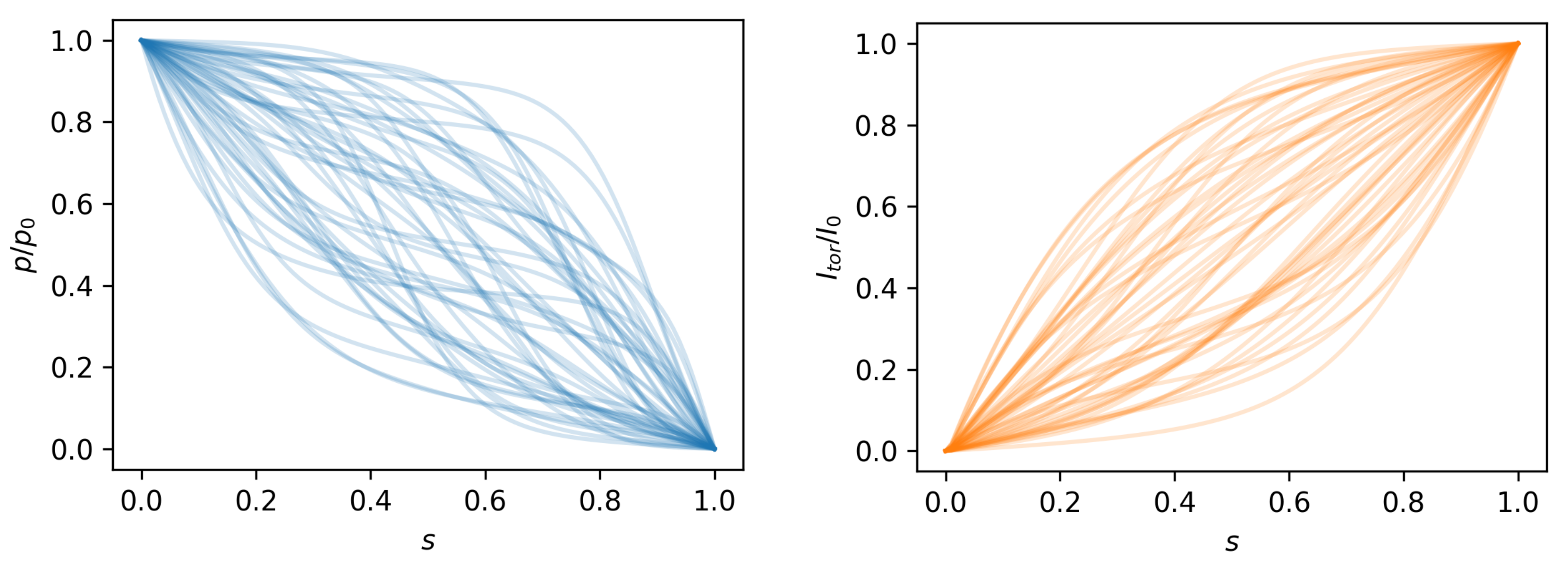
Finally, the GP is approximated with a PCA to allow for the space-filling latin hypercube sampling of the parameter space. Six shape parameters for the pressure profile and three shape parameters for the current profile correspond to an explained variance ratio of 99 % each. Combined with a parameter ψ 0 for the total toroidal magnetic flux, this gives us 12 equilibrium-defining parameters, as detailed in Table 1. Several realizations of the equilibrium profile shapes obtained with the described procedure are visualized in Figure 1. From the prior defined in Table 1, 4000 samples are drawn and propagated into the space of MHD equilibria using VMEC.

2.2. VMEC

VMEC solves Equations (1)–(3) using a double-Fourier basis for the inverse coordinate representation x ρ , θ , ζ = R , Z , ϕ . Here, ρ = s denotes the magnetic flux surfaces, and θ and ζ are poloidal and toroidal angle-like flux coordinates. VMEC uses an energy functional in place of the local formulation, which is guaranteed to converge to an equilibrium in the absence of magnetic islands. This is not guaranteed for 3D geometries like stellarators [2], but VMEC can provide a suitable approximation of magnetic flux surfaces. In contrast to many other equilibrium codes, VMEC does not require a fixed plasma boundary but can calculate equilibrium flux surfaces, including the last closed flux surface, given a coil current configuration i 1 . . . i 5 , as well as ψ 0 , p s and I s .
A VMEC equilibrium can be fully described by the Fourier series for cylindrical coordinates R ρ , θ , ζ , Z ρ , θ , ζ and potential λ ρ , θ , ζ , rotational transform profile ι ρ = d χ d ψ and total toroidal flux ψ 0 = ψ ρ = 1 . Here, χ denotes the poloidal flux, and the cylindrical angle ( ϕ ) is a periodic continuation of the toroidal angle ( ζ ) with the number of field periods ( N F P ). The straight-field-line angle ( θ = θ + λ ρ , ζ , θ ) can be calculated from λ . With stellarator symmetry, the Fourier series for R only contains cosine components, while Z and λ only contain sine components. For the radial direction, VMEC uses a finite difference scheme and a linear spacing in the normalized toroidal flux s = ρ 2 = ψ ψ 0 .
The pressure profile ( p ρ ) can be calculated with a weak formulation of the radial force balance [13] under the assumption that Equation (1) is fulfilled:
p ρ = ρ 1 1 μ 0 J d ψ d ρ d d ρ B ζ + ι d d ρ B θ d ρ
where Q = 1 4 π 2 Q d θ d ζ denotes an average over a flux surface and J is the determinant of the Jacobian.

2.3. Dimensionality Reduction

With S = 99 radial points, M = 25 poloidal modes and N = 12 toroidal modes, a VMEC equilibrium can be described using S · M · N parameters for R, Z and λ , respectively; S parameters for ι ; and a single parameter for ψ 0 . With a total of 85,636 non-zero parameters, this space is difficult to handle with Bayesian methods. To reduce the dimensionality, principal component analysis (PCA) was applied on the VMEC equilibria.
To compensate for the incomparable units of the five quantities, they were all rescaled such that the total variance of each group of parameters was 1. For the total explained variance ratio of 99.9 % , it was found that 11 principal components were sufficient to represent the equilibrium prior. The comparatively low dimensionality now facilitates Bayesian inference directly on the equilibrium parameters and also significantly reduces the number of data needed to represent the posterior distribution or a collection of samples.
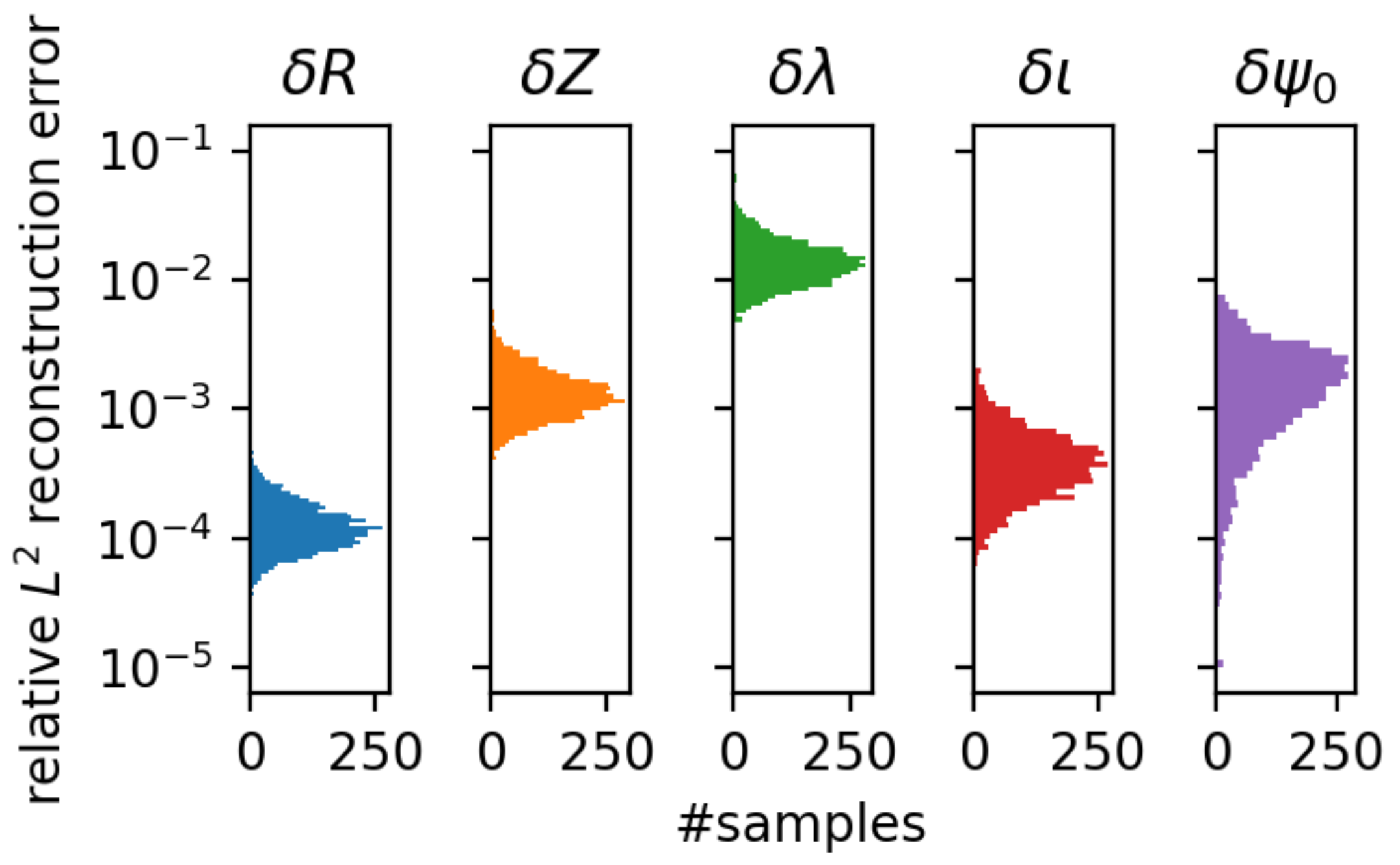
For each of the five quantities R , Z , λ , ι and ψ 0 , the reconstruction error due to dimensionality reduction was evaluated using the L 2 metric (Figure 2). The relative error stayed below 1 % for all quantities except λ . This lead to lower quality of the direction of B and derived quantities like p. The distribution of the low-dimensional parameters ( c i ) was approximated with kernel density estimation (KDE) and assumed to be independent. This assumption held well enough and marginally increased the width of the total prior.
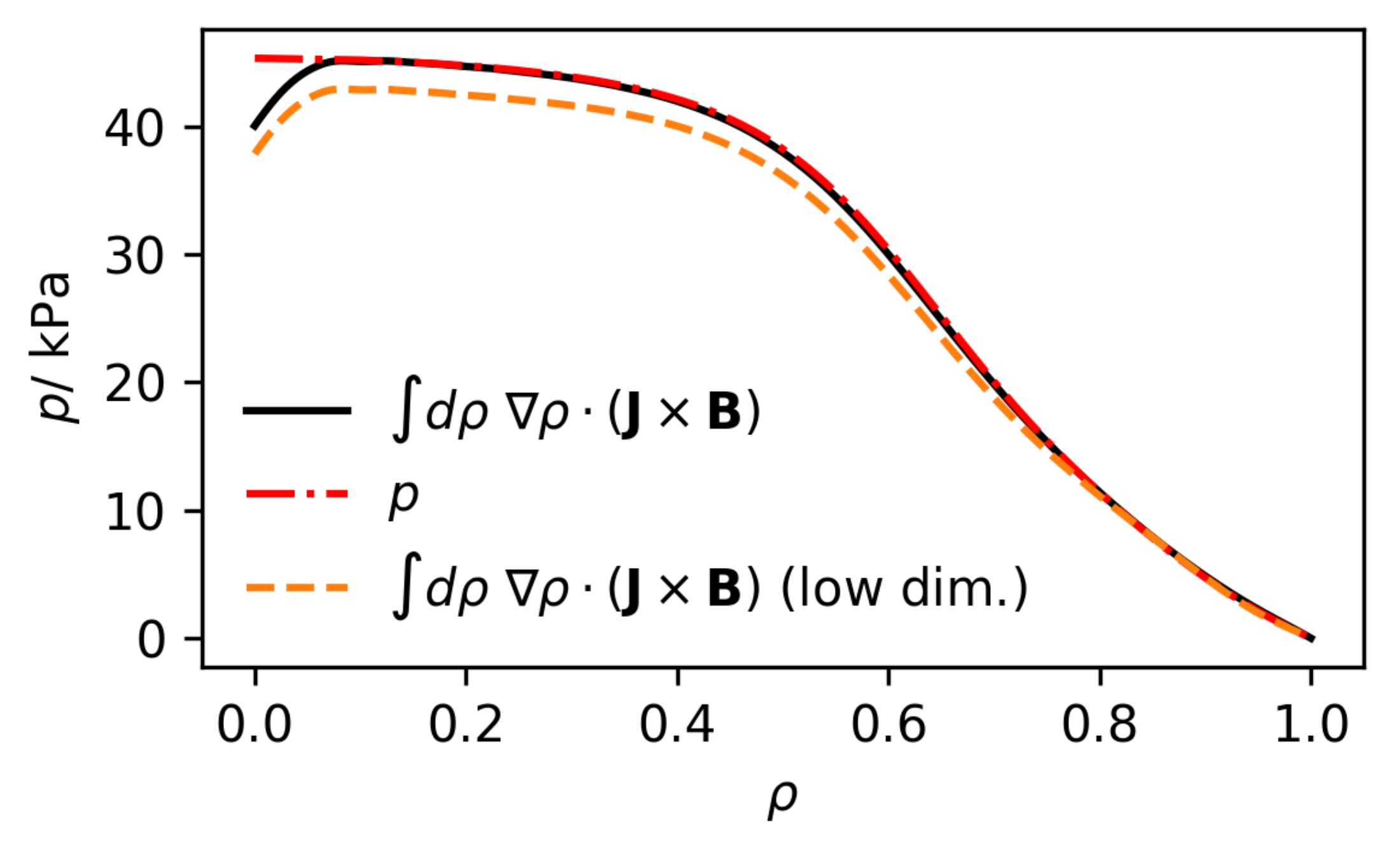
In Figure 3, the pressure profile is shown for a validation sample drawn from the prior distribution, together with a pressure profile calculated with Equation (6), and the same calculation applied after the validation sample was pushed through the dimensionality reduction. Indeed, the pressure profile can be calculated from the five quantities R , Z , λ , ι and ψ 0 , which determine J and B , with only a small deviation near the magnetic axis, where VMEC is known to be inaccurate. However, dimensionality reduction significantly reduces the accuracy of this calculation.

2.4. Synthetic Diagnostics Surrogate Model

We trained polynomial chaos expansion (PCE) surrogate models that map from equilibrium coefficients c i to magnetic equilibrium diagnostics of W7-X. The aim of these surrogate models was to circumvent prohibitively high computational costs arising from DIAGNO forward model evaluations, which occur during sampling. The magnetic equilibrium diagnostics considered were saddle coils, diamagnetic loops and segmented Rogowski coils [18]. PCEs were built using the linear regression methods provided in the chaospy [19] Python package. The polynomials used in the expansions were chosen through hyperbolic truncation. In this truncation scheme, all multivariate polynomials, where the associated degrees of the univariate polynomials α i fulfill [20]
d i α i h 1 / h ,
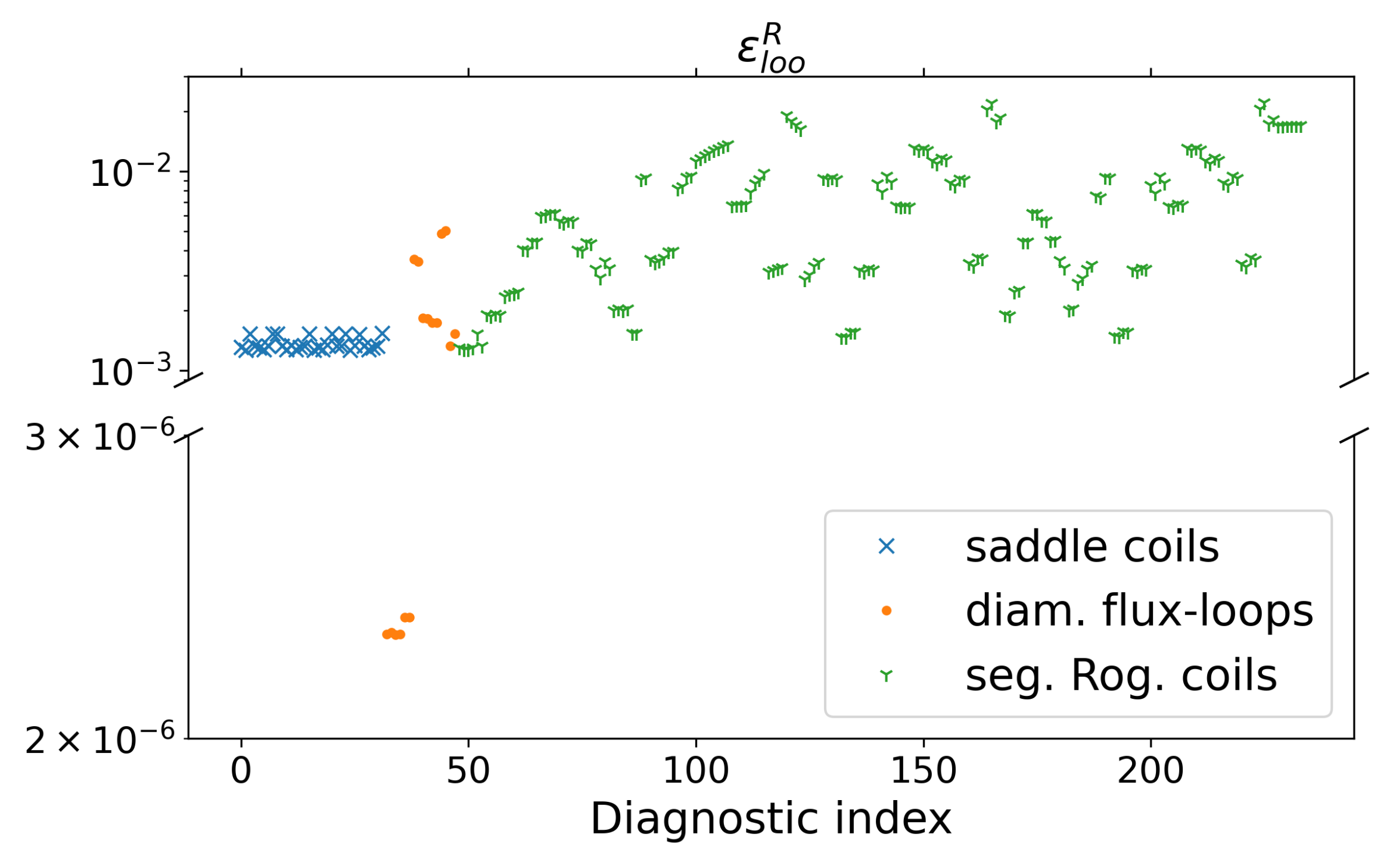
are retained. Here, d denotes the maximum polynomial degree occurring in the expansion, and h ( 0 , 1 ] determines the number of retained polynomials. While several other methods for choosing the basis polynomials in a sparse sense exist [21], we found that the hyperbolic truncation scheme with d = 6 and h = 0.8 worked well in the considered case. To estimate the performance of the resulting PCEs, the relative leave-one-out error ε l o o R [22] was calculated for each surrogate model. The resulting ε l o o R for these PCEs are visualized in Figure 4, grouped in terms of the synthetic diagnostic signal that is being approximated. Note that ε l o o R is given relative to the variance present in the training data.

3. Results

With the previously discussed prior on the low-dimensional parameters ( c i ) and the synthetic diagnostic surrogate, we tried to reconstruct a W7-X standard configuration equilibrium from a set of corresponding synthetic magnetic equilibrium diagnostic signals.
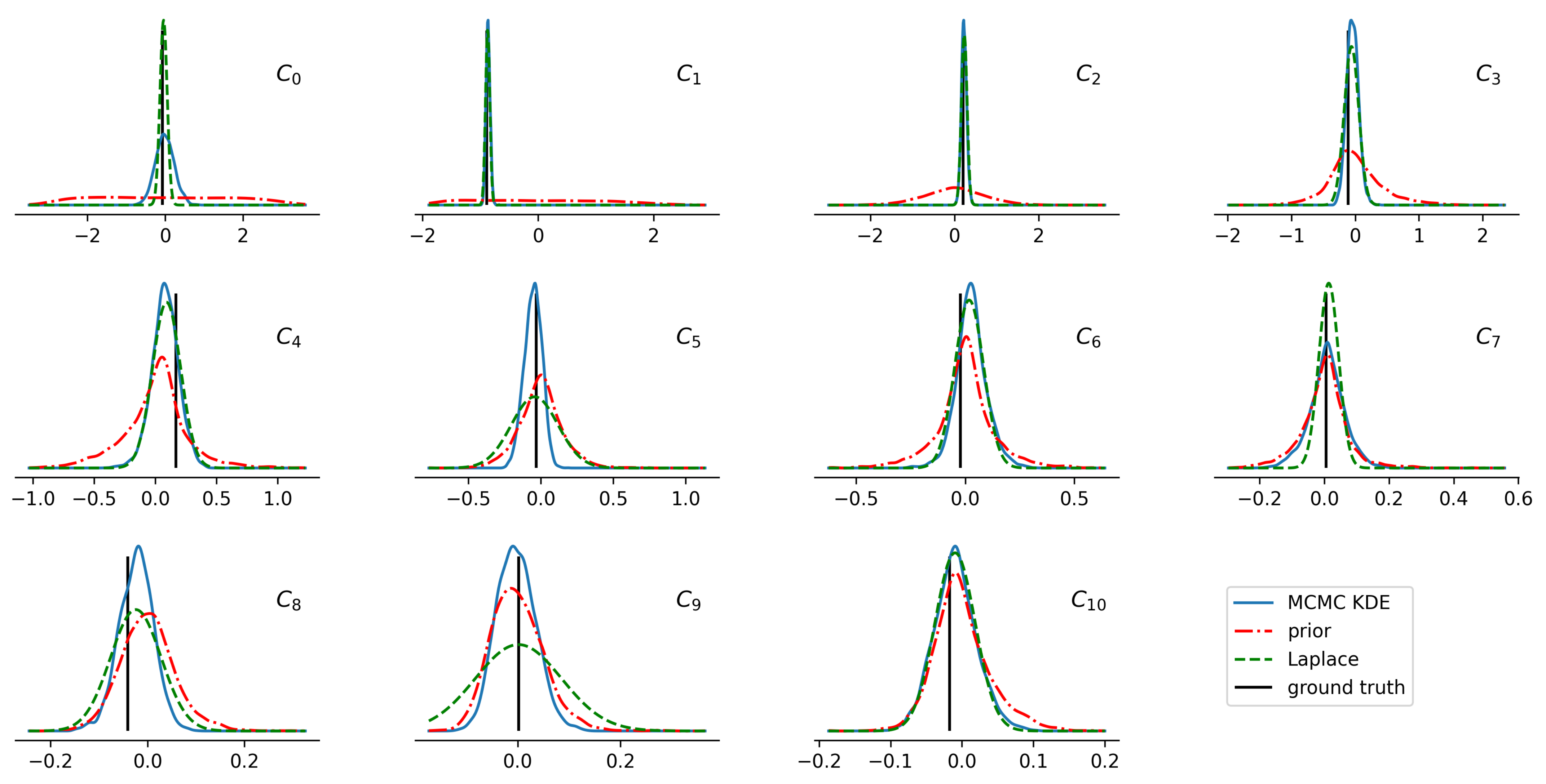
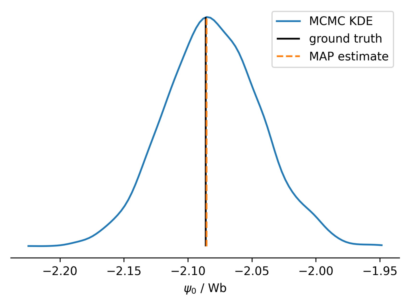
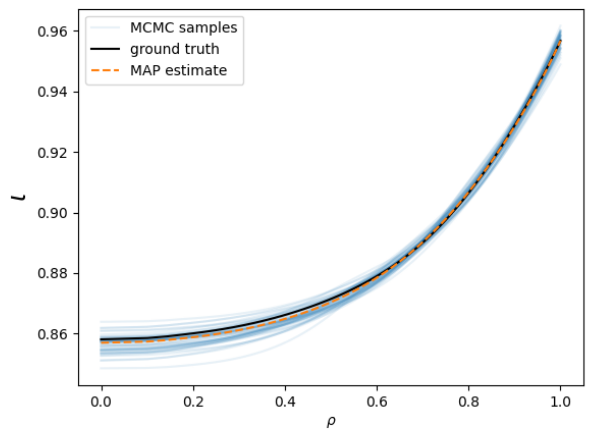
A set of equilibrium-defining parameters from the distribution discussed in Section 2.1 were propagated using the VMEC/DIAGNO forward model, providing a known ground truth. The resulting synthetic magnetic equilibrium diagnostic signals were then used together with a Gaussian likelihood function and the low-dimensional equilibrium prior to estimate the posterior distribution of c i . For the likelihood function, the synthetic diagnostics were assumed to be uncorrelated with a 5 % error. Two methods for estimating the posterior were used: Laplace’s approximation and MCMC sampling. In both methods the evaluation of the synthetic magnetic equilibrium diagnostics was performed with the PCE surrogate models. For the MCMC method, samples were drawn using NUTS [23]. Figure 5 depicts one-dimensional projections of the posterior estimates for the parameters c i with respect to the associated prior distribution. Seen with respect to the prior width, there is a high uncertainty in the posterior distribution of parameters c 4 to c 10 . However, they contribute little to the explained variance of the equilibrium PCA. To visualize how this estimated uncertainty appears in the physically relevant space, the maximum a posteriori estimate (MAP) and several samples were transformed back into the space of VMEC equilibria. The flux surface geometry, total toroidal flux and rotational transform profile are visualized in Figure 6, Figure 7 and Figure 8, respectively. In addition to the reconstructed equilibria, the ground-truth evaluation of VMEC is visualized. One can observe that the MAP estimate is comparatively close to the ground-truth values and that for all three quantities, the ground-truth value is covered within the area spanned by the posterior samples.
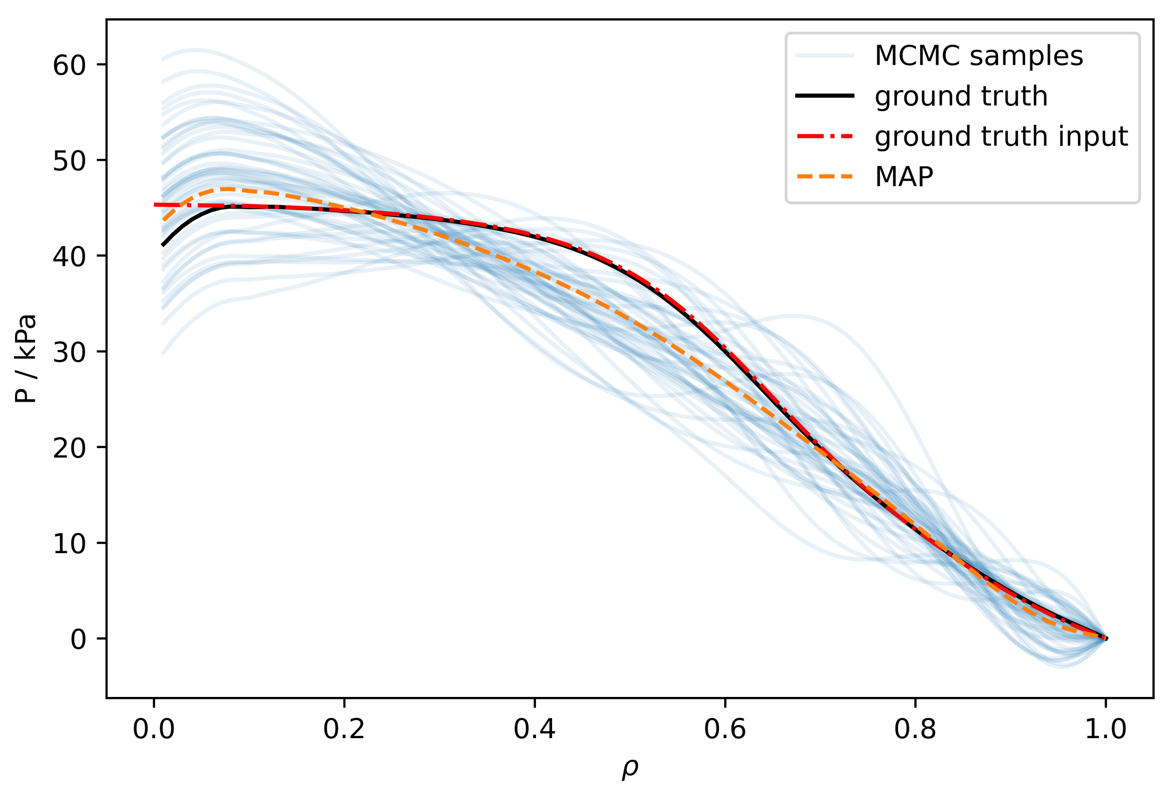
With Equation (6), the radial pressure profile of the posterior samples can be estimated (Figure 9). Significant differences between the MAP estimate and the ground-truth profile can be observed. However, the ground-truth profile is still covered within the space spanned by the posterior samples, and the magnetic diagnostics used for this reconstruction are rather insensitive to the pressure profile. The systematic discrepancy close to the magnetic axis can be attributed to the use of VMEC, which is known to have problems in this region. Additionally, the profile shapes expose nonphysical values near the last closed flux surface, as well as non-monotonicity, which was not present in the pressure profile prior. One reason for this, as shown above in Figure 3, is that PCA dimensionality reduction affects the derived pressure profile more than magnetic quantities, like the rotational transform profile (Figure 2).

4. Discussion

The results presented in Section 3 show that the presented framework is able to reconstruct an equilibrium configuration drawn from the prior distribution. That is, the ground truth lies within the region of high probability of the estimated posterior distributions, and the MAP estimate closely matches the true flux surface geometry and rotational transform profile. While the MAP estimate and posterior mean are found to be equivalent, Laplace’s approximation is not sufficient to model the posterior. Quantities that are derived from the magnetic quantities R , Z , λ , ι and ψ 0 , such as pressure profile p J , B are not reconstructed well, partially due to dimensionality reduction, but also because the considered magnetic diagnostics are not very sensitive to the pressure profile. While the derived pressure profiles fulfill the weak force balance by construction, they lack the physically motivated constraints that are encoded into the profile prior distribution in Section 2.1. In particular, they can violate the positivity constraint. However, the true profile does lie within the posterior distribution, and a pressure-sensitive diagnostic could be used to determine it, particularly as the mapping between real-space and flux coordinates is reconstructed well.
The presented framework offers a flexible prior distribution of profiles but directly reconstructs the flux surface geometry from magnetic diagnostics, allowing samples of the flux surface geometry to be drawn from the posterior. The equilibrium prior has to be constructed once for each device configuration, e.g., coil currents, but it offers reusability from this point onward and can be well described with only a few principal components. This not only allows Bayesian methods to be applied effectively but also significantly reduces the number of data needed to describe a posterior distribution or collection of samples. The PCE surrogate model similarly reduces the computational cost of 3D equilibrium reconstruction and offers fast access to uncertainties.
With the presented methods, we provide a proof of concept for a fast Bayesian equilibrium reconstruction framework. The accurate reconstruction of the derived quantities and thus the physical consistency of the posterior samples warrant further investigation. This could be achieved with different dimensionality reduction methods, for example, using a variational autoencoder with additional physics constraints, or different surrogate models, as well as more accurate MHD solvers.

Author Contributions

Conceptualization, R.K., R.B. and C.G.A.; methodology, R.K., R.B. and C.G.A.; software, R.K. and R.B.; investigation, R.K. and R.B.; data curation, R.K. and R.B.; writing—original draft preparation, R.K. and R.B.; writing—review and editing, R.K., R.B. and C.G.A.; visualization, R.K. and R.B.; supervision, R.K. and C.G.A.; project administration, C.G.A.; funding acquisition, C.G.A. All authors have read and agreed to the published version of the manuscript.

Funding

The present contribution was supported by the Helmholtz Association of German Research Centers under the joint research school HIDSS-0006 ’Munich School for Data Science - MUDS’. This work was carried out within the framework of the EUROfusion Consortium, funded by the European Union via the Euratom Research and Training Programme (Grant Agreement No. 101052200-EUROfusion). Views and opinions expressed are, however, those of the authors only and do not necessarily reflect those of the European Union or the European Commission. Neither the European Union nor the European Commission can be held responsible for them.

Institutional Review Board Statement

Not applicable.

Informed Consent Statement

Not applicable.

Data Availability Statement

The data presented in this study are openly available via Zenodo at https://doi.org/10.5281/zenodo.8063360 (accessed on 21 June 2023).

Acknowledgments

The authors thank Udo von Toussaint, Florian Hindenlang and Omar Maj for insightful discussions, and the reviewers for their helpful remarks.

Conflicts of Interest

The authors declare no conflict of interest.

References

  1. Freidberg, J.P. Ideal MHD; Cambridge University Press: New York, NY, USA, 2014. [Google Scholar]
  2. D’haeseleer, W.D.; Hitchon, W.N.G.; Callen, J.D.; Shohet, J.L. Flux Coordinates and Magnetic Field Structure; Springer: Berlin/Heidelberg, Germany, 1991. [Google Scholar] [CrossRef]
  3. Lazerson, S.; The DIII-D Team. Three-Dimensional Equilibrium Reconstruction on the DIII-D Device. Nucl. Fusion 2015, 55, 023009. [Google Scholar] [CrossRef]
  4. Fischer, R.; Fuchs, C.J.; Kurzan, B.; Suttrop, W.; Wolfrum, E.; ASDEX Upgrade Team. Integrated Data Analysis of Profile Diagnostics at ASDEX Upgrade. Fusion Sci. Technol. 2010, 58, 675–684. [Google Scholar] [CrossRef]
  5. Fischer, R.; Giannone, L.; Illerhaus, J.; McCarthy, P.J.; McDermott, R.M.; ASDEX Upgrade Team. Estimation and Uncertainties of Profiles and Equilibria for Fusion Modeling Codes. Fusion Sci. Technol. 2020, 76, 879–893. [Google Scholar] [CrossRef]
  6. Andreeva, T.; Alonso, J.; Bozhenkov, S.; Brandt, C.; Endler, M.; Fuchert, G.; Geiger, J.; Grahl, M.; Klinger, T.; Krychowiak, M.; et al. Equilibrium Evaluation for Wendelstein 7-X Experiment Programs in the First Divertor Phase. Fusion Eng. Des. 2019, 146, 299–302. [Google Scholar] [CrossRef]
  7. Sanders, M.; Ida, K.; Yoshinuma, M.; Suzuki, C.; Yoshimura, Y.; Seki, R.; Emoto, M.; Yoshida, M.; Kobayashi, T. Analysis of the Motional Stark Effect (MSE) Diagnostic to Measure the Rotational Transform and Current Profile in the Large Helical Device. Rev. Sci. Instrum. 2021, 92, 053503. [Google Scholar] [CrossRef] [PubMed]
  8. Cianciosa, M.R.; Hanson, J.D.; Maurer, D.A. Uncertainty Analysis in 3D Equilibrium Reconstruction. Fusion Sci. Technol. 2018, 74, 1–12. [Google Scholar] [CrossRef]
  9. Seal, S.K.; Cianciosa, M.R.; Hirshman, S.P.; Wingen, A.; Wilcox, R.S.; Unterberg, E.A. Parallel Reconstruction of Three Dimensional Magnetohydrodynamic Equilibria in Plasma Confinement Devices. In Proceedings of the 2017 46th International Conference on Parallel Processing (ICPP), Bristol, UK, 14–17 August 2017; pp. 282–291. [Google Scholar] [CrossRef]
  10. Merlo, A.; Böckenhoff, D.; Schilling, J.; Höfel, Z.; Kwak, S.; Svensson, J.; Pavone, A.; Lazerson, S.A.; Pedersen, T.S. Proof of Concept of a Fast Surrogate Model of the VMEC Code via Neural Networks in Wendelstein 7-X Scenarios. Nucl. Fusion 2021, 61, 096039. [Google Scholar] [CrossRef]
  11. Köberl, R.; von Toussaint, U.; Bungartz, H.J.; Schilling, J.; Albert, C.G.; W7-X Team. Uncertainty Quantification in Three-Dimensional Magnetohydrodynamic Equilibrium Reconstruction via Surrogate-Assisted Bayesian Inference. Contrib. Plasma Phys. 2023, 63, e202200173. [Google Scholar] [CrossRef]
  12. Svensson, J.; Werner, A. Large Scale Bayesian Data Analysis for Nuclear Fusion Experiments. In Proceedings of the 2007 IEEE International Symposium on Intelligent Signal Processing, Alcala de Henares, Spain, 3–5 October 2007; pp. 1–6. [Google Scholar] [CrossRef]
  13. Hirshman, S.P. Steepest-Descent Moment Method for Three-Dimensional Magnetohydrodynamic Equilibria. Phys. Fluids 1983, 26, 3553. [Google Scholar] [CrossRef]
  14. Lazerson, S.; Sakakibara, S.; Suzuki, Y. A Magnetic Diagnostic Code for 3D Fusion Equilibria. Plasma Phys. Control. Fusion 2013, 55, 025014. [Google Scholar] [CrossRef]
  15. Xiu, D.; Karniadakis, G.E. The Wiener–Askey Polynomial Chaos for Stochastic Differential Equations. SIAM J. Sci. Comput. 2002, 24, 619–644. [Google Scholar] [CrossRef]
  16. Pavone, A.; Svensson, J.; Langenberg, A.; Höfel, U.; Kwak, S.; Pablant, N.; Wolf, R.C. Neural Network Approximation of Bayesian Models for the Inference of Ion and Electron Temperature Profiles at W7-X. Plasma Phys. Control. Fusion 2019, 61, 075012. [Google Scholar] [CrossRef]
  17. Rasmussen, C.E.; Williams, C.K.I. Gaussian Processes for Machine Learning; Adaptive Computation and Machine Learning; MIT Press: Cambridge, MA, USA, 2006. [Google Scholar]
  18. Endler, M.; Brucker, B.; Bykov, V.; Cardella, A.; Carls, A.; Dobmeier, F.; Dudek, A.; Fellinger, J.; Geiger, J.; Grosser, K.; et al. Engineering Design for the Magnetic Diagnostics of Wendelstein 7-X. Fusion Eng. Des. 2015, 100, 468–494. [Google Scholar] [CrossRef]
  19. Feinberg, J.; Langtangen, H.P. Chaospy: An Open Source Tool for Designing Methods of Uncertainty Quantification. J. Comput. Sci. 2015, 11, 46–57. [Google Scholar] [CrossRef]
  20. Blatman, G.; Sudret, B. Adaptive Sparse Polynomial Chaos Expansion Based on Least Angle Regression. J. Comput. Phys. 2011, 230, 2345–2367. [Google Scholar] [CrossRef]
  21. Lüthen, N.; Marelli, S.; Sudret, B. Sparse Polynomial Chaos Expansions: Literature Survey and Benchmark. SIAM/ASA J. Uncertain. Quantif. 2021, 9, 593–649. [Google Scholar] [CrossRef]
  22. Schobi, R.; Sudret, B.; Wiart, J. Polynomial-Chaos-Based Kriging. Int. J. Uncertain. Quantif. 2015, 5, 171–193. [Google Scholar] [CrossRef]
  23. Hoffman, M.D.; Gelman, A. The No-U-Turn Sampler: Adaptively Setting Path Lengths in Hamiltonian Monte Carlo. arXiv 2011, arXiv:1111.4246. [Google Scholar] [CrossRef]
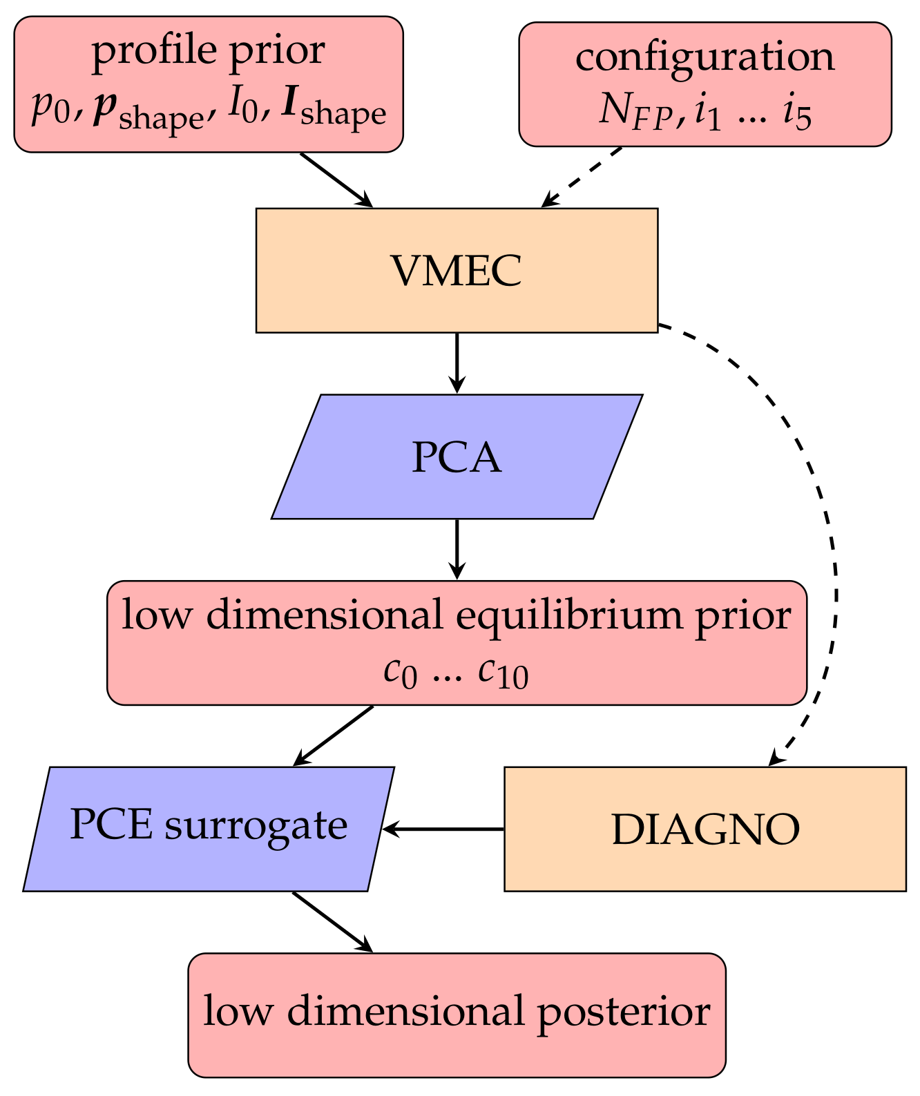
Scheme 1. Overview of the proposed framework.
Psf 09 00006 sch001
Figure 1. Samples drawn from the prior distribution of (left) the pressure profile shape and (right) the current profile shape.
Psf 09 00006 g001
Figure 2. Relative L 2 error of the low-dimensional equilibrium representation, evaluated for the samples from the prior.
Psf 09 00006 g002
Figure 3. Input pressure profile p compared with the pressure derived from p = J × B for a validation sample drawn from the prior and its low-dimensional representation.
Psf 09 00006 g003
Figure 4. Relative leave-one-out error ε l o o R of the polynomial chaos expansion surrogate models, mapping from the low-dimensional equilibrium parameters to the synthetic diagnostics.
Psf 09 00006 g004
Figure 5. One-dimensional projections of the low-dimensional equilibrium parameter prior distribution, kernel density estimation (KDE) and Laplace’s approximation of the posterior distribution.
Psf 09 00006 g005
Figure 6. Posterior samples of the flux surface geometry in comparison to the ground truth. The solid lines are linearly spaced contours of constant ρ , and the dashed lines are constant- θ contours.
Psf 09 00006 g006
Figure 7. Posterior kernel density estimation (KDE) of the total toroidal flux ( ψ 0 ).
Psf 09 00006 g007
Figure 8. Rotational transform profiles ι ρ drawn from the posterior distribution in comparison to the ground truth.
Psf 09 00006 g008
Figure 9. Pressure profiles calculated from the posterior using p = J × B together with the ground-truth pressure profile.
Psf 09 00006 g009
Table 1. The prior parameters and their distribution.
SymbolDistributionDescription
ψ 0 Uniform in 2.5 Wb , 1.6 Wb Total toroidal magnetic flux
p 0 Uniform in 0 , 200 kPa Pressure at the magnetic axis
p shape GP Minerva σ f = 1 λ core = 0.2 λ edge = 0.1 s 0 = 0.9 s w = 0.1 Pressure profile shape factors
reduced to 6 principal components
I 0 Uniform in 10 kA , 10 kA Total toroidal current
I shape GP RQ σ = 2 λ = 0.2 α = 2 Current profile shape factors
reduced to 3 principal components
Disclaimer/Publisher’s Note: The statements, opinions and data contained in all publications are solely those of the individual author(s) and contributor(s) and not of MDPI and/or the editor(s). MDPI and/or the editor(s) disclaim responsibility for any injury to people or property resulting from any ideas, methods, instructions or products referred to in the content.