Abstract
In this paper, we study the dynamical and statistical properties of the cosmic web and investigate their ability to infer the corresponding cosmological model. Our definition of the cosmic web is based on the local dimensionality of the gravitational collapse that classifies the cosmic web into four categories: voids, walls, filaments, and nodes. Our results show that each category has its specific non-Gaussian evolution over time and that these non-Gaussianities depend on the cosmological parameters. Nonetheless, the non-Gaussianities in each category exist even at early epochs when the matter field has a Gaussian distribution. Additionally, by using deep learning techniques, we show that leveraging the cosmic web information engenders an improved inference of cosmological parameters, when compared to merely using the matter field.
1. Introduction
The formation of structures in the Universe results from the highly non-linear dynamics (NLD) of gravitational collapse, and yields to a network (the cosmic web) of interconnected voids, sheets, filaments, and knots; thus, this web pattern ranges from large scales to small scales.
Previous works have shown that non-linearities depend on cosmology [1]; moreover, more recent studies [2] prove that combining the power spectra of the cosmic web categories improve the constraints on cosmological parameters. In addition, advances in N-body simulations allow for having access to a large set of cosmological models to finely study the non-linear evolution of the cosmic matter field. On the other hand, deep learning have improved their ability to learn from complex, non-linear data and they have been widely used in cosmology [3].
In this work, we use the large suite of Quijote simulations [4] to study the cosmic web properties, and we show using a deep neural network that they indeed allow for information beyond the matter field only, the paper is organised as follows: in Section 2 we describe our cosmic web segmentation technique, in Section 3 we illustrate the dynamical properties of the cosmic web environments and their dependence on the cosmological model, while, in Section 4, we present the results of the cosmological parameters inference using the cosmic web categories using a deep neural network. At the end, in Section 5, we discuss and explain the results; all the results of our study are presented in details in two forthcoming papers [5,6].
2. TWEB Algorithm
To characterize the cosmic web [7], we employ the algorithm proposed in [8], which is based on the local geometry of the collapse, in particular on the dimensionality that is quantified by the number of positive tidal field’s eigenvalues in each point. The tidal field is a hessian of the gravitational potential , and is computed from the smoothed matter density field by solving the Poisson equation on a regular grid using a Fast Fourier Transform.
The smooth density field is first computed by interpolating particles positions using a Cloud-in-Cell (CIC) interpolation scheme, on a regular grid of cells, then smoothed with a Gaussian kernel with a 2 Mpc·h radius.
Once the tidal field is computed, each grid point is classified as being a part of a node, filament, or wall, if it has, respectively, 3, 2, or 1 positive eigenvalues, while a grid point with no positive eigenvalue is a part of a void.
3. Cosmic Web Properties
3.1. Observables
Once each particle/grid cell has been assigned to an environment, we have a density field for each category, from which we can compute its probability density function , which is the number of grid cells between , and its power spectrum , the Fourier transform of the two-point correlation function. We can also compute scalar observables such as the moments or the mass- and volume-filling fractions in (i.e., how much mass/volume is occupied by a given category); in this section, we show the non-Gaussianities evolution in the cosmic web, and illustrate the cosmic web dependency on the cosmological parameters.
3.2. Data
To study the cosmic web properties, we use the Quijote suite of simulations [4], in particular the high-resolution fiducial model, with particles in a box of 1 (Gpc·h), and cosmological parameters for redshifts .
3.3. Non-Gaussianities
The PDF is a good tool to visualize the non-Gaussianities and their evolution in density distribution. Figure 1 shows that it is not possible to associate each category with a particular range of densities, since there is no unique density range for a particular category, but the density distribution of each category has its own evolution. For voids, the PDF becomes more shifted towards weak density regions, which can be understood by the fact that cosmic evolution implies more collapse of matter, which leaves more room for low densities, while it is the opposite for nodes, which can be understood by the same reason, since more collapse will generate denser regions; on the other side, walls, and filaments span a much larger range of densities, where walls shift for low densities and filaments towards high densities.
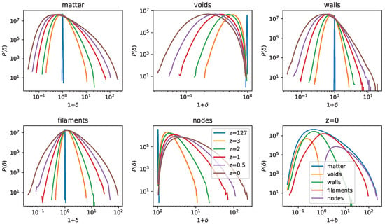
Figure 1.
Evolution wrt to the cosmic epoch of the probability density function of each cosmic web environment; the top left panel is for the whole matter field, while the bottom right panel is the of all categories at .
A more quantitative way to describe the PDFs behaviour is to look at the moments of the PDFs [9], such as the mean , the standard deviation , the skewness S, and kurtosis K defined, respectively, as:
The latter two moments quantify the asymmetry and flatness in the distribution, and they have zero values for a perfect Gaussian distribution.
Looking at the moments in Figure 2 highlight, in a more emphasized way, the non-Gaussianties evolution of each cosmic web category, and they provide a quantitative way to understand the non-Gaussianities in the initial density field, which is generated with Gaussian fluctuations; this is confirmed by its low skewness (), while, for the categories, they already have larger skewness, so their initial distributions are non-Gaussians, unlike the matter field.
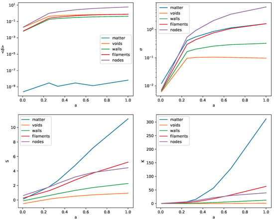
Figure 2.
Evolution of each of the four moments of the density field for each category wrt scale factor ; for the mean density, we plot the absolute value on a logarithmic scale, but the mean density for voids and walls are always negative.
The density means clearly show that the filaments and nodes evolve towards high-density regions, while the walls and voids shift towards the low-density regions, and it is remarkable that nodes and filaments are the most non-Gaussian categories since they have the largest skewness and kurtosis.
3.4. Cosmological Dependence of CW Environment
Another remarkable property of the cosmic web is its dependence on cosmological parameters; to account for this dependence, we use the 2000 Latin hypercube Quijote simulations, which have the same dynamical properties of the fiducial model but with varying cosmological parameters such that , , , , and . For each of the 2000 cosmologies, we compute the cosmic web categories at , and their corresponding observables. In Figure 3, we show some illustrations of some of the observables, and it clearly shows that the cosmic web properties, whether the geometrical (i.e., mass and volume fractions), or dynamical (moments) depend on the cosmological parameters. In addition, and appear to have the highest impact.
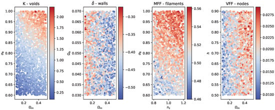
Figure 3.
Scatter plots of some cosmological parameters with colour maps corresponding to the values of the observable written on the top of each panel.
4. Cosmological Parameters Inference
The results in the previous section show the dependence of the cosmic web categories on the cosmological parameters, and they motivated us to investigate cosmological parameter extraction using the cosmic web properties.
4.1. Method
To perform the cosmological parameters’ inference, we employ a simple deep neural network, to predict the five cosmological parameters given a physical observable.
We train the network on 1800 simulations, and we test it on 200 simulations with cosmologies totally different from the ones it had trained on, the details of the architecture can be found in Appendix A.
As a physical observable to feed to the network, we use the power spectrum up to the Nyquist frequency = 3.2 h·Mpc; thus, our input is the power spectrum of a category (or a combination of categories) and our output layer is the five cosmological parameters.
4.2. Performance Evaluation and Results
To evaluate the performance for every parameter, we have two methods:
- Visually, by plotting a predicted vs. true value scatter plot: the less scattered around the identity line, the better the performance is (cf. Figure 4).
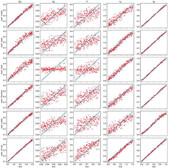 Figure 4. Ground truth vs. predicted values scatter plot; using the column, we can compare how the fit changes for one parameter using different categories. Horizontally, we can compare given category predictions for different parameters.
 - Quantitatively by computing the relative squared error where and are, respectively, the true and predicted parameter, and is the average of the true parameters; the RSE allows us to compare different inference results: the lower the RSE, the better the performance is (cf. Table 1).
 Table 1. Relative squared error for each cosmological parameter using different categories, the last line is when we combine all the categories, and we obtain the best results except for , the best results for each parameters are written in bold.
5. Discussion
The results show that, after segmenting the matter field into the four categories of the cosmic web, we obtain additional information of the dependence on the non-linear dynamics on the cosmological model. This is clearly shown in the results of Figure 3, which shows that different quantities of the cosmic web adopt different values when we change the cosmological parameters.
In addition, this was confirmed when we used deep neural networks to extract cosmological parameters using information from the cosmic web categories, in particular the power spectrum. This is shown in Table 1 where the RSE for each parameter is the lowest when we include all the cosmic web information, except for , which is best predicted by the filaments.
Moreover, looking vertically at Table 1 and Figure 4 demonstrates that every parameter is better predicted by a particular category; for instance, is better predicted by large-scale structures (voids and walls), and this can be understood since tilts the shape of the linear , which coincides with the full non-linear up to and corresponds to a large-scale structure such as walls and voids. For , the filaments appear to be the best tracers for it; this may imply that filaments span a scale that is in the order of the Baryon acoustic oscillations (≈100 Mpc·h), causing them to be the most sensitive to the density of baryons. The degradation of the accuracy of prediction when using all the categories combined can be justified by the fact that other categories (particularly the walls) are insensitive to , so they play the role of a redundant information for when combining all the power spectra.
On the other hand, and always have a low RSE; this is well in agreement with Figure 3, which shows that cosmic web properties have regular behaviour with respect to and .
Author Contributions
M.S. and J.-M.A. equally contributed to this work. All authors have read and agreed to the published version of the manuscript.
Funding
This research received no external funding.
Institutional Review Board Statement
Not applicable.
Informed Consent Statement
Not applicable.
Data Availability Statement
Not applicable.
Acknowledgments
This work was granted access to the HPC resources of IDRIS under the allocation 2022-[92287] made by GENCI.
Conflicts of Interest
The authors declare no conflict of interest.
Appendix A. DNN Architecture
We employ a multi-layers perceptron (MLP) architecture, and the architecture is:
- Input layer: working with one field, our input layer has 500 points (number of points); when we combine all the fields, we stack all the power spectra creating an input of 2500 points
- Hidden layers: In the case of one field, the hidden layers have 1024 neurones each; in the case of combined fields, we use hidden layers with 2048 neurones. We also use a dropout layer [10] of 0.3 rate between every two hidden layers; the number of hidden layers was individually tuned for every observable and is summarized in the table below.

Table A1.
Summarizing architecture for different observables, we employ Adam [11] optimizer.
Table A1.
Summarizing architecture for different observables, we employ Adam [11] optimizer.
| Observable | Hidden Layers | Learning Rate |
|---|---|---|
| —matter | 2 | 5 × 10 |
| —voids | 2 | 1 × 10 |
| —walls | 3 | 1 × 10 |
| —filaments | 3 | 5 × 10 |
| —nodes | 3 | 1 × 10 |
| —all | 3 | 1 × 10 |
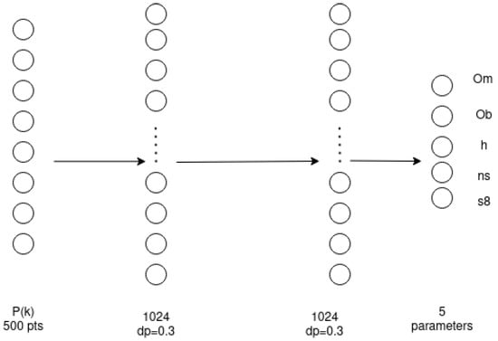
Figure A1.
Exampe of a network with two layers of 1024 neurones with a dropout rate of 0.3.
References
- Alimi, J.M.; Füzfa, A.; Boucher, V.; Rasera, Y.; Courtin, J. Imprints of dark energy on cosmic structure formation—I. Realistic quintessence models and the non-linear matter power spectrum. Mon. Not. R. Astron. Soc. 2010, 401, 775–790. [Google Scholar] [CrossRef]
- Bonnaire, T.; Aghanim, N.; Kuruvilla, J.; Decelle, A. Cosmology with cosmic web environments. Astron. Astrophys. 2022, 661, A146. [Google Scholar] [CrossRef]
- Lazanu, A. Extracting cosmological parameters from N-body simulations using machine learning techniques. J. Cosmol. Astropart. Phy. 2021, 2021, 039. [Google Scholar] [CrossRef]
- Villaescusa-Navarro, F.; Hahn, C.; Massara, E.; Banerjee, A.; Delgado, A.M.; Ramanah, D.K.; Charnock, T.; Giusarma, E.; Li, Y. Erwan Allys The quijote simulations. Astrophys. J. Suppl. Ser. 2020, 250, 2. [Google Scholar] [CrossRef]
- Alimi, J.-M.; Shalak, M. Pearson distribution as a phenomenological approach of non-linear cosmic matter field statistics. 2023; in preparation. [Google Scholar]
- Shalak, M.; Alimi, J.-M. Inference of cosmological parameters by using cosmic web with neural networks. 2023; in preparation. [Google Scholar]
- Libeskind, N.I.; Weygaert, R.v.; Cautun, M.; Falck, B.; Tempel, E.; Abel, T.; Alpaslan, M.; Aragoon-Calvo, M.A.; Forero-Romero, J.E.; Gonzalez, R.; et al. Tracing the cosmic web. Mon. Not. R. Astron. Soc. 2018, 473, 1195–1217. [Google Scholar] [CrossRef]
- Hahn, O.; Porciani, C.; Carollo, C.M.; Dekel, A. Properties of dark matter haloes in clusters, filaments, sheets and voids. Mon. Not. R. Astron. Soc. 2007, 375, 489. [Google Scholar] [CrossRef]
- Einasto, J.; Klypin, A.; Hutsi, G.; Liivamagi, L.J.; Einasto, M. Evolution of skewness and kurtosis of cosmic density fields. Astron. Astrophys. 2021, 652, A94. [Google Scholar] [CrossRef]
- Srivastava, N.; Hinton, G.; Krizhevsky, A.; Sutskever, I.; Salakhutdinov, R. Dropout: A simple way to prevent neural networks from overfitting. J. Mach. Learn. Res. 2014, 15, 1929–1958. [Google Scholar]
- Kingma, D.P.; Ba, J. Adam: A Method for Stochastic Optimization. arXiv 2014, arXiv:1412.6980. [Google Scholar]
Disclaimer/Publisher’s Note: The statements, opinions and data contained in all publications are solely those of the individual author(s) and contributor(s) and not of MDPI and/or the editor(s). MDPI and/or the editor(s) disclaim responsibility for any injury to people or property resulting from any ideas, methods, instructions or products referred to in the content. |
© 2023 by the authors. Licensee MDPI, Basel, Switzerland. This article is an open access article distributed under the terms and conditions of the Creative Commons Attribution (CC BY) license (https://creativecommons.org/licenses/by/4.0/).