Abstract
The simplest Bayesian system used to illustrate ideas of probability theory is a coin and a boolean utility function. To illustrate ideas of hypothesis testing, estimation or optimal control, one needs to use at least two coins and a confusion matrix accounting for the utilities of four possible outcomes. Here we use such a system to illustrate the main ideas of Stratonovich’s value of information (VoI) theory in the context of a financial time-series forecast. We demonstrate how VoI can provide a theoretical upper bound on the accuracy of the forecasts facilitating the analysis and optimization of models.
1. Introduction
The concept of value of information has different definitions in the literature [1,2]. Here we follow the works of Ruslan Stratonovich and his colleagues, who were inspired by Shannon’s work on rate distortion [3] and made a number of important developments in the 1960s [2]. These mainly theoretical results are gaining new interest thanks to the advancements in data science and machine learning and the need for a deeper understanding of the role of information in learning. We shall review the value of information theory in the context of optimal estimation and hypothesis testing, although the context of optimal control is also relevant.
Consider a probability space and a random variable (a measurable function). The optimal estimation of is the problem of finding an element maximizing the expected value of some utility function (or minimizing for cost ). The optimal value is
where zero designates the fact that no information about the specific value of is given, only the prior distribution . At the other extreme, let be another random variable that communicates full information about each realization of x. This entails that there is an invertible function such that is determined uniquely by the ‘message’ . The corresponding optimal value is
where an optimal y is found for each z (i.e., optimization over all mappings ). In the context of estimation, variable x is the response (i.e., the variable of interest) and z is the predictor. The mapping represents a model with output .
Let be the intermediate amounts of information, and let be the corresponding optimal values. The value of information is the difference [4]:
There are, however, different ways in which the information amount I and the quantity can be defined, leading to different types of the value function . For example, consider a mapping with a constraint on the cardinality of its image. The mapping f partitions its domain into a finite number of subsets . Then, given a specific partition , one can find optimal maximizing the conditional expected utility for each subset . This optimization should be repeated for different partitions , and the optimal value is defined over all partitions , satisfying the cardinality constraint :
Here, . The quantity is called Hartley’s information, and the difference in this case is the value of Hartley’s information. One can relax the cardinality constraint and replace it with the constraint on entropy , where . In this case, is called the value of Boltzmann’s information [4].
One can see from Equation (1) that the computation of the value of Hartley’s or Boltzmann’s information is quite demanding and may involve a procedure such as the k-means clustering algorithm or training a multilayer neural network. Thus, using these values of information is not practical due to high computational costs. The main result of Stratonovich’s theory [4] is that the upper bound on Hartley’s or Boltzmann’s values of information is given by the value of Shannon’s information, and that asymptotically all these values are equivalent (Theorems 11.1 and 11.2 in [4]). The value of Shannon’s information is much easier to compute.
Recall the definition of Shannon’s mutual information [3]:
where is the joint probability distribution on , and is the conditional entropy. Under broad assumptions on the reference measures (see Theorem 1.16 in [4]), the following inequalities are valid:
The value of Shannon’s information is defined using the quantity:
The optimization above is over all conditional probabilities (or joint measures ) satisfying the information constraint . Contrast this with for Hartley’s or Boltzmann’s information (1), where optimization is over the mappings . As was pointed out in [5], the relation between functions (1) and (2) is similar to that between optimal transport problems in the Monge and Kantorovich formulations. Joint distributions optimal in the sense of (2) are found using the standard method of Lagrange multipliers (e.g., see [4,6]):
where parameter , called temperature, is the Lagrange multiplier associated with the constraint . Distributions P and Q are the marginals of W, and function is defined by normalization . In fact, taking partial traces of solution (3) gives two equations:
Equation (5) defines function . If the linear transformation has an inverse, then from Equation (4) one obtains or
where , is the kernel of the inverse transformation , and is random entropy or surprise. Integrating the above with respect to measure we obtain
where . Function is the cumulant generating function of optimal distribution (3). Indeed, the expected utility and Shannon’s information for this distribution are
The first formula can be obtained directly by differentiating , and the second by substitution of (3) into the formula for Shannon’s mutual information. Function is clearly the conditional entropy because .
Note that information is the Legendre–Fenchel transform of convex function (indeed, ). The inverse of is the optimal value from Equation (2) defining the value of Shannon’s information, and it is the Legendre–Fenchel transform of concave function , which is called free energy.
The general strategy for computing the value of Shannon’s information is to derive the expressions for and from function (alternatively, one can obtain and from free energy ). Then the dependency is obtained either parametrically or by excluding . Let us now apply this to the simplest case.
2. Value of Shannon’s Information for the System
Let , and let be the utility function, which we can represent by a matrix:
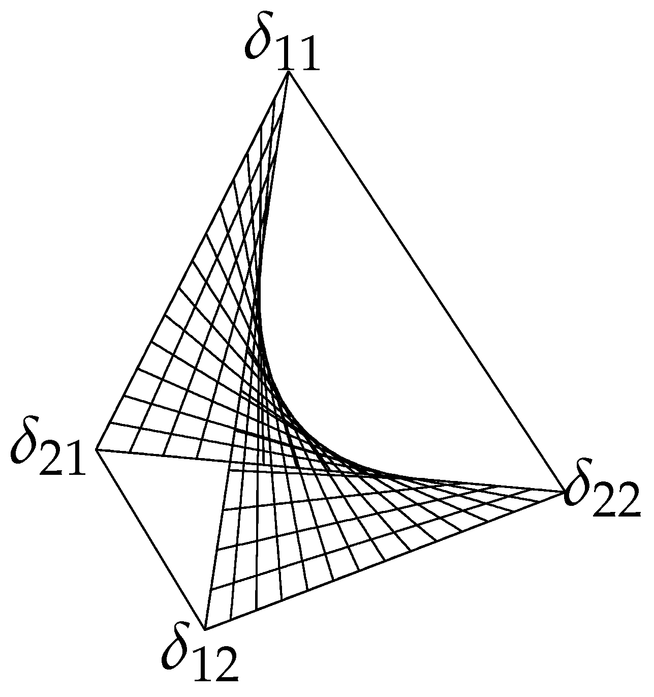
It is called the confusion matrix in the context of hypothesis testing, where rows correspond to the true states , and columns correspond to accepting or rejecting the hypothesis . The set of all joint distributions is a 3-simplex (tetrahedron), shown in Figure 1. The 2D surface in the middle is the set of all product distributions , which correspond to the minimum of mutual information (independent ). With no additional information about x, the decision to accept or to reject the hypothesis is completely determined by the utilities and prior probabilities and . Thus, one has to compare expected utilities and . The output distribution is an elementary -distribution:

Figure 1.
A 3-simplex of all joint distributions on a system.
The optimal value corresponding to information is . In the case when and , the condition for is and . With and , the value represents the best possible accuracy for prior probabilities . If additional information about x is communicated, say by some random variable , then the maximum possible improvement is the value of this information. The first step in deriving function for the value of Shannon’s information (2) is to obtain the expression for function .
Writing Equation (4) in the matrix form and using the inverse matrix gives the solution for function :
where . This gives two equations:
Therefore, the expression for function is
Its first derivative gives the expression for :
The expression for information is obtained from , where . Two functions and define parametric dependency for the value of Shannon’s information (2).
Notice that function (and hence and ) depends in general on . If, however, and , then, using the formula , we obtain simplified expressions: and
Let us denote . Then the expression for information is
In the first step we used the formulae and . The last equation is written using binary entropies , which shows that an increase of information in a binary system is directly related to an increase of the probability due to conditioning on the ‘message’ about the realization of . Additionally, substituting we obtain the closed-form expression:
Let us derive the equations for the output probabilities . This can be done using Equation (5), which in the matrix form is . Thus, we obtain
where . This gives two equations:
It is easy to check that . Additionally, if , then and for all . However, when , there exists such that either or for . The value can be found from or . For this value is
One can show that and . Thus, the output probabilities are non-negative for all , which corresponds to positive information and .
It is important to note that in the limit , corresponding to an increase of information to its maximum, the output probabilities converge to .
3. Application: Accuracy of Time-Series Forecasts
In this section, we illustrate how the value of information can facilitate the analysis of the performance of data-driven models. Here we use financial time-series data and predict the signs of future log returns. Thus, if and are prices of an asset at two time moments, then is the log-return at t. The models will try to predict whether the future log return is positive or negative. Thus, we have a system, where is the true sign, and is the prediction. The accuracy of different models will be evaluated against the theoretical upper bound, defined by the value of information.
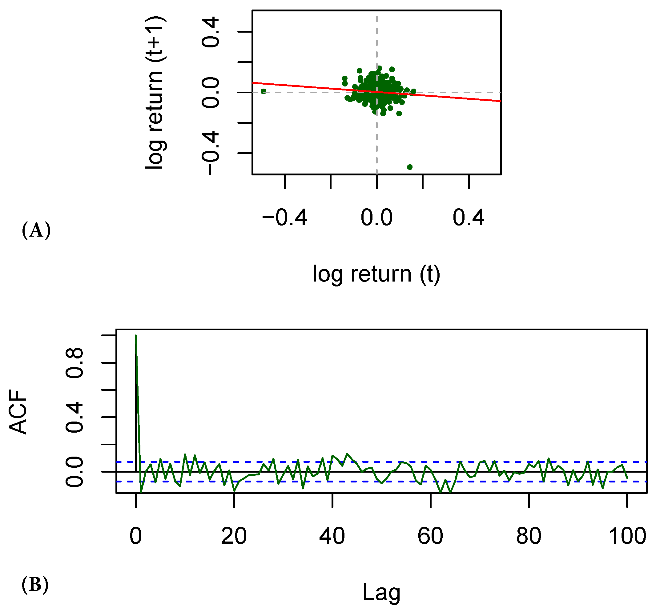
The data used here are from the set of close-day prices of several cryptocurrency pairs between 1 January 2019 and 11 January 2021. Figure 2 shows the price of Bitcoin against USD (left) and the corresponding log returns (right). Predicting price changes is very challenging. In fact, in economics, log returns are often assumed to be independent (and hence prices are assumed to be Markov). Indeed, one can see no obvious relation on the left chart on Figure 3, which plots logreturns (abscissa) and (ordinates). In reality, however, some amounts of information and correlations exist, which can be seen from the plot of the autocorrelation function for BTC/USD shown on the right chart of Figure 3.

Figure 2.
Close day prices of BTC/USD (left) and the corresponding log returns (right).
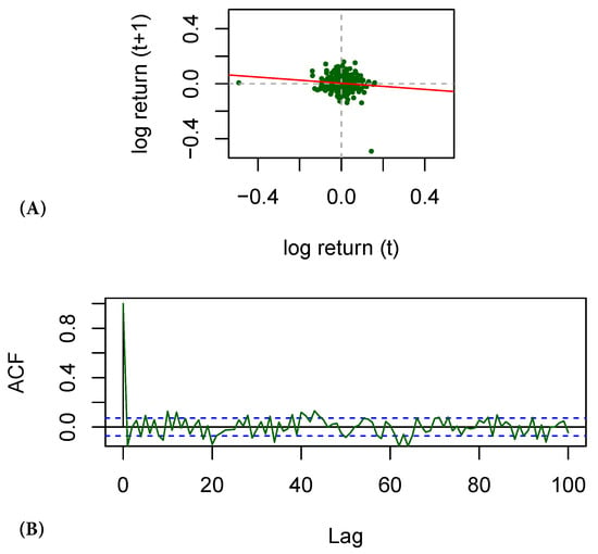
Figure 3.
Log returns of BTC/USD on two consecutive days (A); the autocorrelation function (B).
The idea of autoregressive models is to use the small amounts of information between the past and future values for forecasts. In addition to autocorrelations (correlations between the values of at different times), information can be increased by using cross-correlations (correlations between log-returns of different symbols in the dataset). Thus, the vector of predictors used here is an -tuple, where m is the number of symbols used, and n is the number of time lags. In this paper, we report the results of models using the range of symbols (BTC/USD, ETH/USD, DAI/BTC, XRP/BTC, IOT/BTC) and of lags. This means that the models used predictors , where ranged from 2 to 100. The model output is the forecast of the sign (the response) of future log return of BTC/USD. Here we report results from the following models:
- Logistic regression (LM). This model has no hyperparameters.
- Partial least squares discrimination (PLSD). We used the SIMPLS algorithm [7] with three components.
- Feed-forward neural network (NN). Here we used one hidden layer with three logistic units.
In order to analyse the performance of models using the value of information, one has to estimate the amount of information between the predictors and the response variable x. Here we employ two methods. The first uses the following Gaussian formula [4]:
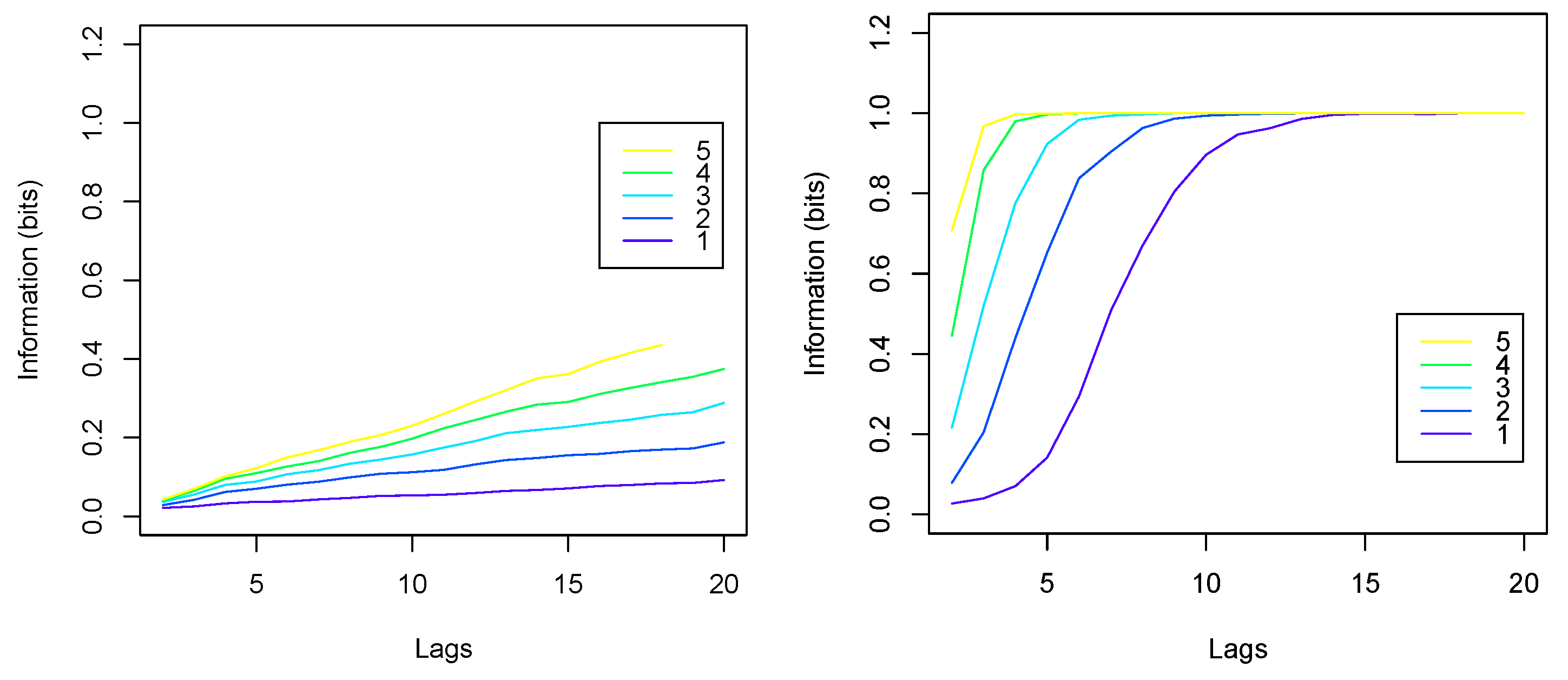
where are the covariance matrices. Because the distributions of log returns are generally not Gaussian, this formula is an approximation (in fact, it gives a lower bound). The second method is based on the discretization of continuous variables. Because models were used to predict signs of log returns, here we used discretization into two subsets. Figure 4 shows the average amounts of information in the training sets, computed using the Gaussian formula (left) and using binary discretization (right). Information (ordinates) is plotted against the number n of lags (abscissa) and for symbols (different curves). One can see that the amounts of information using Gaussian approximation (left) are generally lower than those using discretization (right). We note, however, that linear models can only use linear dependencies (correlations), which means that Gaussian approximation is sufficient for assessing the performance of linear models, such as LM and PLSD. Non-linear models, on the other hand, can potentially use all information present in the data. Therefore, we used information estimated with the second method to assess the performance of NN.
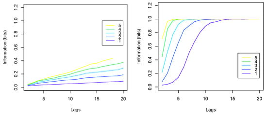
Figure 4.
The average amounts of mutual information between predictors and response in the training sets, computed using Gaussian approximation (left) and using binary discretization (right). The abscissa shows the numbers n of lags; different curves correspond to numbers m of symbols used.
For each collection of predictors and response x, the data were split into multiple training and testing subsets using the following rolling window procedure: we used 200- and 50-day data windows for training and testing, respectively; after training and testing the models, the windows were moved forward by 50 days and the process repeated. Thus, the data of approximately 700 days (January 2019 to January 2021) were split into pairs of training and testing sets. The results reported here are the average of results from these 10 subsets.
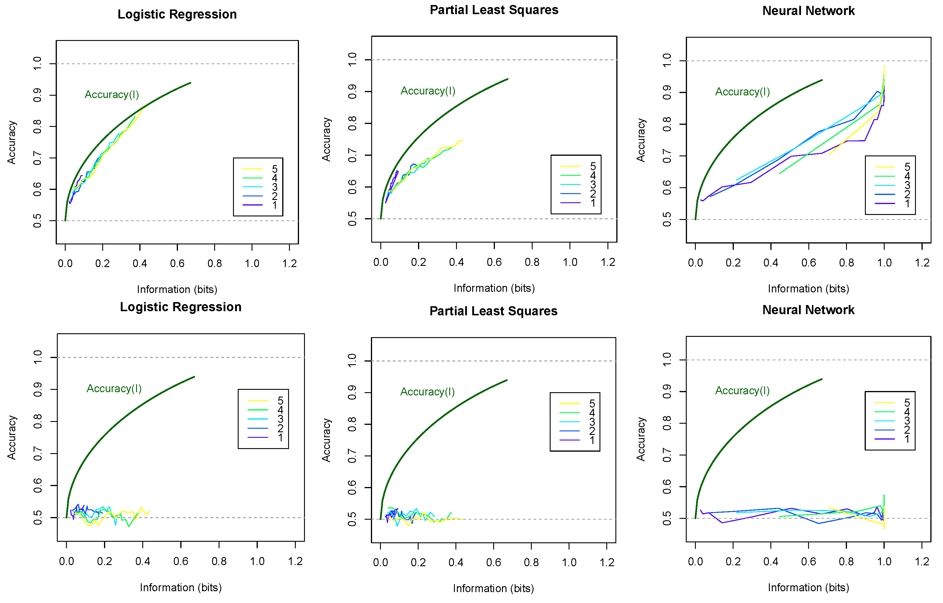
Figure 5 shows the accuracies of models plotted against information amounts I in the training data. The top row shows results on the training sets (i.e. fitted values) and the bottom row for new data (i.e., predicted values). Different curves are plotted for different numbers of symbols . The theoretical upper bounds are shown by the curves computed using the inverse of function (6) with and . Here we note the following observations:
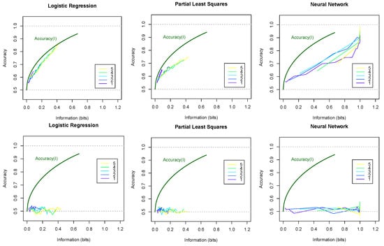
Figure 5.
Accuracy of fitted values on training data (top row) and of predicted values on testing data (bottom row) for three types of models plotted as functions of information in the training data. Theoretical curves are plotted using the inverse of function (6) for and . Different curves correspond to the number m of symbols used.
- The accuracy of fitting the training data closely follows theoretical curve . The accuracy of predicting new data (testing sets) is significantly lower.
- Increasing information increases the accuracy on training data, but not necessarily on new data.
- Models using symbols appear to achieve better accuracy than models using symbol with the same amounts of information. Thus, surprisingly, cross-correlations potentially provide more valuable information for forecasts than autocorrelations.
4. Discussion
We have reviewed the main ideas of Stratonovich’s value of information theory [2,4] and applied it to the simplest Bayesian system. We explicitly performed the main computations for the cumulant generating function and derived functions and defining the dependency and the value of Shannon’s information . The main application of the considered binary example the is evaluation of the accuracy of model predictions or hypothesis testing. The analysis the of performance of data-driven models can be enriched by the use of the value of information. However, one needs to be careful about the estimation of the amount of information in the data. Gaussian approximation of mutual information can be used for linear models. However, other techniques should be used for the analysis of non-linear models, such as neural networks. Here we applied the value of information to the analysis of financial time-series forecasts. These methods can be generalized to many other machine learning and data science problems.
Author Contributions
Conceptualization and formal analysis, R.B.; methodology, R.B., P.P. and J.P.; software, R.B.; modelling and experiments, R.B.; data curation, R.B., P.P. and J.P.; writing—original draft preparation, R.B.; writing—review and editing, R.B., P.P. and J.P.; funding acquisition, J.P. All authors have read and agreed to the published version of the manuscript.
Funding
This research was funded in part by the ONR grant number N00014-21-1-2295.
Institutional Review Board Statement
Not applicable.
Informed Consent Statement
Not applicable.
Data Availability Statement
Close day prices used in this work are available at https://doi.org/10.22023/mdx.21436248.
Acknowledgments
Stefan Behringer is deeply acknowledged for additional discussion of the example, and Roman Tarabrin is deeply acknowledged for providing a MacBookPro laptop used for the computational experiments.
Conflicts of Interest
The authors declare no conflict of interest.
References
- Howard, R.A. Information Value Theory. IEEE Trans. Syst. Sci. Cybern. 1966, 2, 22–26. [Google Scholar] [CrossRef]
- Stratonovich, R.L. On value of information. Izv. USSR Acad. Sci. Tech. Cybern. 1965, 5, 3–12. (In Russian) [Google Scholar]
- Shannon, C.E. A mathematical theory of communication. Bell Syst. Tech. J. 1948, 27, 379–423 and 623–656. [Google Scholar] [CrossRef]
- Stratonovich, R.L. Theory of Information and Its Value; Springer: Cham, Switzerland, 2020. [Google Scholar]
- Belavkin, R.V. Relation Between the Kantorovich-Wasserstein Metric and the Kullback-Leibler Divergence. In Proceedings of the Information Geometry and Its Applications, Liblice, Czech Republic, 12–17 June 2016; Ay, N., Gibilisco, P., Matúš, F., Eds.; Springer International Publishing: Cham, Switzerland, 2018; pp. 363–373. [Google Scholar]
- Belavkin, R.V. Optimal measures and Markov transition kernels. J. Glob. Optim. 2013, 55, 387–416. [Google Scholar] [CrossRef]
- de Jong, S. SIMPLS: An alternative approach to partial least squares regression. Chemom. Intell. Lab. Syst. 1993, 18, 251–263. [Google Scholar] [CrossRef]
Publisher’s Note: MDPI stays neutral with regard to jurisdictional claims in published maps and institutional affiliations. |
© 2022 by the authors. Licensee MDPI, Basel, Switzerland. This article is an open access article distributed under the terms and conditions of the Creative Commons Attribution (CC BY) license (https://creativecommons.org/licenses/by/4.0/).

