Abstract
Bayesian analysis is particularly useful for inferring models and their parameters given data. This is a common task in metabolic modeling, where models of varying complexity are used to interpret data. Nested sampling is a class of probabilistic inference algorithms that are particularly effective for estimating evidence and sampling the parameter posterior probability distributions. However, the practicality of nested sampling for metabolic network inference has yet to be studied. In this technical report, we explore the amalgamation of nested sampling, specifically diffusive nested sampling, with reversible jump Markov chain Monte Carlo. We apply the algorithm to two synthetic problems from the field of metabolic flux analysis. We present run times and share insights into hyperparameter choices, providing a useful point of reference for future applications of nested sampling to metabolic flux problems.
1. Introduction
Developing a quantitative understanding of the metabolic processes that convert substrates into useful products is essential for bioprocess development and metabolic engineering. Metabolic network models have proven to be effective in describing metabolic processes in a wide range of contexts [1,2,3]. Although metabolic network models are mainly based on biochemical knowledge, the process of reconstructing them introduces uncertainty into the model formulation [4]. Broadly, the following two types of uncertainty are prevalent:
- Structural uncertainty—introduced, for example, by gap-filling heuristics or by unknown regulation mechanisms;
- Operational uncertainty—for instance, even when “complete” structural knowledge is available, gene expression levels, enzyme activities and metabolic concentrations depend on the in vivo conditions applied, which may cause the catalyzed reactions or whole pathways to operate at different capacities or even in reverse.
The first type of uncertainty, structural uncertainty, results in a variety of metabolic network models that differ in terms of the number of parameters and, consequently, dimensionality. Operational uncertainty, on the other hand, corresponds to uncertainty in the values of the metabolic parameters for each network model. Structural and operational uncertainty are inherently coupled and must be addressed concurrently. In this setting, we refer to the process of inferring the implied network structure and its corresponding model parameters as metabolic network inference.
We use Bayesian statistics to infer the metabolic parameters along with the metabolic network model. Given the data D, the posterior of the parameters, the metabolic fluxes , is determined using Bayes’ theorem
where is the flux prior, is the likelihood, and is the evidence (or marginal likelihood). All these quantities are defined with respect to the metabolic network model . An example network model for Escherichia coli is shown in Figure 1.
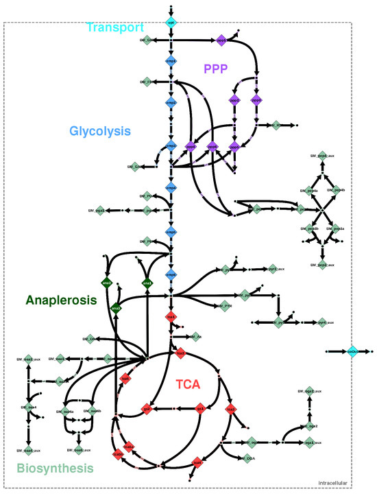
Figure 1.
Metabolic network model instance for E. coli, adapted from [5]. Metabolic reactions are visualized by diamonds. Nominal reaction directions are indicated by bold arrows; double-headed arrows indicate that two flux parameters are associated with the reaction, whereas the remaining reactions are accompanied by a single flux parameter. The diamonds are color-coded according to the metabolic pathway.
The evidence represents the probability of generating observations from the metabolic model , and is, thus, the central quantity for comparing alternative models [6,7]. The evidence is defined by the integral of the likelihood, weighted by the prior over the flux parameters
In any realistic case, the integral in Equation (2) needs to be solved numerically. Because metabolic network models are high-dimensional, computing the model evidence of a metabolic model is computationally challenging and requires probabilistic methods to alleviate the curse of dimensionality. An additional challenge in calculating is when the posterior is multimodal, which is unknown beforehand. Indeed, multimodal posterior probability distributions have been observed for metabolic network models [8].
Nested sampling (NS) is a prominent class of Monte Carlo algorithms for estimating the model evidence and the parameter posterior probability [9,10,11]. The basic idea behind NS is to transform the evidence integral in Equation (2) into a one-dimensional integral of the likelihood over the enclosed prior mass. To this end, points, referred to as “particles”, are generated in the parameter space and evolved through regions of increasing likelihood, thereby exploring regions of decreasing prior mass. The NS algorithm stops evolving the particles once the contribution of the remaining prior mass and likelihood to the evidence becomes negligible. Finally, the model evidence is obtained by numerically solving the one-dimensional integral. Several variants of NS have been developed [12,13,14,15,16,17] and successfully applied in various contexts.
In this technical report, we show how NS can be used to sample the flux parameter posterior and compute evidence for metabolic network models that differ due to uncertainty in the model formulation. We build upon a combination of flux sampling [18] and trans-dimensional sampling using reversible jump MCMC (RJMCMC) [19] to evolve the particles. Importantly, RJMCMC is used to marginalize over metabolic models of different dimensions that share the same overall network structure. The algorithm has been successfully applied to metabolic network models in practice [8,20]. To estimate the model evidence for models with differing structure, we use trans-dimensional diffusive nested sampling (TDNS) [21,22]. TDNS is a combination of a trans-dimensional MCMC algorithm, in our case RJMCMC, and diffusive NS [23]. In contrast to classical NS, where particles explore the prior constrained by strictly increasing the likelihood levels, diffusive NS allows particles to “diffuse” back to lower likelihood levels, thereby allowing particles to move between modes. We compare the outcome of applying TDNS to two synthetic problems from the field of metabolic flux analysis. Special focus is on the diagnostic plots. We report TDNS hyperparameters used as reference for future application of TDNS in this field.
2. Materials and Methods
2.1. 13C Metabolic Flux Analysis
In 13C metabolic flux analysis (MFA), isotope labeling experiments are performed to set up an inverse problem with the goal of quantifying the metabolic reaction rates (fluxes) at steady-state conditions. Network structures consist of a set of biochemical reactions that are associated with metabolic pathways (cf. Figure 1). Depending on the experimental conditions, the metabolic reactions operate in the forward direction only, or in the forward and backward directions simultaneously. Whether the reactions operate in the forward only or in the forward and backward directions has important implications for the propagation of isotope labeling through the network structure [24]. Reactions that operate only in the forward direction have one associated flux parameter, while reactions that operate in both directions have two flux parameters. Therefore, different model variants emerge that have to be inferred together with the associated flux parameters. For more details about metabolic flux modeling and 13C MFA, we refer the interested reader to [25].
2.2. Implementation
To evaluate the likelihood in 13C MFA, we require fast simulation of labeling data, given a network model and parameter values as input. For this, we use the high-performance simulator 13CFLUX [26]. Given a network structure, we infer the operation mode of the reactions using RJMCMC; see [27] for an example from metabolic network inference. To estimate the model evidence while simultaneously inferring the operation mode of the reactions, we use TDNS, by combining 13CFLUX with the high-performance C++ packages DNest4 [28] for diffusive NS and HOPS [29] for MCMC sampling in convex-constrained parameter spaces.
3. Results
3.1. Problem Statement
To study TDNS, we infer the net flux parameters from two synthetic labeling experiments generated using a realistic network model of E. coli [30], which we call the data-generating network. We refer to the two synthetic labeling experiments as “Experiment 1” and “Experiment 2”, respectively. The data-generating network and experimental setups are provided in FluxML format [31] in the supplementary materials. Based on the data-generating network, we create seven additional models by removing or adding pathways. The data-generating network is defined by a central set of reactions (“C”) and the two pathways, called “E” and “G”. In addition to “E” and “G”, we consider a third pathway “M”, giving a set of eight structurally different models. Biologically, “E” is the Entner–Doudoroff pathway, “G” the glyoxylate shunt, and “M” the methylglyoxal pathway. For E. coli, “G” has been observed to be active, the activity of “E” depends on the environmental conditions, and “M” is typically inactive [32,33]. We denote the network models by a letter combination. The data-generating model is denoted “C-E-G”. The network models have between 6 and 9 net flux parameters and between 0 and 26 uncertain flux parameters originating from operational model uncertainty.
3.2. TDNS Hyperparameters, Diagnostics and Run Times
The two experiments and eight network structures result in a total of 16 TDNS runs. We ran the 16 instances of TDNS in parallel on eight CPUs, each with 16 cores and 32 threads. All runs were started and stopped simultaneously. As recommended by Ashton et al. [10], we report the estimated evidences, Kullback–Leibler (KL) divergences from prior to posterior, effective sample sizes (ESS), as well as the used CPUs and run time in Figure 2. Note that ESS is estimated differently in MCMC (autocorrelation) and NS (posterior weights). In this work, we report the ESS based on the NS estimator. In each case, the uncertainties for the evidences and KL divergences, estimated using DNest4, were below 0.02%. TDNS relies on hyperparameters to ensure accurate and efficient computation. Therefore, we report these hyperparameters in Table 1 to serve as a reference for metabolic network inference. Finally, we diagnose the 16 TDNS runs by checking the prior mass compression between subsequent levels, the likelihood levels as a function of enclosed prior mass X, the Metropolis-Hastings acceptance rates for the MCMC that evolves the particles, and the posterior weights. Figure 3 shows the results. Based on these diagnostics, we conclude that it is unlikely that we overlooked parameter regions contributing to the posterior, as the likelihood levels remain nearly constant when the prior mass is enclosed in gradually smaller regions.
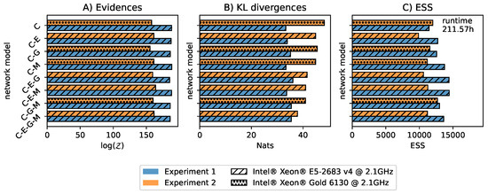
Figure 2.
For each model variant, we show the (A) model evidences, (B) Kullback-Leiber (KL) divergences from prior to posterior, and (C) effective sample size (ESS) as defined for NS. In contrast to classical NS, computing the uncertainty for the model evidences and KL divergences in diffusive NS is not straightforward [10,28]. We estimated the uncertainties for the model evidences and KL divergences by resampling the level compression 100 times, as implemented in DNest4. The relative uncertainties for the evidences and KL divergences estimated by DNest4 were below 0.02%.

Table 1.
TDNS hyperparameters for Experiments 1 and 2. See [28] for an in-depth description and explanation of the parameters. We manually tuned the maximum number of levels and new level intervals using exploratory runs. The diffusive NS parameters and were set according to the advice in [28]. The RJMCMC parameters were the step size of the parameter space proposals, the probability of proposing a new model instead of a parameter space proposal (model jump ratio), and the probability of switching a flux parameter on or off.
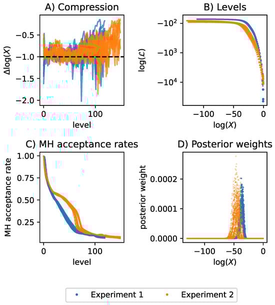
Figure 3.
Diagnostic plots for TDNS applied to Experiment 1 and Experiment 2. (A) The compression is defined as the logarithmic difference in enclosed prior mass X between adjacent likelihood levels. The target-compression was set to the Euler number e. Especially towards the higher levels, the compression was often low with respect to the target-compression, meaning that levels were created too closely. Low compression indicates computational overhead. (B) The created likelihood levels as a function of the enclosed prior mass X. We plot the log likelihood on a log-scale to highlight the difference in levels between both experiments. (C) Metropolis-Hastings (MH) acceptance rate of the MCMC proposals that evolve the particles. Towards higher levels, the acceptance rate declines, because it becomes harder and harder to generate proposals within the prior regions enclosed by higher and higher likelihood levels. If the acceptance rate reaches 0 before the bulk of the posterior is found, TDNS is stuck. Interestingly, for all runs of Experiment 2, there is a bulge in the decline of the acceptance rate. (D) In the plot of the posterior weights over the enclosed prior mass X, the posterior weights tend to 0 as X decreases, indicating that the bulk of the posterior mass was found for both experiments and all models.
3.3. Metabolic Network Inference Results
The model and parameter inferences for Experiments 1 and 2 are shown in Figure 4. Notably, the data-generating model “C-E-G” was not assigned a high probability in either experiment. Experiment 1 did not assign a high probability to any specific model. In contrast, Experiment 2 classified the “C-G” model as the most likely one, and the alternative models that contain pathway “G” together accounted for 90.08% of the evidence. Therefore, Experiment 2 identified pathway “G” with high certainty. The failure of Experiment 1 to find “G” was due to the uninformative input substrate, which resulted in measurements that were uninformative with respect to the presence of “G”. By contrast, pathway “E” was not detected at all and accounted for only around 6.7% of the evidence. It is not surprising that the experiments failed to find all pathways, as it has been demonstrated for E. coli that even the combination of several 13C MFA datasets is often insufficient to accurately resolve all net fluxes and pathways [30]. Independently of the detected pathways, the marginal posteriors for the central net fluxes (i.e., the fluxes belonging to “C”) show substantial posterior overlap across network structures. In other words, although specific pathways were difficult to infer from the data, the central net fluxes were recovered.
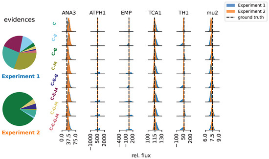
Figure 4.
Relative model evidences for each pathway combination and inferences for net fluxes that are shared between all metabolic network structures. The net fluxes are given relative to the input flux of 100 mmol/gCWD/h. Strikingly, the different network models agreed well on the central fluxes for Experiment 2.
4. Discussion
In this technical report, we compared the outcomes of applying TDNS to two synthetic experiments from the field of 13C MFA. The synthetic experiments reflect a common challenge of real-word 13C MFA, namely that the data are insufficient to fully resolve the underlying metabolic network structure. Nevertheless, the central fluxes were recovered.
TDNS has several hyperparameters that influence computational performance and the reliability of evidence estimates and posterior samples. For example, hyperparameter tuning includes setting an appropriate maximum number of levels to avoid creating computationally costly levels that do not contribute significantly to the posterior. Exploratory runs of TDNS were performed beforehand to find suitable hyperparameters. Moreover, Brewer and Foreman-Mackey [28] argue that skipping step size tuning and using heavy-tailed proposal moves for evolving particles is often more robust and simpler than adjusting the proposal moves. In our application, we found that tuning the step size of the proposals was required to maintain non-zero acceptance rates at higher likelihood levels. Therefore, we report our hyperparameters and diagnostics for future reference, especially as problems with similar KL divergences are expected to require similar computational effort [34]. In summary, improved hyperparameter tuning has the potential to make TDNS more efficient and robust for applications within and beyond the field of 13C MFA.
Author Contributions
Conceptualization, J.F.J. and K.N.; methodology, J.F.J.; software, J.F.J.; validation, J.F.J.; investigation, J.F.J.; writing—original draft preparation, J.F.J.; writing—review and editing, J.F.J., W.W., and K.N.; visualization, J.F.J.; supervision, K.N.; All authors have read and agreed to the published version of the manuscript.
Funding
This work was performed as part of the Helmholtz School for Data Science in Life, Earth and Energy (HDS-LEE) and received funding from the Helmholtz Association of German Research Centres.
Institutional Review Board Statement
Not applicable.
Informed Consent Statement
Not applicable.
Data Availability Statement
Models and code are publicly available at GitHub as part of the repository https://github.com/JuBiotech/Supplement_to_Jadebeck_et_al._MaxEnt_2024.
Acknowledgments
We thank Axel Theorell for inspiring discussions about RJMCMC for metabolic networks.
Conflicts of Interest
The authors declare no conflicts of interest.
References
- Orth, J.D.; Thiele, I.; Palsson, B.Ø. What is flux balance analysis? Nat. Biotechnol. 2010, 28, 245–248. [Google Scholar] [CrossRef]
- Wiechert, W. 13C metabolic flux analysis. Metab. Eng. 2001, 3, 195–206. [Google Scholar] [CrossRef] [PubMed]
- Saa, P.A.; Nielsen, L.K. Formulation, construction and analysis of kinetic models of metabolism: A review of modelling frameworks. Biotechnol. Adv. 2017, 35, 981–1003. [Google Scholar] [CrossRef]
- Bernstein, D.B.; Sulheim, S.; Almaas, E.; Segrè, D. Addressing uncertainty in genome-scale metabolic model reconstruction and analysis. Genome Biol. 2021, 22, 64. [Google Scholar] [CrossRef]
- Theorell, A.; Jadebeck, J.F.; Wiechert, W.; McFadden, J.; Nöh, K. Rethinking 13C-metabolic flux analysis – the Bayesian way of flux inference. Metab. Eng. 2024, 83, 137–149. [Google Scholar] [CrossRef]
- Friel, N.; Wyse, J. Estimating the evidence—A review. Stat. Neerl. 2012, 66, 288–308. [Google Scholar] [CrossRef]
- Hoeting, J.A.; Madigan, D.; Raftery, A.E.; Volinsky, C.T. Bayesian model averaging: A tutorial. Stat. Sci. 1999, 14, 382–417. [Google Scholar] [CrossRef]
- Borah Slater, K.; Beyß, M.; Xu, Y.; Barber, J.; Costa, C.; Newcombe, J.; Theorell, A.; Bailey, M.J.; Beste, D.J.V.; McFadden, J.; et al. One-shot 13C15N-metabolic flux analysis for simultaneous quantification of carbon and nitrogen flux. Mol. Syst. Biol. 2023, 19, e11099. [Google Scholar] [CrossRef]
- Skilling, J. Nested sampling for general Bayesian computation. Bayesian Anal. 2006, 1, 833–859. [Google Scholar] [CrossRef]
- Ashton, G.; Bernstein, N.; Buchner, J.; Chen, X.; Csányi, G.; Fowlie, A.; Feroz, F.; Griffiths, M.; Handley, W.; Habeck, M.; et al. Nested sampling for physical scientists. Nat. Rev. Methods Prim. 2022, 2, 39. [Google Scholar] [CrossRef]
- Buchner, J. Nested sampling methods. Stat. Surv. 2023, 17, 169–215. [Google Scholar] [CrossRef]
- Handley, W.J.; Hobson, M.P.; Lasenby, A.N. polychord: Next-generation nested sampling. Mon. Not. R. Astron. Soc. 2015, 453, 4384–4398. [Google Scholar] [CrossRef]
- Trassinelli, M. Bayesian data analysis tools for atomic physics. Nucl. Instruments Methods Phys. Res. Sect. B Beam Interact. Mater. Atoms 2017, 408, 301–312. [Google Scholar] [CrossRef]
- Feroz, F.; Hobson, M.P.; Cameron, E.; Pettitt, A.N. Importance nested sampling and the MultiNest algorithm. Open J. Astrophys. 2019, 2. [Google Scholar] [CrossRef]
- Higson, E.; Handley, W.; Hobson, M.; Lasenby, A. Dynamic nested sampling: An improved algorithm for parameter estimation and evidence calculation. Stat. Comput. 2019, 29, 891–913. [Google Scholar] [CrossRef]
- Speagle, J.S. dynesty: A dynamic nested sampling package for estimating Bayesian posteriors and evidences. Mon. Not. R. Astron. Soc. 2020, 493, 3132–3158. [Google Scholar] [CrossRef]
- Buchner, J. UltraNest—A robust, general purpose Bayesian inference engine. J. Open Source Softw. 2021, 6, 3001. [Google Scholar] [CrossRef]
- Jadebeck, J.F.; Wiechert, W.; Nöh, K. Practical sampling of constraint-based models: Optimized thinning boosts CHRR performance. PLoS Comput. Biol. 2023, 19, e1011378. [Google Scholar] [CrossRef]
- Green, P.J. Reversible Jump Markov Chain Monte Carlo computation and Bayesian model determination. Biometrika 1995, 82, 711–732. [Google Scholar] [CrossRef]
- Mitosch, K.; Beyß, M.; Phapale, P.; Drotleff, B.; Nöh, K.; Alexandrov, T.; Patil, K.R.; Typas, A. A pathogen-specific isotope tracing approach reveals metabolic activities and fluxes of intracellular Salmonella. PLoS Biol. 2023, 21, e3002198. [Google Scholar] [CrossRef] [PubMed]
- Brewer, B.J. Inference for trans-dimensional Bayesian models with diffusive nested sampling. arXiv 2015, arXiv:1411.3921v3. [Google Scholar] [CrossRef]
- Brewer, B.J.; Huijser, D.; Lewis, G.F. Trans-dimensional Bayesian inference for gravitational lens substructures. Mon. Not. R. Astron. Soc. 2015, 455, 1819–1829. [Google Scholar] [CrossRef]
- Brewer, B.J.; Pártay, L.B.; Csányi, G. Diffusive nested sampling. Stat. Comput. 2010, 21, 649–656. [Google Scholar] [CrossRef]
- Wiechert, W.; Möllney, M.; Isermann, N.; Wurzel, M.; de Graaf, A.A. Bidirectional reaction steps in metabolic networks: III. Explicit solution and analysis of isotopomer labeling systems. Biotechnol. Bioeng. 1999, 66, 69–85. [Google Scholar] [CrossRef]
- Wiechert, W.; Nöh, K. Quantitative metabolic flux analysis based on isotope labeling. In Metabolic Engineering: Concepts and Applications; Nielsen, J., Stephanopoulos, G., Lee, S.Y., Eds.; Wiley: Weinheim, Germany, 2021; Chapter 3; pp. 73–136. [Google Scholar] [CrossRef]
- Weitzel, M.; Nöh, K.; Dalman, T.; Niedenführ, S.; Stute, B.; Wiechert, W. 13CFLUX2—High-performance software suite for 13C-metabolic flux analysis. Bioinformatics 2012, 29, 143–145. [Google Scholar] [CrossRef]
- Theorell, A.; Nöh, K. Reversible jump MCMC for multi-model inference in metabolic flux analysis. Bioinformatics 2019, 36, 232–240. [Google Scholar] [CrossRef]
- Brewer, B.J.; Foreman-Mackey, D. DNest4: Diffusive nested sampling in C++ and Python. J. Stat. Softw. 2018, 86, 1–33. [Google Scholar] [CrossRef]
- Jadebeck, J.F.; Theorell, A.; Leweke, S.; Nöh, K. HOPS: High-performance library for (non-) uniform sampling of convex-constrained models. Bioinformatics 2021, 37, 1776–1777. [Google Scholar] [CrossRef]
- Crown, S.B.; Long, C.P.; Antoniewicz, M.R. Integrated 13C-metabolic flux analysis of 14 parallel labeling experiments in Escherichia coli. Metab. Eng. 2015, 28, 151–158. [Google Scholar] [CrossRef] [PubMed]
- Beyß, M.; Azzouzi, S.; Weitzel, M.; Wiechert, W.; Nöh, K. The design of FluxML: A universal modeling language for 13C metabolic flux analysis. Front. Microbiol. 2019, 10, 1022. [Google Scholar] [CrossRef] [PubMed]
- Zamboni, N.; Fendt, S.M.; Rühl, M.; Sauer, U. 13C-based metabolic flux analysis. Nat. Protoc. 2009, 4, 878–892. [Google Scholar] [CrossRef] [PubMed]
- Antoniewicz, M.R. A guide to metabolic flux analysis in metabolic engineering: Methods, tools and applications. Metab. Eng. 2021, 63, 2–12. [Google Scholar] [CrossRef] [PubMed]
- Hu, Z.; Baryshnikov, A.; Handley, W. Aeons: Approximating the end of nested sampling. arXiv 2023, arXiv:2312.00294v1. [Google Scholar] [CrossRef]
Disclaimer/Publisher’s Note: The statements, opinions and data contained in all publications are solely those of the individual author(s) and contributor(s) and not of MDPI and/or the editor(s). MDPI and/or the editor(s) disclaim responsibility for any injury to people or property resulting from any ideas, methods, instructions or products referred to in the content. |
© 2025 by the authors. Licensee MDPI, Basel, Switzerland. This article is an open access article distributed under the terms and conditions of the Creative Commons Attribution (CC BY) license (https://creativecommons.org/licenses/by/4.0/).