Proceeding Paper

Inverse Bayesian Methods for Groundwater Vulnerability Assessment †

by
Nasrin Taghavi
1,*,
Robert K. Niven
1,
Matthias Kramer
1 and
David J. Paull
2
1
School of Engineering and Technology, The University of New South Wales, Canberra, ACT 2600, Australia
2
School of Science, The University of New South Wales, Canberra, ACT 2600, Australia
*
Author to whom correspondence should be addressed.
Presented at the 43rd International Workshop on Bayesian Inference and Maximum Entropy Methods in Science and Engineering, Ghent, Belgium, 1–5 July 2024.
Phys. Sci. Forum 2025, 12(1), 14; https://doi.org/10.3390/psf2025012014
Published: 5 November 2025

Abstract

Groundwater vulnerability assessment (GVA) is critical for understanding contaminant migration into groundwater systems, yet conventional methods often overlook its probabilistic nature. Bayesian inference offers a robust framework using Bayes’ rule to enhance decision-making through posterior probability calculations. This study introduces inverse Bayesian methods for GVA using spatial-series data, focusing on nitrate concentrations in groundwater as an indicator of groundwater vulnerability in agricultural catchments. Using the joint maximum a-posteriori (JMAP) and variational Bayesian approximation (VBA) algorithms, the advantages of the Bayesian framework over traditional index-based methods are demonstrated for GVA of the Burdekin Basin, Queensland, Australia. This provides an evidence-based methodology for GVA which enables model ranking, parameter estimation, and uncertainty quantification.

1. Introduction

In dynamical systems, the process of accurately determining the system function or model f from a set of discrete time series data [ x ( t 1 ) ,   x ( t 2 ) ,   x ( t 3 ) ,   ] is referred to as system identification [1,2]. The aim of this process is to establish the relationship between the observable state vector x ( t ) , which varies over time t, and the system function f . Sparse regression methods have been recently employed for system identification in dynamical and fluid flow systems [1,3,4]. These methods use regression to determine a matrix of coefficients which, when multiplied by a matrix of functional operations, reproduce the time series. Typically, a regularization technique is involved in the sparse regression process. However, selecting an appropriate regularization method can be challenging due to the heuristic or ad hoc nature of this choice, with little fundamental guidance available for selecting the appropriate method for any particular dataset [1,2,5,6,7].
To address this challenge, a Bayesian framework has been introduced for system identification using the Bayesian maximum a-posteriori (MAP) estimate [8]. Two Bayesian methods—joint maximum a-posteriori (JMAP) and variational Bayesian approximation (VBA)—have demonstrated numerous advantages [2]. These Bayesian algorithms can calculate the variances of inferred parameters, providing estimates of model errors. While JMAP and VBA Bayesian algorithms have been implemented for time-series data, their application to spatial-series data remains unexplored. One potential application of Bayesian methods on spatial-series data is the assessment of groundwater vulnerability within an aquifer. Groundwater vulnerability is defined as the probability of contaminants reaching a specific location within the groundwater system after being introduced at a point above the uppermost aquifer [9]. Groundwater vulnerability assessment (GVA) forms the conceptual base of groundwater protection plans [10].
Existing methods for GVA are either deterministic or based on empirical correlations, often neglecting the probabilistic nature of groundwater vulnerability [11]. The most commonly used GVA method is called the index-based DRASTIC method [12]. In this method, seven key input parameters are each assigned fixed weights and ordinal ratings, the latter derived from their measured values. These weights and ratings are combined to produce an overall weighted vulnerability index for each point, to quantify the potential for groundwater contamination. The higher the vulnerability index, the greater the potential for groundwater pollution. A modification of the DRASTIC method called the DRASTICL method has also been developed [13], adding a land use parameter to represent the influence of surface-based contaminant inputs.
Despite the widespread use of Bayesian inference in water resource modeling to analyze uncertainties [2,14,15,16,17,18,19,20,21], there is no application of inverse Bayesian methods for GVA. This study aims to fill this gap by applying inverse Bayesian methods to GVA using spatial-series data. Two iterative Bayesian algorithms, JMAP and VBA, are adapted for spatial-series data and subsequently compared with an index-based GVA method applied by [13] in the Burdekin Basin, Queensland, Australia. The study demonstrates that the Bayesian framework offers substantial advantages for GVA, providing an evidence-based methodology which enables model ranking, parameter estimation, and uncertainty quantification.

2. Theoretical Framework

This study proposes the application of inverse Bayesian methods for GVA using spatial-series data [22]. Measured nitrate concentrations in groundwater are treated as the dependent variable, serving as an indicator of vulnerability in agricultural catchments. The proposed model establishes a linear relationship between groundwater nitrate levels and a range of hydrogeological factors, expressed as:
C = Θ X Ξ + ϵ
where X denotes an m -dimensional spatial index, C represents an m -dimensional vector of nitrate concentrations (applied to each point X ), Θ represents an m × n matrix of hydrogeological variables (linked to X ), Ξ denotes an n -dimensional vector of model coefficients, and ϵ denotes an m -dimensional noise vector. In matrix-vector form, this can be written as:
C 1 C m = θ 1,1 θ 1 , n θ m , 1 θ m , n Ξ 1 Ξ n + ϵ 1 ϵ m .
In traditional index-based GVA methods such as DRASTIC (e.g., [12]), each parameter is assigned a weight and a rating based on their recognized significance or influence on groundwater vulnerability. The ratings are assigned using an ordinal scale for each parameter and organized as matrix Θ , whereas the weights represent predefined coefficient values from Ξ 1 to Ξ n . The resulting dependent variable generated by the method corresponds to the “vulnerability index”. This study extends beyond the conventional reliance on predetermined weights and ordinal ratings by estimating the vector Ξ , which most accurately reproduces the concentration vector C at observed locations when applied to the data Θ . This establishes a direct relationship between measured concentrations and model variables. The estimated coefficient vector Ξ ^ can then be applied to infer the nitrate concentration C ^ —as an indicator of groundwater vulnerability—at locations for which no observations are available.
Using Bayes’ theorem, the posterior probability of the model, Ξ , is derived from the observed data C [23]:
P Ξ C = P C Ξ   P Ξ P C P C Ξ   P Ξ
where P C Ξ represents the likelihood of C given Ξ , P Ξ represents the prior probability of Ξ , and P C represents the evidence for C . The maximum a-posteriori (MAP) point estimate of Ξ is then obtained by maximizing the posterior probability P Ξ C in its logarithmic form:
Ξ ^ = argmax Ξ [ ln P ( Ξ | C ) ] = argmax Ξ ln P C Ξ + ln P ( Ξ )
Assuming multivariate Gaussian noise with zero means and m × m covariance matrix V ϵ , and a multivariate Gaussian prior with zero means and n × n covariance matrix V Ξ , the MAP estimator Equation (4) transforms into:
Ξ ^ = argmax Ξ   ln exp 1 2 C Θ X Ξ V ϵ 1 2 + ln exp 1 2 Ξ V Ξ 1 2 = argmax Ξ   1 2 C Θ X Ξ V ϵ 1 2 1 2 Ξ V Ξ 1 2 = argmin Ξ   C Θ X Ξ V ϵ 1 2 + Ξ V Ξ 1 2
where, in general, a A 2 = a T A a is the LA norm of the vector a with A R . In Equation (5), C Θ X Ξ V ϵ 1 2 represents the Mahalanobis distance [24] associated with the likelihood term, while Ξ V Ξ 1 2 corresponds to the Mahalanobis distance of the prior. It is evident from Equation (5) that the Bayesian MAP leads to a minimization formulation defined by an objective function resembling that employed in regularization approaches. In this equation, the covariance matrices V ϵ of the noise and V Ξ of the prior are unknown. These can also be incorporated into the inferred posterior probability density function (pdf):
P Ξ , V ϵ , V Ξ C P C Ξ , V ϵ P Ξ V Ξ P V ϵ P V Ξ .
In the JMAP algorithm, Equation (6) is iteratively maximized considering Ξ , V ϵ , and V Ξ , to provide the estimated parameters Ξ ^ , V ϵ ^ , and V Ξ ^ . The VBA approach approximates the joint posterior through the separable formulation P Ξ , V ϵ , V Ξ C = q 1 Ξ q 2 V ϵ q 3 V Ξ and subsequently uses this approximation to define Ξ ^ , V ϵ ^ , and V Ξ ^ [8]. This approximation is achieved by optimizing q 1 Ξ , q 2 V ϵ , and q 3 V Ξ through minimization of the Kullback–Leibler divergence K = q ln q P d Ξ d V ϵ d V Ξ , where q denotes the approximated distribution and p the true value. In this study, q 1 Ξ is considered as a multivariate Gaussian distribution, while q 2 V ϵ and q 3 V Ξ are treated as inverse gamma distributions [8]:
q 1 Ξ = N Ξ μ Ξ , σ Ξ   q 2 V ϵ i = I G V ϵ i α i , β i q 3 V Ξ j = I G V Ξ j α j , β j
The parameters ( μ Ξ , σ Ξ ) , ( α i , β i ) , and α j , β j are updated within an inner iteration loop with constant values of α 0 and β 0 . Two iterative Bayesian algorithms, JMAP and VBA, were adapted for spatial-series data using a MATLAB structure derived from [2] for dynamical systems and integrated with a Bayesian inference code developed by [8]. The original algorithms allow for multidimensional data, whereas this study focuses on a one-dimensional dependent variable (i.e., nitrate concentrations). The input variables, represented as columns of Θ X and nitrate data as the vector C , were imported directly into the code. These analyses were performed in MATLAB R2020a [25] on a system with an Intel(R) CoreTM i7-9750H processor (2.60GHz) running Windows 11 version 22H2.

3. Application

This study employs an eight-dimensional input parameter set known as DRASTICL, where each parameter is represented by a single letter: (1) depth to groundwater [m] (D), (2) recharge [mm] (R), (3) aquifer media [m/day] (A), (4) soil media [m/day] (S), (5) topography [%] (T), (6) the impact of the vadose zone [m/day] (I), (7) hydraulic conductivity [m/day] (C), and (8) land use [-] (L). The land use category distinguishes agricultural land, and was found to be important to this study. These parameters along with the measured nitrate values in the boreholes [mg/L] (Figure 1), were collected for the Burdekin Basin, Queensland, Australia, in [13]. The data sources for these parameters and their detailed descriptions are also provided in [13].
The JMAP and VBA algorithms were applied to the DRASTICL parameter set together with measured nitrate levels, to derive the inferred coefficient vector Ξ ^ . The standard deviations of the model coefficients ( Ξ Ξ ^ ) were also obtained from the covariance of the posterior. Nitrate concentrations, C ^ , estimated for each borehole, were compared to the measured concentrations, C . The Pearson correlation coefficient (R) between measured and predicted nitrate concentrations was calculated to rank the models:
R = C i C ¯ C ^ i C ^ ¯ C i C ¯ 2 C ^ i C ^ ¯ 2
In the equation above, C i represents the ith measured nitrate concentration, C ¯ is the mean of the observed values (i.e., C ), C ^ i is the ith predicted concentration in a sample, and C ^ ¯ is the mean of the predicted values (i.e., C ^ ). The resulting R values were compared with the correlation coefficient reported by [13] for the index-based DRASTICL method. This comparison aims to evaluate the effectiveness of the Bayesian frameworks (JMAP and VBA) introduced in this study against the traditional index-based approach (DRASTICL) in modeling groundwater vulnerability.

4. Analysis and Results

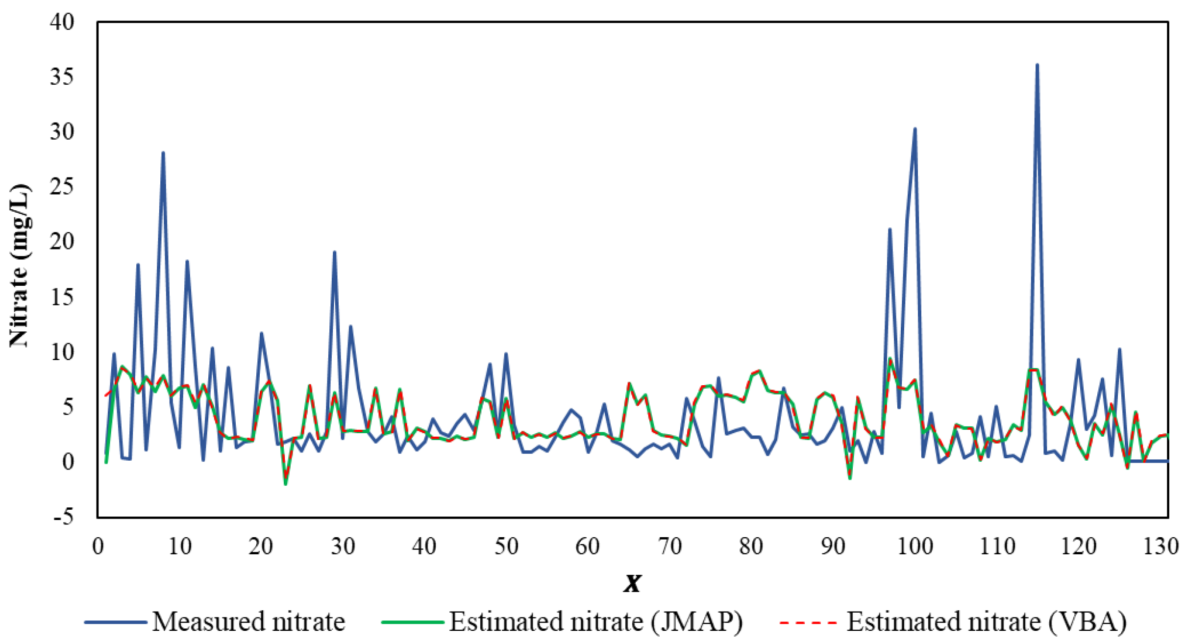
The results of JMAP and VBA regularizations for the DRASTICL parameter set are presented in Figure 2, illustrating the measured and inferred nitrate concentrations, respectively, C and C ^ . The inferred coefficients Ξ ^ and the inferred error bars for each parameter (i.e., Ξ Ξ ^ ) are presented in Table 1.
As evident in Figure 2, both JMAP and VBA methods exhibited similar performances in estimating nitrate concentrations. The remarkably small error bars ( σ ^ ), on the order of 10−9 to 10−11 (Table 1), indicate high precision in estimating coefficients. The ability to extract the standard deviations of the model coefficients demonstrates a key benefit of the Bayesian framework, allowing for extension to additional features of Bayesian inference such as uncertainty quantification.
The calculated correlation coefficient, R, for the JMAP and VBA methods, based on the raw nitrate data, as well as the index-based DRASTICL [13], are given in the second-last column of Table 2.
As shown in Table 2, both JMAP and VBA methods exhibited better performance in estimating nitrate concentrations compared to the traditional DRASTICL index-based method. The value of R increased from 0.2 for the DRASTICL index-based method, a weak positive correlation, to 0.4 for the JMAP and VBA methods, representing a moderate positive correlation [26,27,28].
Despite the improvements in the correlation coefficient, the R value is not strong in any of the Bayesian algorithms. To understand the low correlations of Table 2, the nitrate data were further analyzed. As presented in Figure 1, the nitrate data has a very different distribution compared with other input variables, characterized by sharp increases in concentration. To better understand the impact of this spiky nature of nitrate data on the goodness-of-fit, Fourier analysis [29] was applied to the nitrate data. First, the nitrate position data were transformed into the frequency domain using the Fast Fourier Transform (FFT) algorithm that computes the Discrete Fourier Transform (DFT) of a sequence, defined as:
x ( k ) = n = 0 N 1 x n . e 2 π i N k n
where x ( k ) is the k th frequency component of the DFT, x n is the input signal, N is the number of data points in the input signal, and i = 1 . A frequency filter was then applied to the frequency spectrum, to remove high-frequency spikes in nitrate concentrations. Various frequency thresholds of 0.05, 0.10, 0.20, 0.30, and 0.40 were applied to remove high-frequency components and eliminate the spikiness of the nitrate data. The filtered frequency ranges were then transformed back to the position domain applying the Inverse Fast Fourier Transform (IFFT):
x ( n ) = 1 N k = 0 N 1 x k . e 2 π i N k n
The reconstructed nitrate data were then incorporated into the JMAP and VBA algorithms. Results showed that the frequency threshold of 0.3 improved the correlations to a maximum Pearson correlation coefficient of 0.60 for both JMAP and VBA algorithms. These are given in the last column of Table 2. The DRASTICL index-based method does not incorporate the nitrate data, so its correlation is unchanged. These findings emphasize the irregular, spiked characteristics of nitrate data and their effect on correlation strength.

5. Discussion and Conclusions

This study demonstrates the application of inverse Bayesian methods, specifically the joint maximum a-posteriori (JMAP) and variational Bayesian approximation (VBA) algorithms, for groundwater vulnerability assessment (GVA) using spatial-series data. By focusing on nitrate concentrations in groundwater within the Burdekin Basin, Queensland, Australia, we highlight the advantages of the Bayesian approach over traditional index-based methods such as the DRASTICL method.
The application of inverse Bayesian methods represents a significant step forward in the field of groundwater vulnerability assessment. The Bayesian framework’s ability to provide detailed posterior probability distributions for model parameters allows for more precise parameter estimation and a better understanding of uncertainties. The adaptation of JMAP and VBA algorithms to spatial-series data marks a significant advancement, demonstrating their versatility and applicability beyond their traditional use with time-series data. Both JMAP and VBA algorithms outperform the traditional DRASTICL index-based method in terms of Pearson correlation coefficients (R).
The inferred coefficient vector Ξ ^ obtained from the Bayesian algorithms can be implemented as a groundwater vulnerability index throughout the study area using the geographical information system (GIS) software package [30]. This implementation allows the prediction of nitrate concentrations C ^ at locations where no direct observations are available. Consequently, the generation of a groundwater vulnerability map and its associated uncertainty map could provide valuable insights into environmental management or policy development in the region. This application will be explored elsewhere.
Despite the benefits of Bayesian methods over traditional approaches, the moderate correlations observed between measured and predicted nitrate concentrations ( C and C ^ ) indicate ongoing challenges in achieving a high goodness-of-fit. Future research should continue to refine these Bayesian methods, explore their application across different geographical contexts, and address the complexities of groundwater systems in more process-based models.

Author Contributions

Conceptualization, N.T. and R.K.N.; methodology, N.T. and R.K.N.; validation, N.T.; formal analysis, N.T.; data curation, N.T.; writing—original draft preparation, N.T.; writing—review and editing, R.K.N., M.K., and D.J.P.; visualization, N.T.; supervision, R.K.N., M.K. and D.J.P. All authors have read and agreed to the published version of the manuscript.

Funding

This research received no external funding.

Institutional Review Board Statement

Not applicable.

Informed Consent Statement

Not applicable.

Data Availability Statement

The dataset used in this study corresponds to the dataset used in [22]. This study represents the initial application of the Bayesian framework, while [22] provides a more detailed description of the dataset and related preprocessing steps. All data are available on request.

Conflicts of Interest

The authors declare no conflicts of interest.

References

  1. Brunton, S.L.; Proctor, J.L.; Kutz, J.N. Discovering governing equations from data by sparse identification of nonlinear dynamical systems. Proc. Natl. Acad. Sci. USA 2016, 113, 3932–3937. [Google Scholar] [CrossRef]
  2. Niven, R.K.; Mohammad-Djafari, A.; Cordier, L.; Abel, M.; Quade, M. Bayesian identification of dynamical systems. Proceedings 2020, 33, 33. [Google Scholar] [CrossRef]
  3. Mangan, N.M.; Kutz, J.N.; Brunton, S.L.; Proctor, J.L. Model selection for dynamical systems via sparse regression and information criteria. Proc. R. Soc. A Math. Phys. Eng. Sci. 2017, 473, 20170009. [Google Scholar] [CrossRef]
  4. Rudy, S.H.; Brunton, S.L.; Proctor, J.L.; Kutz, J.N. Data-driven discovery of partial differential equations. Sci. Adv. 2017, 3, e1602614. [Google Scholar] [CrossRef] [PubMed]
  5. Mojabi, P.; LoVetri, J. Overview and classification of some regularization techniques for the Gauss-Newton inversion method applied to inverse scattering problems. IEEE Trans. Antennas Propag. 2009, 57, 2658–2665. [Google Scholar] [CrossRef]
  6. Hào, D.N.; Lesnic, D. Heuristic regularization methods for numerical differentiation. Comput. Math. Appl. 2012, 63, 816–826. [Google Scholar] [CrossRef]
  7. Guckenheimer, J.; Holmes, P. Nonlinear Oscillations, Dynamical Systems, and Bifurcations of Vector Fields; Springer Science & Business Media: New York, NY, USA, 2013; Volume 42. [Google Scholar]
  8. Mohammad-Djafari, A.; Dumitru, M.J.D.S.P. Bayesian sparse solutions to linear inverse problems with non-stationary noise with Student-t priors. Digit. Signal Process. 2015, 47, 128–156. [Google Scholar] [CrossRef]
  9. National Research Council. Ground Water Vulnerability Assessment: Predicting Relative Contamination Potential Under Conditions of Uncertainty; The National Academies Press: Washington, DC, USA, 1993; 224p.
  10. Pavlis, M.; Cummins, E.; McDonnell, K. Groundwater vulnerability assessment of plant protection products: A review. Hum. Ecol. Risk Assess. 2010, 16, 621–650. [Google Scholar] [CrossRef]
  11. Taghavi, N.; Niven, R.K.; Paull, D.J.; Kramer, M. Groundwater vulnerability assessment: A review including new statistical and hybrid methods. Sci. Total Environ. 2022, 822, 153486. [Google Scholar] [CrossRef]
  12. Aller, L.; Truman, B.; Lehr, J.H. DRASTIC: A Standardized System for Evaluating Ground Water Pollution Potential Using Hydrogeologic Settings; Robert S. Kerr Environmental Research Laboratory, Office of Research And Development U.S. Environmental Protection Agency: Ada, OK, USA, 1985. [Google Scholar]
  13. Taghavi, N.; Niven, R.K.; Kramer, M.; Paull, D.J. Comparison of DRASTIC and DRASTICL groundwater vulnerability assessments of the Burdekin Basin, Queensland, Australia. Sci. Total Environ. 2023, 858, 159945. [Google Scholar] [CrossRef]
  14. Wu, X.; Marshall, L.; Sharma, A. The influence of data transformations in simulating Total Suspended Solids using Bayesian inference. Environ. Model. Softw. 2019, 121, 104493. [Google Scholar] [CrossRef]
  15. Fu, B.; Horsburgh, J.S.; Jakeman, A.J.; Gualtieri, C.; Arnold, T.; Marshall, L.; Green, T.R.; Quinn, N.W.T.; Volk, M.; Hunt, R.J.; et al. Modeling water quality in watersheds: From here to the next generation. Water Resour. Res. 2020, 56, e2020WR027721. [Google Scholar] [CrossRef] [PubMed]
  16. Marshall, L.; Nott, D.; Sharma, A. Towards dynamic catchment modelling: A Bayesian hierarchical mixtures of experts framework. Hydrol. Process. Int. J. 2007, 21, 847–861. [Google Scholar] [CrossRef]
  17. Zhao, Y.; Sharma, A.; Sivakumar, B.; Marshall, L.; Wang, P.; Jiang, J. A Bayesian method for multi-pollution source water quality model and seasonal water quality management in river segments. J. Environ. Model. Softw. 2014, 57, 216–226. [Google Scholar] [CrossRef]
  18. Tang, Y.; Marshall, L.; Sharma, A.; Ajami, H. A Bayesian alternative for multi-objective ecohydrological model specification. J. Hydrol. 2018, 556, 25–38. [Google Scholar] [CrossRef]
  19. Zeng, L.; Li, J. A Bayesian belief network approach for mapping water conservation ecosystem service optimization region. J. Geogr. Sci. 2019, 29, 1021–1038. [Google Scholar] [CrossRef]
  20. Oliveira, R.; Scalzo, R.; Kohn, R.; Cripps, S.; Hardman, K.; Close, J.; Taghavi, N.; Lemckert, C. Bayesian optimization with informative parametric models via sequential Monte Carlo. Data-Centric Eng. 2022, 3, e5. [Google Scholar] [CrossRef]
  21. Cahill, N.; Croke, J.; Campbell, M.; Hughes, K.; Vitkovsky, J.; Kilgallen, J.E.; Parnell, A. A Bayesian time series model for reconstructing hydroclimate from multiple proxies. Environmetrics 2023, 34, e2786. [Google Scholar] [CrossRef]
  22. Taghavi, N.; Niven, R.K.; Kramer, M.; Paull, D.J. Enhancing groundwater vulnerability assessment through Bayesian inference. J. Hydrol. 2025, 653, 132781. [Google Scholar] [CrossRef]
  23. Bayes, T. LII. An essay towards solving a problem in the doctrine of chances. By the late Rev. Mr. Bayes, F. R. S. communicated by Mr. Price, in a letter to John Canton, A. M. F. R. S. Philos. Trans. R. Soc. Lond. 1763, 53, 370–418. [Google Scholar] [CrossRef]
  24. Mahalanobis, P.C. Reprint of: Mahalanobis, P.C. (1936) "On the Generalised Distance in Statistics.". Sankhya A 2019, 80, 1–7. [Google Scholar] [CrossRef]
  25. MATLAB, version: 9.8.0.1323502 (R2020a); The MathWorks, Inc.: Natick, MA, USA, 2020.
  26. Dancey, C.; Reidy, J.; Rowe, R. Statistics for the Health Sciences: A Non-Mathematical Introduction; Sage Publications: Thousand Oaks, CA, USA, 2012. [Google Scholar]
  27. Akoglu, H. User’s guide to correlation coefficients. Turk. J. Emerg. Med. 2018, 18, 91–93. [Google Scholar] [CrossRef] [PubMed]
  28. Turney, S. Pearson Correlation Coefficient (r)|Guide & Examples. 2023. Available online: https://www.scribbr.com/statistics/pearson-correlation-coefficient/ (accessed on 27 June 2023).
  29. Bochner, S.; Chandrasekharan, K. Fourier Transforms; Princeton University Press: Princeton, NJ, USA, 1949. [Google Scholar]
  30. ESRI. ArcGIS Desktop: Release 10.6; Environmental Systems Research Institute: Redlands, CA, USA, 2018. [Google Scholar]
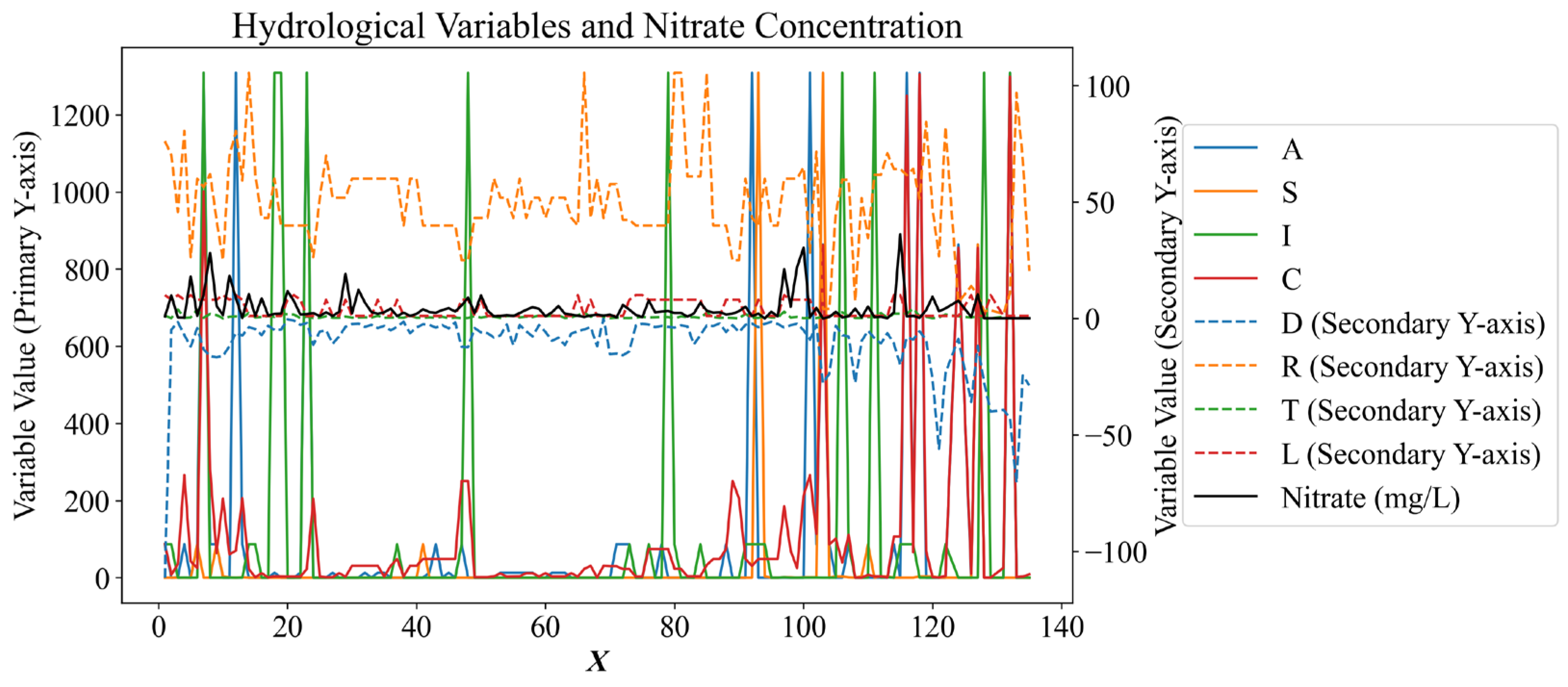
Figure 1. Independent parameters used in the analysis as functions of spatial index X (units are disregarded).
Psf 12 00014 g001
Figure 2. Comparison of measured and predicted nitrate values using JMAP and VBA regularization methods versus spatial series X .
Psf 12 00014 g002
Table 1. Inferred coefficients Ξ ^ and the inferred standard deviations for each parameter.
No.Parameter Ξ ^ σ ^
JMAPVBAJMAPVBA
1D2.33 × 10−22.24 × 10−21.206 × 10−104.632 × 10⁻¹¹
2R3.47× 10−23.48 × 10−25.948 × 10−116.684 × 10⁻¹²
3A−2.78 × 10⁻³−2.54 × 10−34.709 × 10−111.262 × 10⁻¹¹
4S−2.13 × 10⁻⁵−1.93 × 10−63.177 × 10−93.163 × 10⁻¹⁰
5T4.25 × 10−13.61 × 10−15.156 × 10−93.271 × 10⁻⁹
6I−4.80 × 10⁻⁴−3.98 × 10−45.154 × 10−124.155 × 10⁻¹²
7C4.63 × 10−34.59 × 10−31.891 × 10−112.869 × 10⁻¹²
8L5.33 × 10−15.43 × 10−17.696 × 10−105.162 × 10⁻¹⁰
Table 2. Pearson correlation coefficient for different methods.
No.MethodR
(Unfiltered Data)
R
(Fourier Transform Filter)
1JMAP0.40.6
2VBA0.40.6
3Index-based DRASTICL [13]0.2
Disclaimer/Publisher’s Note: The statements, opinions and data contained in all publications are solely those of the individual author(s) and contributor(s) and not of MDPI and/or the editor(s). MDPI and/or the editor(s) disclaim responsibility for any injury to people or property resulting from any ideas, methods, instructions or products referred to in the content.