Detection of Net Blotch Disease of Barley Using UAV-Based RGB and Multispectral Imagery at Plot Scale ^†

Abstract

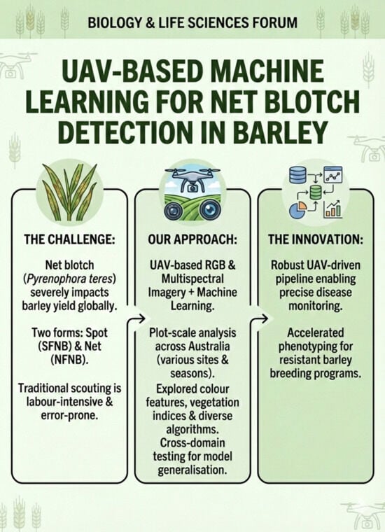
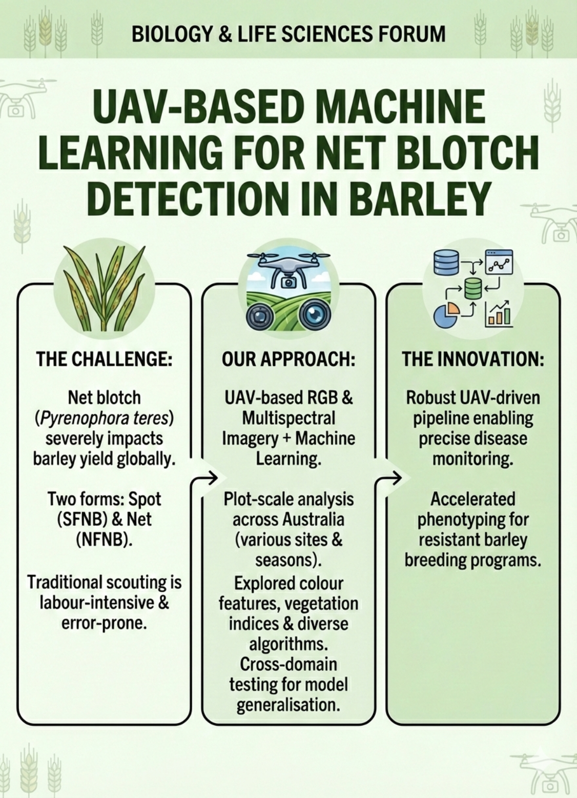
Net blotch, caused by Pyrenophora teres, is a major barley disease that occurs in two forms, spot form net blotch (SFNB) and net form net blotch (NFNB), reducing grain yield and quality worldwide. Accurate detection is critical for disease management and breeding resistant cultivars; however, traditional disease scoring is labour-intensive and error-prone. This study evaluates the use of UAV-based red–green–blue (RGB) and multispectral imagery, combined with machine learning, for determining net blotch infection levels at the plot scale across multiple sites and seasons in Australia. Various colour features, vegetation indices, and algorithms were tested, including a cross-domain testing for model generalisation. We propose a robust UAV-driven pipeline enabling precise disease monitoring and phenotyping in barley breeding programs.

1. Introduction

Barley (Hordeum vulgare L.) is one of the world’s most vital cereal crops [1]. Among the main threats to barley production, net blotch, caused by the fungal pathogen Pyrenophora teres, is especially damaging, causing yield reductions of 10–40% worldwide [2]. In Australia, it is the most harmful foliar disease of barley, responsible for around 42% of yearly losses, which amounts to about AUD 125 million [2]. Net blotch appears in two forms: net form net blotch (NFNB), characterised by elongated, net-like dark-brown lesions, and spot form net blotch (SFNB), which features elliptical dark-brown lesions. The pathogen survives on stubble and can also be seed-borne, making management difficult.

Developing resistant cultivars and effective fungicide strategies is critical for sustainable barley production. However, breeding programs and disease management rely on rapid and accurate phenotyping, which remains a major bottleneck. Current field phenotyping is labour-intensive, subjective, and dependent on expert assessment [3]. Recent advances in optical sensing, sensor platforms, and artificial intelligence (AI) offer transformative opportunities for high-throughput, non-destructive, and cost-effective phenotyping. Commonly used sensors include RGB, multispectral, and hyperspectral cameras, which can be mounted on uncrewed aerial vehicles (UAVs) for flexible, low-altitude imaging. AI techniques, including classical machine learning and deep learning architectures such as ResNet, DenseNet, and transformers, have shown promise in detecting visible and latent disease symptoms at leaf, canopy, and plot scales [4].

This study examines the potential of combining UAV-based RGB and multispectral imaging with machine learning to estimate net blotch severity at the plot scale. The proposed approach aims to deliver a high-throughput, accurate, and affordable phenotyping solution suitable for breeding programs and accessible to users with minimal pathology expertise.

2. Materials and Methods

2.1. Field Trials Preparation

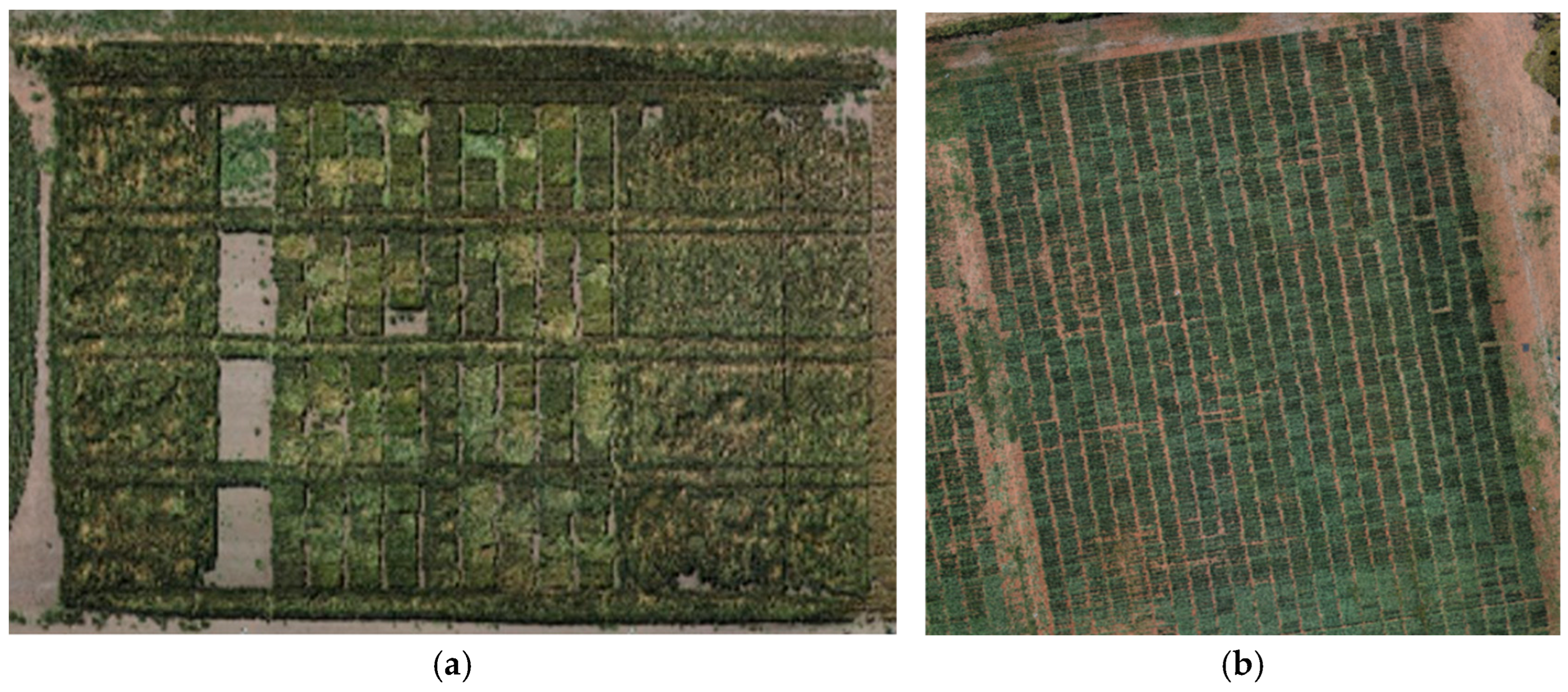
Two field trials were conducted in Horsham, Victoria, and Turretfield, South Australia in 2023 and 2024 (Figure A1). Barley varieties of varying net blotch resistance were sown with the plot size of about 1 m × 2 m or 2 m × 2 m. Spreader lines were interspaced in the middle of the trial to promote fungal infection. The Horsham trial had 128 plots in 2023 and 144 plots in 2024. The Turretfield trial dataset included 2791 plots in 2023 and 4464 plots in 2024.

2.2. Data Collection

When the disease symptoms appeared, experienced pathologists scored each plot visually from 0 to 100%. The scores of SFNB and NFNB were recorded separately, and the sum of SFNB and NFNB scores was used as the overall disease score. Immediately after scoring, a DJI Matrice 300 (SZ DJI Technology Co., Ltd., Shenzheng, China) equipped with the Zenmuse P1 RGB camera and MicaSense RedEdge multispectral camera (AgEagle Aerial Systems Inc., Wichita, KS, USA) were flown at 12 m height to image the plots, giving a ground resolution of about 1.5 mm/pixel for RGB images and 7.5 mm/pixel for the five-band multispectral images, respectively. The five channels of the multispectral images were blue (475 nm centre), green (560 nm centre), red (668 nm centre), red edge (717 nm centre) and near-infrared (842 nm centre).

2.3. Data Pre-Processing

Data pre-processing involved three steps. In the first step, the georeferenced images were processed to generate a seamless mosaic using a Structure-from-Motion (SfM) algorithm implemented in the Agisoft Metashape software 2.3.0 (Agisoft Metashape, Saint Petersburg, Russia). This approach uses visible features across the overlapping RGB and multispectral images for accurate construction of spatially consistent orthomosaic for further quantitative analysis. The second step was georeferencing, which linked each plot polygon to its ground-truth disease score using the ArcGIS Pro 3.6.2 software (Environmental Systems Research Institute, Inc., Redlands, CA, USA). The third step was removing non-plant pixels, including soil, shadows, and over-saturated pixels such as highly reflective spots on leaves, using colour-based thresholding. In the RGB images, we first converted RGB orthomosaics into the hue-saturation-value (HSV) colour space and extracted the masks of barley plants using the images of hue, saturation and value in Equations (1)–(4), where $m_{ip}$, $m_s$, $m_o$ and $m_{fp}$ represents the initial mask images of barley plants, shadows, over-saturated pixels and the final plant mask after removing shadows and over-saturated pixels, respectively. h stands for the hue images, $h_{pl}$ (default 75) for the lower threshold of plants in the hue images, $h_{ph}$ (default 30) for the upper threshold of plants in the hue images, s for the images of saturation, v for the images of value, $s_s$ (default 0.2) for the threshold of shadows in the images of saturation, $v_s$ (default 0.2) for the threshold of shadows in the images of value and $v_o$ (default 0.95) for the threshold of over-saturated pixels in the images of value.

$$m_{ip}=\left(h\ge {\displaystyle \frac{120-h_{pl}}{360}}\right)\&\left(h\ge {\displaystyle \frac{120+h_{ph}}{360}}\right)$$

(1)

$$m_s=s<s_s\&v<v_s$$

(2)

$$m_o=v>v_o$$

(3)

$$m_{fp}=m_{ip}\&(~m_s)\&{(~m}_o)$$

(4)

Similarly, in the multispectral images, we first converted the multispectral images into the hyper-hue-saturation-intensity (HHSI) colour space [5] and then used Equations (5)–(8) to extract the masks of barley plants. In Equations (5)–(8), $m_{ip}$, $m_s$, $m_o$ and $m_{fp}$ represents the initial mask images of barley plants, shadows, over-saturated pixels and the final plant mask. ${hh}_2$ stands for the mages of the second dimension of hyper-hue, which is a multispectral version of hue; ${hh}_{2p}$ (default −0.2) for the threshold of plants in ${hh}_2$; $i$ for the images of intensity; $i_s$ (default 0.03) for the threshold of shadows in the images of intensity; and $i_o$ (default 0.85) for the threshold of over-saturated pixels in the images of $i$.

$$m_{ip}={hh}_2>{hh}_{2p}$$

(5)

$$m_s=i<i_s$$

(6)

$$m_o=i>i_o$$

(7)

$$m_{fp}=m_{ip}\&(~m_s)\&{(~m}_o)$$

(8)

2.4. Statistical Analysis of Disease Score

The histograms of disease scores were plotted to observe the distributions of the scores for the respective trial sites and years. Further, box whisker plots of disease scores for replicated check varieties were produced to observe the disease resistance levels of the barley varieties.

2.5. Plot Feature Extraction

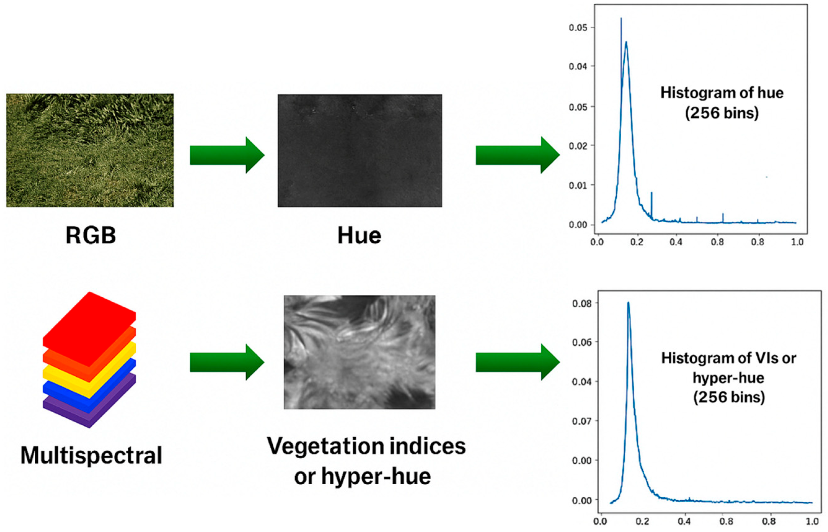
From each plot, we extracted 36 different features, which are based on the histograms of colour or spectral properties of plants. The RGB orthomosaics were first converted from the RGB colour space to the HSV colour space, and then the histogram of hue values was extracted as a plot feature, which can capture the yellowing or browning colours of disease symptoms (Top row of Figure 1). In the multispectral images, we extracted the histograms of 11 common vegetation indices. Besides that, we extracted the histogram of hyper-hue from the HHSI space (

Table A1. Plot features (The formulas are in Python format. The value of eps was set to 10⁻¹⁰).

Feature	Description
B1	Hue in HSI colour space. It represents the pure colour.
B2	NDVI (Normalised Difference Vegetation Index): Measures vegetation health using NIR and Red. NDVI = (nir − red)/(nir + red + eps)
B3	GNDVI (Green NDVI): Similar to NDVI but uses Green instead of Red; sensitive to chlorophyll. GNDVI = (nir − green)/(nir + green + eps)
B4	NDRE (Normalised Difference Red Edge Index): Detects stress in vegetation using NIR and Red Edge. NDRE = (nir − red_edge)/(nir + red_edge + eps)
B5	TVI (Transformed Vegetation Index): Enhances NDVI contrast using square root transformation. TVI = np.sqrt((nir − red)/(nir + red + eps) + 0.5)
B6	GRVI (Green-Red Vegetation Index): Simple ratio of Green to Red; indicates vegetation vigour. GRVI = green/(red + eps)
B7	NDGI (Normalised Difference Green Index): Highlights green vegetation using Green and Red. NDGI = (green − red)/(green + red + eps)
B8	MSAVI (Modified Soil Adjusted Vegetation Index): Designed to further reduce the influence of bare soil without requiring you to choose a soil adjustment factor (L)) msavi = (2 × nir + 1 − np.sqrt((2 × nir + 1) ** 2 − 8 × (nir − red)))/2
B9	Clgreen (Chlorophyll index): Estimates chlorophyll content in leaves. useful for precision agriculture and stress detection. Clgreen = nir/(green + eps) − 1
B10	Hyper-hue-3D in HHSI space: It was transformed from the hypercube composed of green, red, red-edge and near-infrared bands. It reduces the effects of shadowing and specular effects in hyperspectral images [5].
B11	EVI (Enhanced Vegetation Index): Improves sensitivity in high biomass regions; reduces atmospheric effects. EVI = 2.5 × (nir − red)/(nir + 6 × red − 7.5 × blue + 1 + eps)
B12	VARI (Visible Atmospherically Resistant Index): Uses visible bands; robust to atmospheric noise. VARI = (green − red)/(green + red − blue + eps)
B13	Hyper-hue-4D in HHSI space: It was transformed from the hypercube composed of blue green, red, red-edge and near-infrared bands. It reduces the effects of shadowing and specular effects in hyperspectral images [5].
S1	Hue + NDVI
S2	Hue + GNDVI
S3	Hue + NDRE
S4	Hue + TVI
S5	Hue + GRVI
S6	Hue + NDGI
S7	Hue + MSAVI
S8	Hue + Clgreen
S9	Hue + Hyper-hue-3D
S10	Hue + EVI
S11	Hue + VARI
S12	Hue + Hyp-hue-4D
E1	Hue + NDVI + GNDVI
E2	Hue + NDVI + GNDVI + NDRE
E3	Hue + NDVI + GNDVI + NDRE + TVI
E4	Hue + NDVI + GNDVI + NDRE + TVI + GRVI
E5	Hue + NDVI + GNDVI + NDRE + TVI + GRVI + NDGI
E6	Hue + NDVI + GNDVI + NDRE + TVI + GRVI + NDGI + MSAVI
E7	Hue + NDVI + GNDVI + NDRE + TVI + GRVI + NDGI + MSAVI + Clgreen
E8	Hue + NDVI + GNDVI + NDRE + TVI + GRVI + NDGI + MSAVI + Clgreen + Hyp-hue-3D
E9	Hue + NDVI + GNDVI + NDRE + TVI + GRVI + NDGI + MSAVI + Clgreen + Hyp-hue-3D + EVI
E10	Hue + NDVI + GNDVI + NDRE + TVI + GRVI + NDGI + MSAVI + Clgreen + Hyp-hue-3D + EVI + VARI
E11	Hue + NDVI + GNDVI + NDRE + TVI + GRVI + NDGI + MSAVI + Clgreen + Hyp-hue-3D + EVI + VARI + Hyp-hue-4D

and the bottom row of Figure 1). Finally, we created various combinations of the histograms of the vegetation indices and hyper-hue to generate additional plot features.

2.6. Training and Validating Classification Models in Individual Datasets

Initial experiments involved developing regression models to predict exact disease scores and multi-class models to categorise infection levels as low, medium or high. However, these models exhibited poor performance, likely due to constraints in imaging angle, skewed data distribution and potential bias in ground-truth disease scores. Consequently, a binary classification approach was adopted to distinguish between high and low infection levels.

To establish meaningful disease thresholds for binary classification, we utilised the Horsfall–Barratt (H–B) scale, a standardised semi-quantitative system widely used for estimating plant disease severity [6]. The H–B scale divides disease intensity (0–100%) into 12 unequal, logarithmically spaced intervals designed to reflect human perception of the diseased area. Specifically, H–B rating 4 corresponds to 6–12% severity, rating 5 to 12–25%, and rating 6 to 25–50%. Given that the majority of observed disease scores in this study fell below 50%, we evaluated four disease-score thresholds, $t_d$, at 6%, 12%, 25%, and 50%.

For each dataset, categorised by field and year, four classical machine learning algorithms were implemented and validated: Support Vector Machine (SVM), Random Forest, Neural Networks and Naïve Bayes. Because the class sizes were highly imbalanced, with far more healthy samples than infected samples, model performances were evaluated using accuracy, precision, recall, F1-score, Cohen’s Kappa Coefficient (Kappa) and area under the curve of precision-recall (PR-AUC). Accuracy measures the overall proportion of correct predictions but can be misleading under class imbalance. Precision reflects the proportion of predicted positives that are true positives, while recall measures the proportion of actual positives correctly identified. The F1 score provides a balanced summary by combining precision and recall. Cohen’s Kappa accounts for agreement occurring by chance, offering a more robust measure of classifier reliability on imbalanced datasets. PR-AUC evaluates the trade-off between precision and recall across thresholds and is particularly informative when the positive class is rare. To ensure robustness and mitigate overfitting, we employed ten-fold cross-validation for each dataset.

2.7. Cross-Domain Testing

Most machine learning models are predicated on the fundamental assumption that training and testing data are independent and identically distributed (IID). When this assumption is violated, a phenomenon known as domain shift, model performance typically degrades significantly as the learned patterns fail to generalise to the new distribution. In this study, we conducted cross-domain evaluations to assess the generalisability of models trained on a single dataset when applied to datasets collected across different years and geographic fields.

2.8. Classification Model Optimisation

The default classifier uses a fixed decision threshold of $t_m=0.5$, which is not robust across different domains or disease-score thresholds. To enhance robustness, we propose a method that dynamically selects an optimised classification threshold that adapts to the domain, disease-score threshold, and plot features. During training, the method generates a precision–recall curve and identifies the threshold that yields the maximum F1-score on the training data. During validation and testing, the model then applies this adaptive threshold instead of the default value.

3. Results

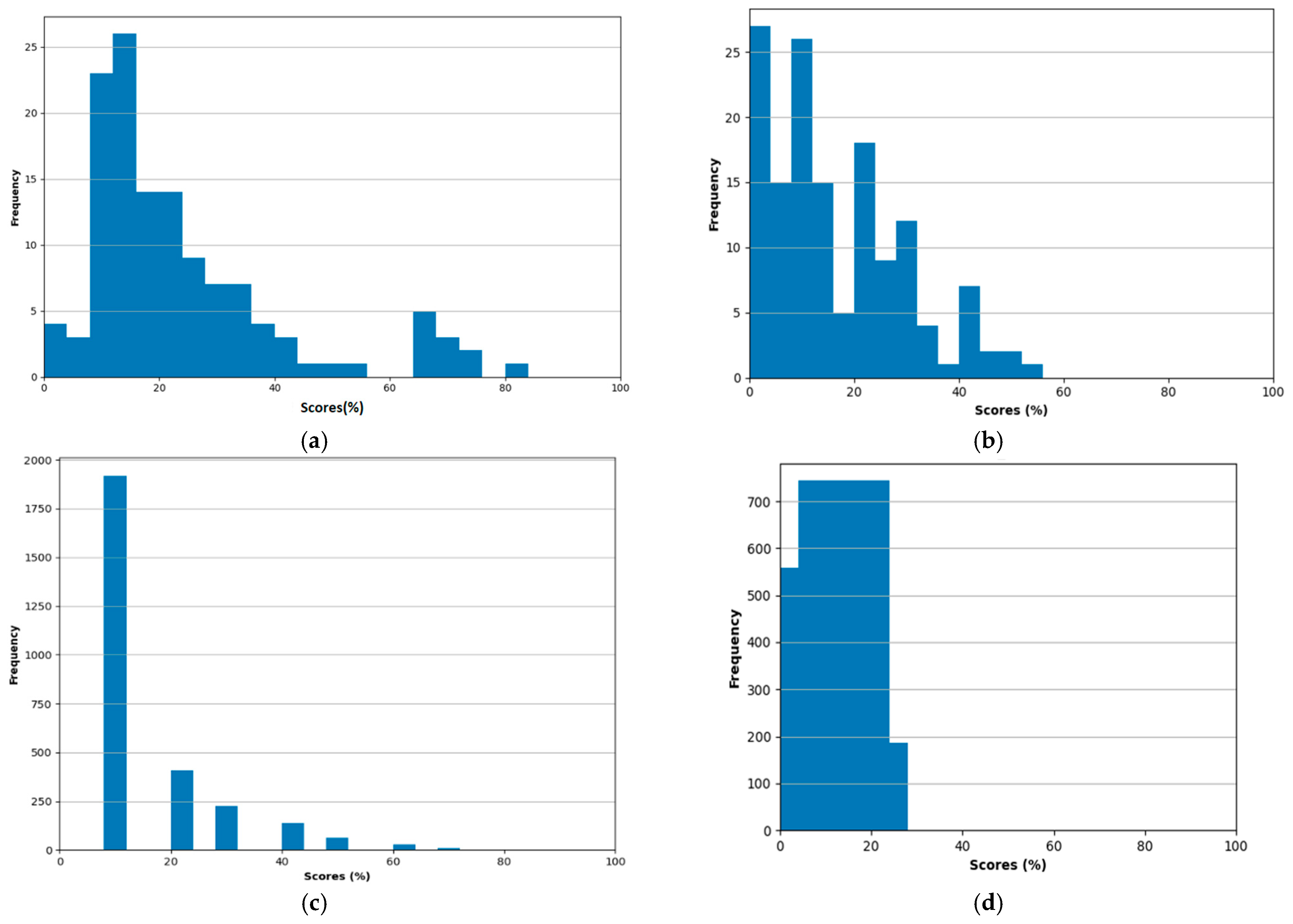
Figure 2 illustrates the distribution of disease scores across the four datasets. Most datasets exhibited a significant right-skew, with the majority of observations concentrated in the low-severity range. Notably, the Turretfield 2024 field trial was severely impacted by drought, which hindered disease progression; consequently, almost no plots exceeded 30% infection. Due to this lack of variance and insufficient infection levels, this dataset was deemed unsuitable for robust modelling and was excluded from further analysis.

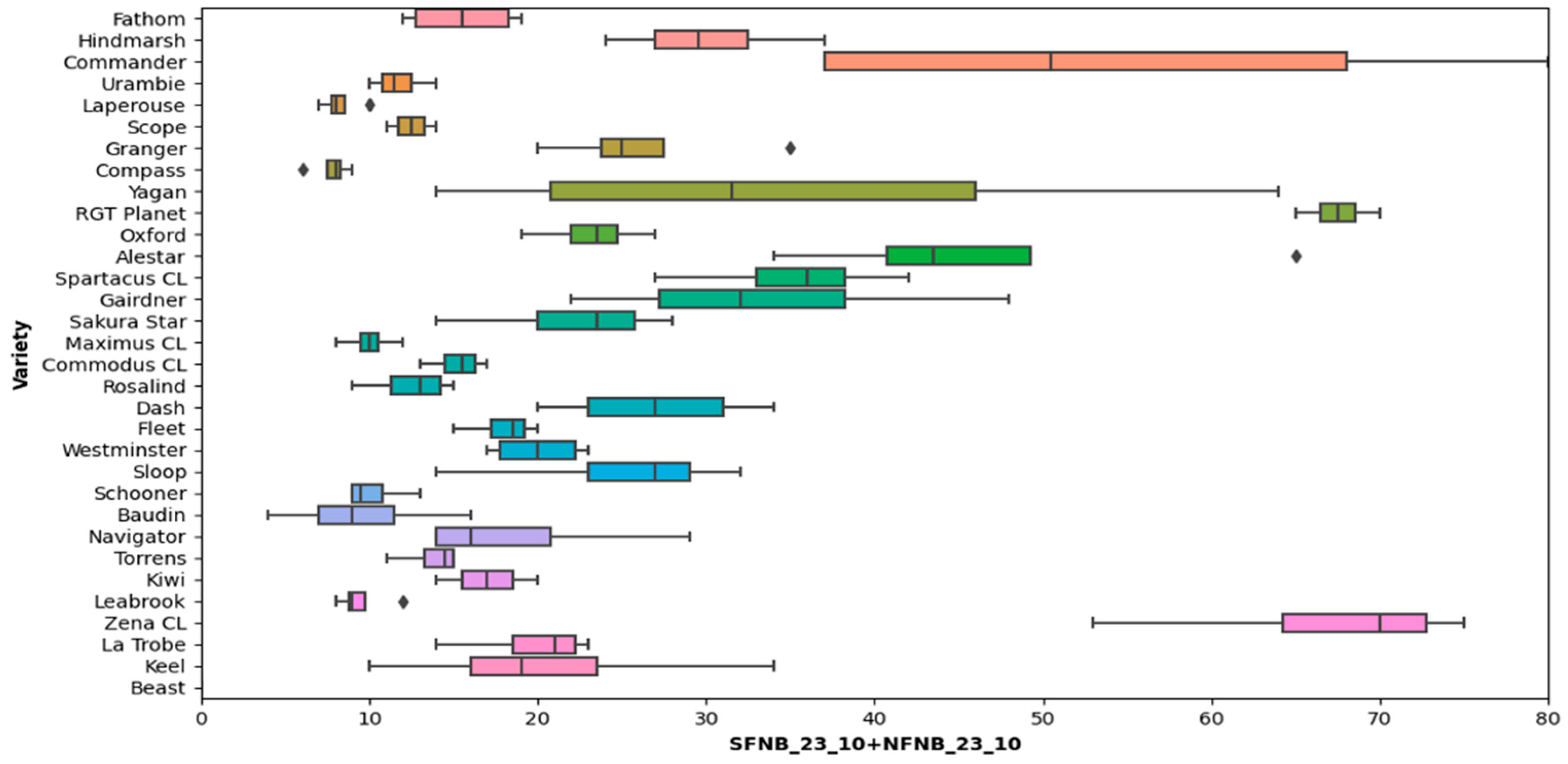
As shown in Figure A2, there was a marked difference in disease response among barley varieties. Highly resistant varieties, such as Leabrook, consistently maintained infection levels below 10%. In contrast, susceptible varieties like RGT Planet reached an average disease severity of 70%, highlighting the broad phenotypic range present in the remaining datasets.

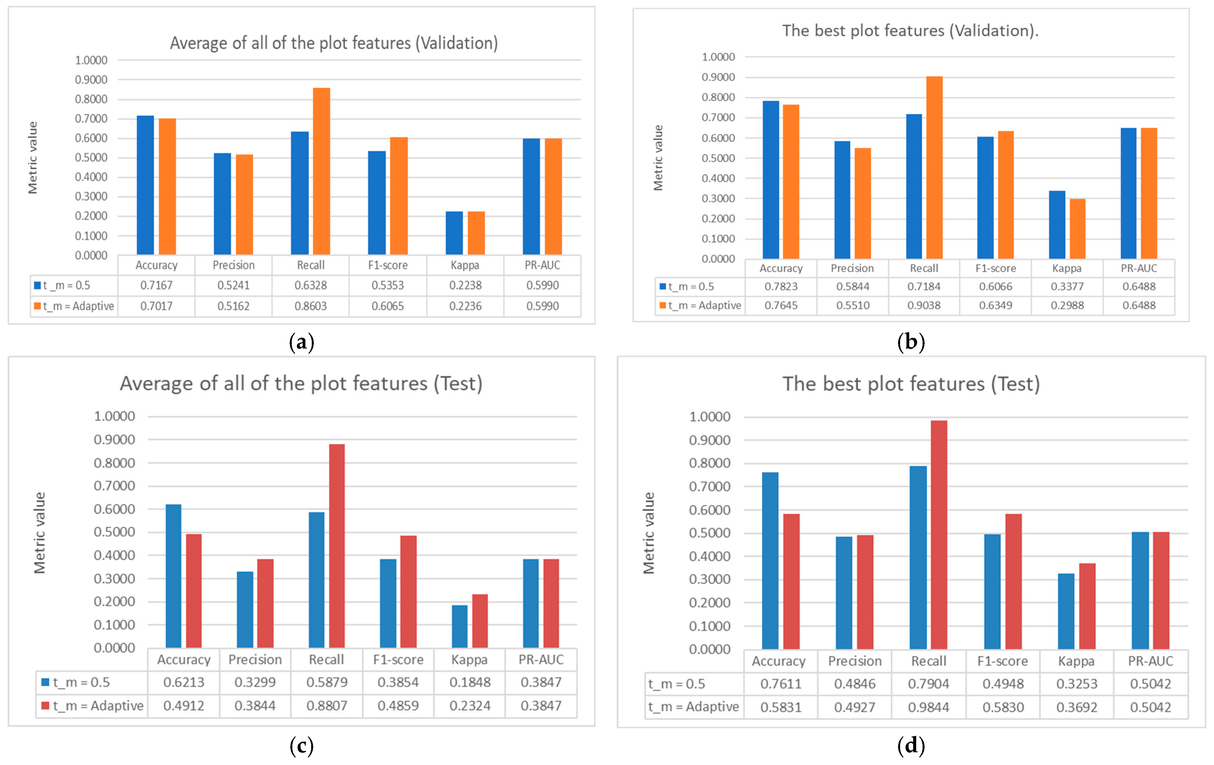
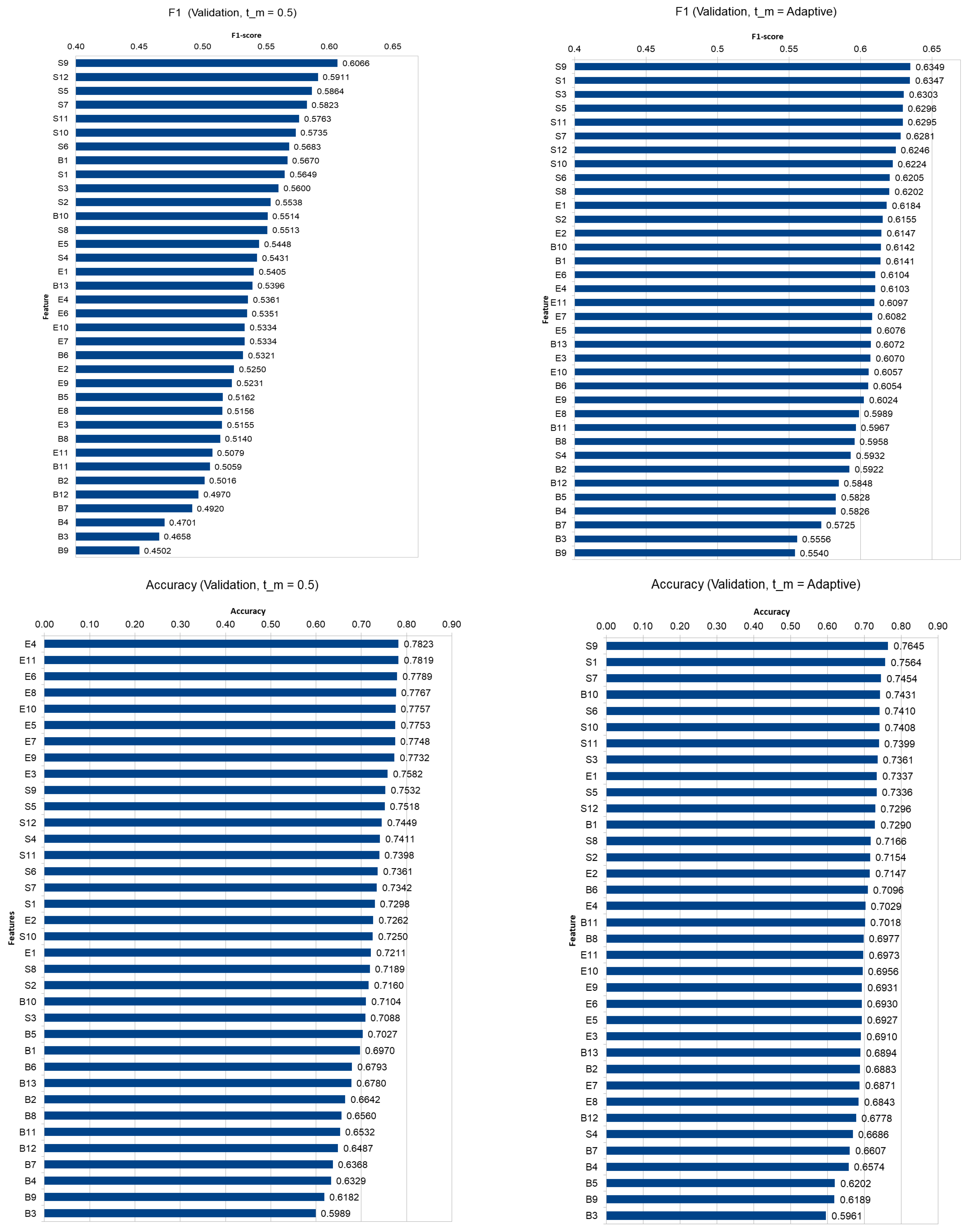
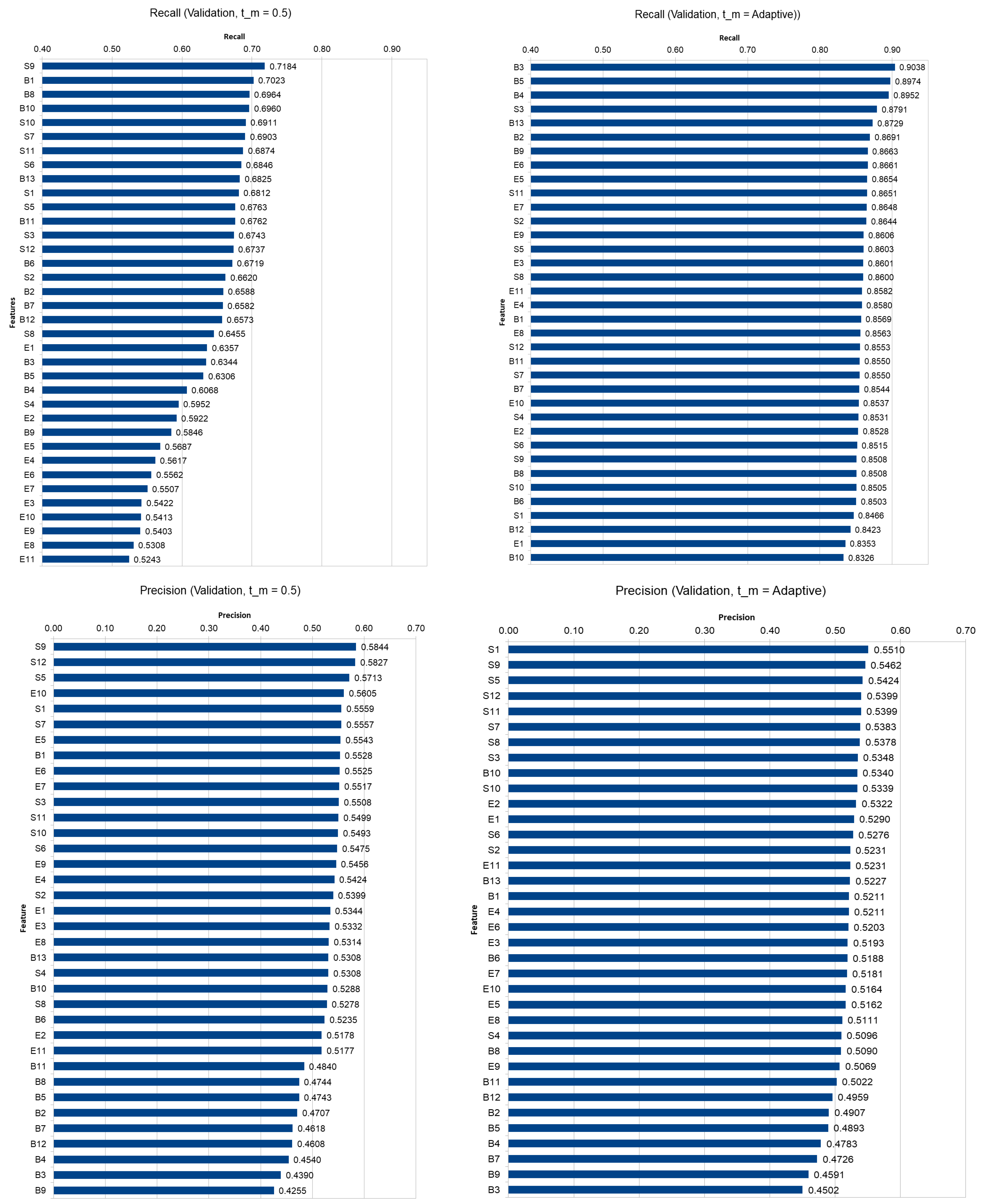
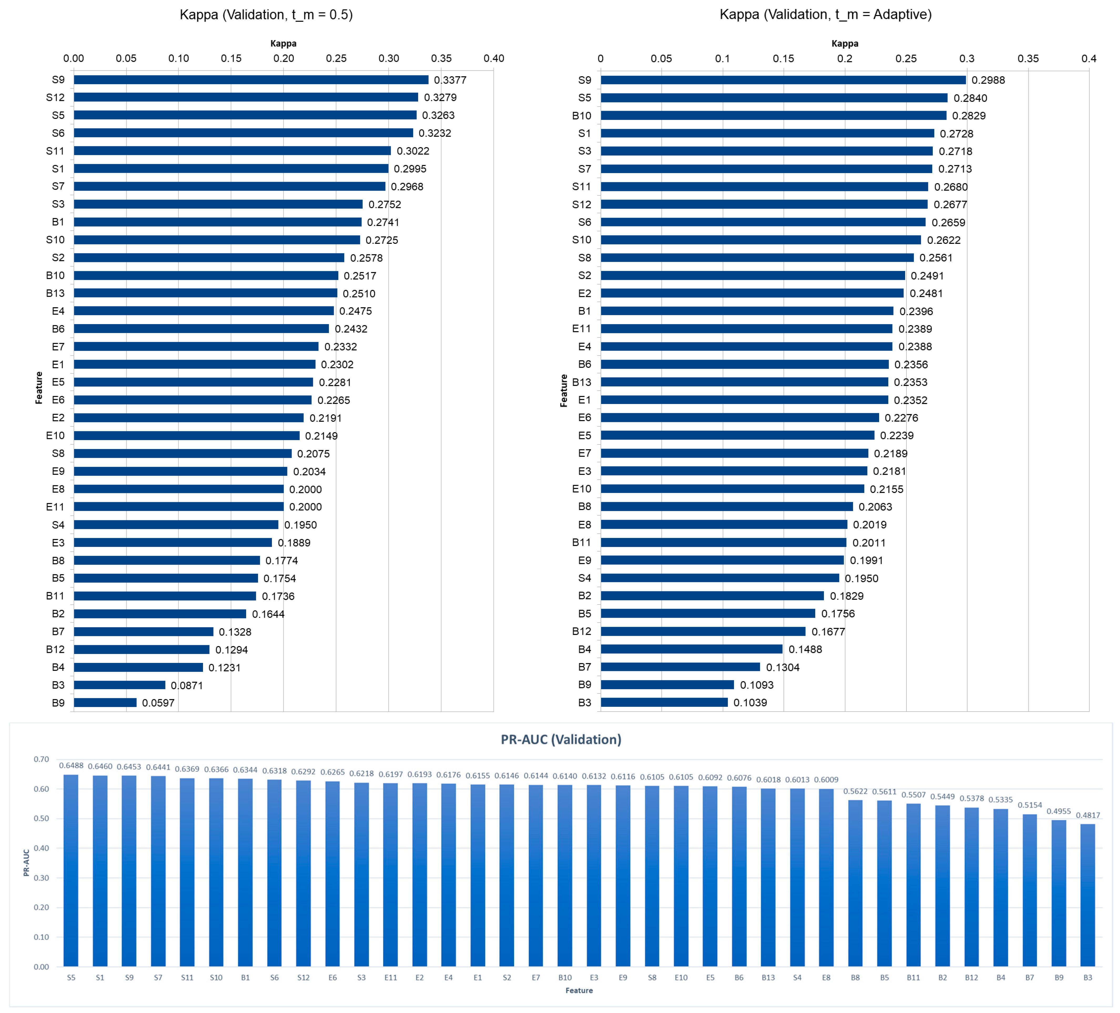
The cross-validation results are summarised in Figure 3a,b. Panel (a) shows the performance metrics averaged across all plot features, domains, and disease-score thresholds, while panel (b) presents the performance obtained using the best-performing plot features after averaging across domains and disease-score thresholds. Using the default classification threshold $t_m=0.5$, the averaged F1-score, Kappa, and PR-AUC across all plot features are 0.5353, 0.2238, and 0.5990, respectively, indicating moderate classification performance. When focusing on the best plot features, these values increase to 0.6066, 0.3377, and 0.6488 respectively, showing a meaningful improvement.

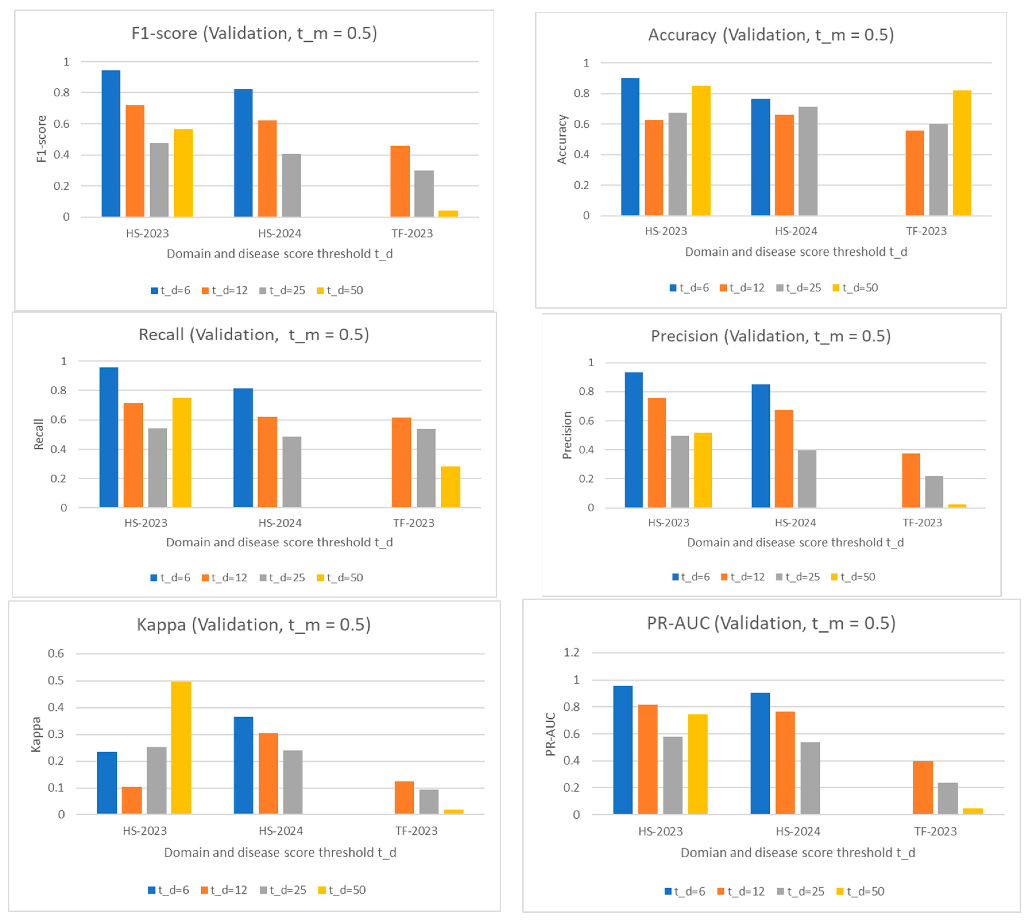
We found that different domains and disease-score thresholds have a substantial impact on classification performance (Figure A3). To improve robustness, we introduced a method that dynamically selects an optimised decision threshold $t_m$ that adapts to the domain, disease-score threshold, and plot features. With the adaptive $t_m$, the F1-score increased from 0.5653 to 0.6065 when averaging across all plot features (Figure 3a), and from 0.6066 to 0.6349 when using the best plot features (Figure 3b). This approximate 5% relative improvement in F1-score is notable, particularly in settings with noisy labels, class imbalance, and complex decision boundaries.

Compared with the cross-validation results, both models exhibited performance degradation in the cross-domain tests. When averaging across all plot features and using the default threshold $t_m$, the F1-score dropped from 0.5353 to 0.3854, an approximate 28% relative decrease (Figure 3c). In contrast, when applying the adaptive threshold $t_m$, the F1-score decreased from 0.6065 to 0.4859, corresponding to a 20% relative drop (Figure 3c). This smaller decline indicates that the adaptive thresholding strategy provides improved robustness under cross-domain conditions.

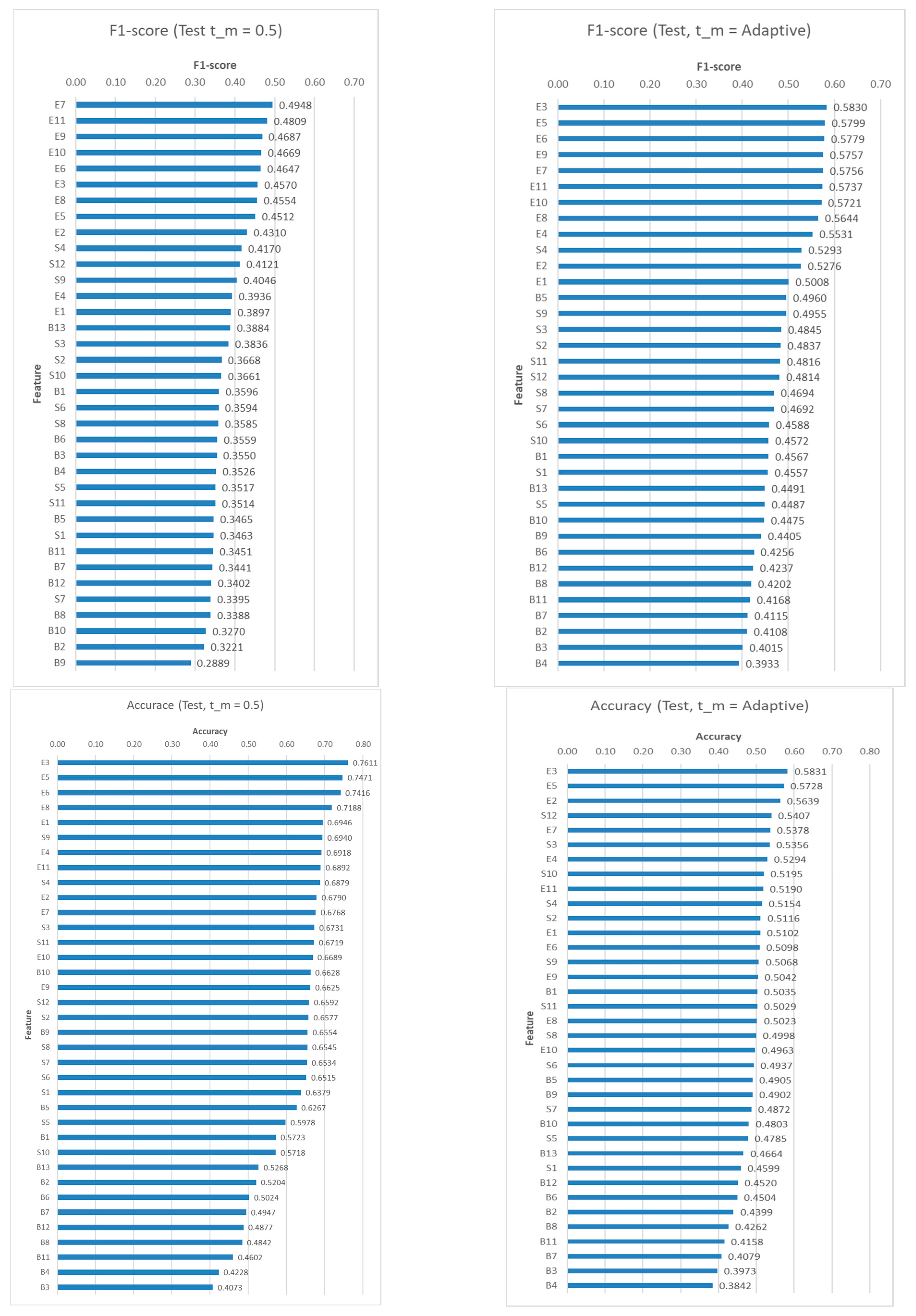
The benefit of the adaptive threshold becomes even more apparent when using the best plot features. With the default threshold, the F1-score dropped from 0.6066 in cross-validation to 0.4948 in cross-domain testing, an 18% decrease (Figure 3d). In contrast, with adaptive thresholds, the drop was much smaller, from 0.6349 to 0.5830 (Figure 3d), only 8%, representing a substantial improvement in robustness and generalisation performance.

4. Discussion

4.1. Platform and Sensors

While recent literature primarily focuses on leaf-scale plant disease detection under controlled environments using handheld sensors, there is an urgent, yet technically challenging, need for automated detection at the plot scale within field environments. This study investigates the feasibility of utilising UAV platforms equipped with RGB and multispectral sensors to estimate the severity of net blotch at the plot scale. Our findings demonstrate significant potential for developing high-throughput, accurate, and cost-effective phenotyping solutions tailored for breeding programs and accessible to users with limited pathological expertise.

Pathologists assess disease severity by examining both the upper and lower canopy layers. Plants with severe infections typically show visible symptoms on the first and the second flag leaves in the upper canopies. In contrast, at earlier stages of infection or lower levels of infection, symptoms often appear first on the lower leaves, which are important for distinguishing differences in disease tolerance among genotypes. However, the UAV-based imaging system captured only top-down views, limiting observations to the upper canopy layers and missing symptoms on lower leaves. This limitation reduces the ability to detect early or low-level infections accurately and helps explain the high number of false-negative errors observed in the model.

4.2. Data Distribution and Ground Truth

Due to the nature of disease progression in the field, most datasets exhibited a significant right skew, with observations concentrated in the low-severity range. Furthermore, we identified inconsistencies in scoring protocols between trials. For instance, pathologists in Horsham utilised a continuous scale of 0% to 100% with 1% increments, whereas those at the Turretfield site utilised a discrete 10% interval (refer to Figure 2). These distribution imbalances and inconsistent ground-truth labelling pose significant challenges for machine learning. Because of the skewed data distribution, there were far more negative instances than positive ones. As a result, the trained models tended to classify positive samples as negative, leading to a high false-negative rate. We also found that data distribution had a greater influence on model performance than dataset size. For example, the Horsham trials in 2023 and 2024 contained only 128 and 144 plots, respectively; however, due to their relatively more balanced data distributions (Figure 2), models trained on these datasets achieved substantially better performance than those trained on the Turretfield trials from 2023 and 2024 (Figure A3), which contained 2791 and 4464 plots, respectively. This highlights that simply increasing the amount of data does not guarantee improved performance when the underlying distribution is highly skewed.

To address these challenges, we first reformulated the continuous severity-estimation task into a more robust binary classification problem that discriminates between low- and high-level infections, a more practical framework for rapid field screening. We then modified the loss function to penalise false-negative errors more heavily, thereby reducing the risk of missing severe infections. In addition, we introduced an adaptive decision-thresholding strategy to enhance F1-score under varying data distributions. Together, these approaches substantially reduced false negative rate and therefore improved overall model performance.

4.3. Feature Engineering at the Plot Scale

While deep learning is currently a dominant research trend in data analysis, the limited size of our datasets favoured the use of classical machine learning models. In this context, the engineering of discriminative plot-level features is critical for model performance. We generated feature sets based on histograms of hue, hyper-hue, and various VIs to capture variations in plant colour, vigour, and photosynthetic activity.

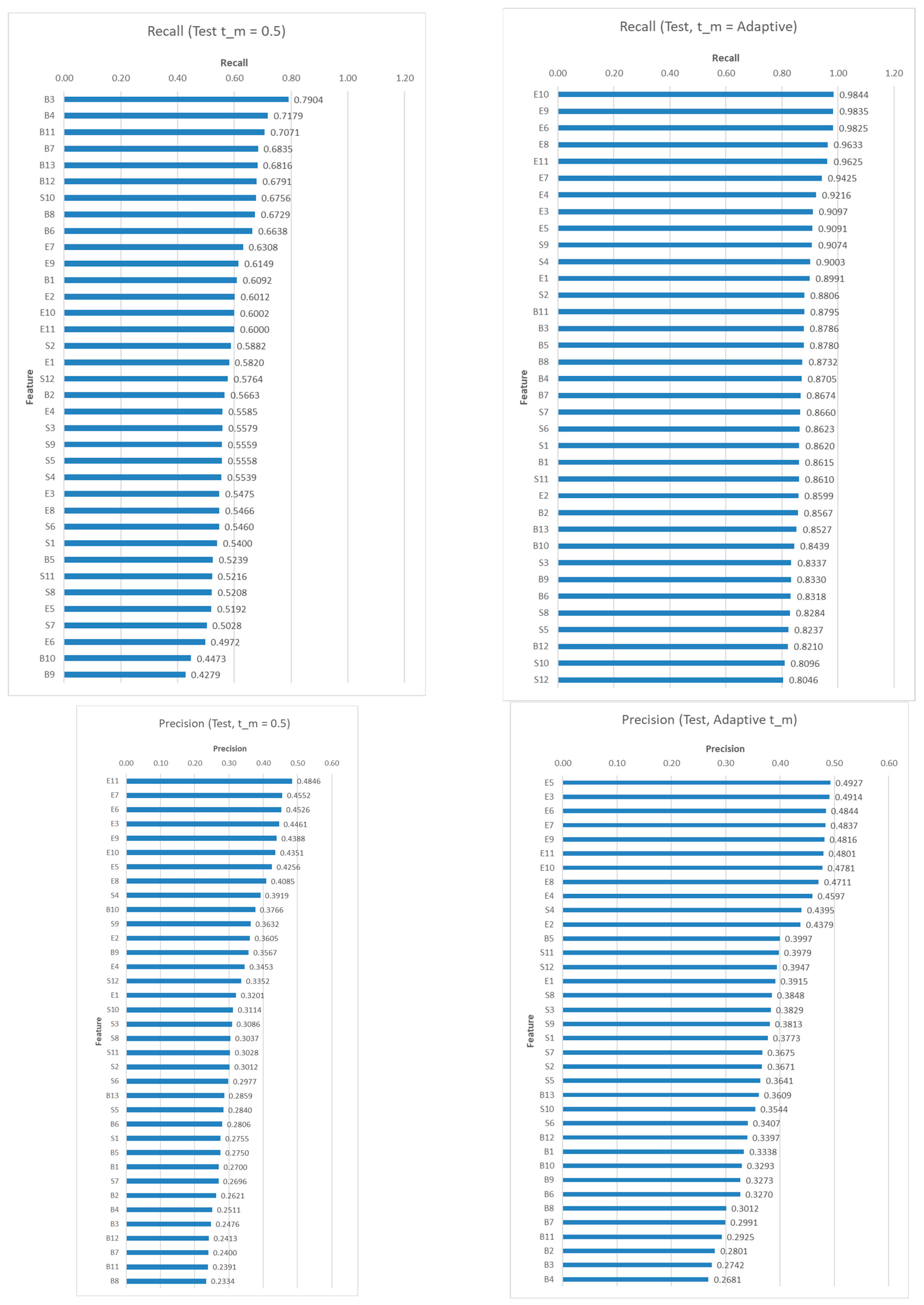
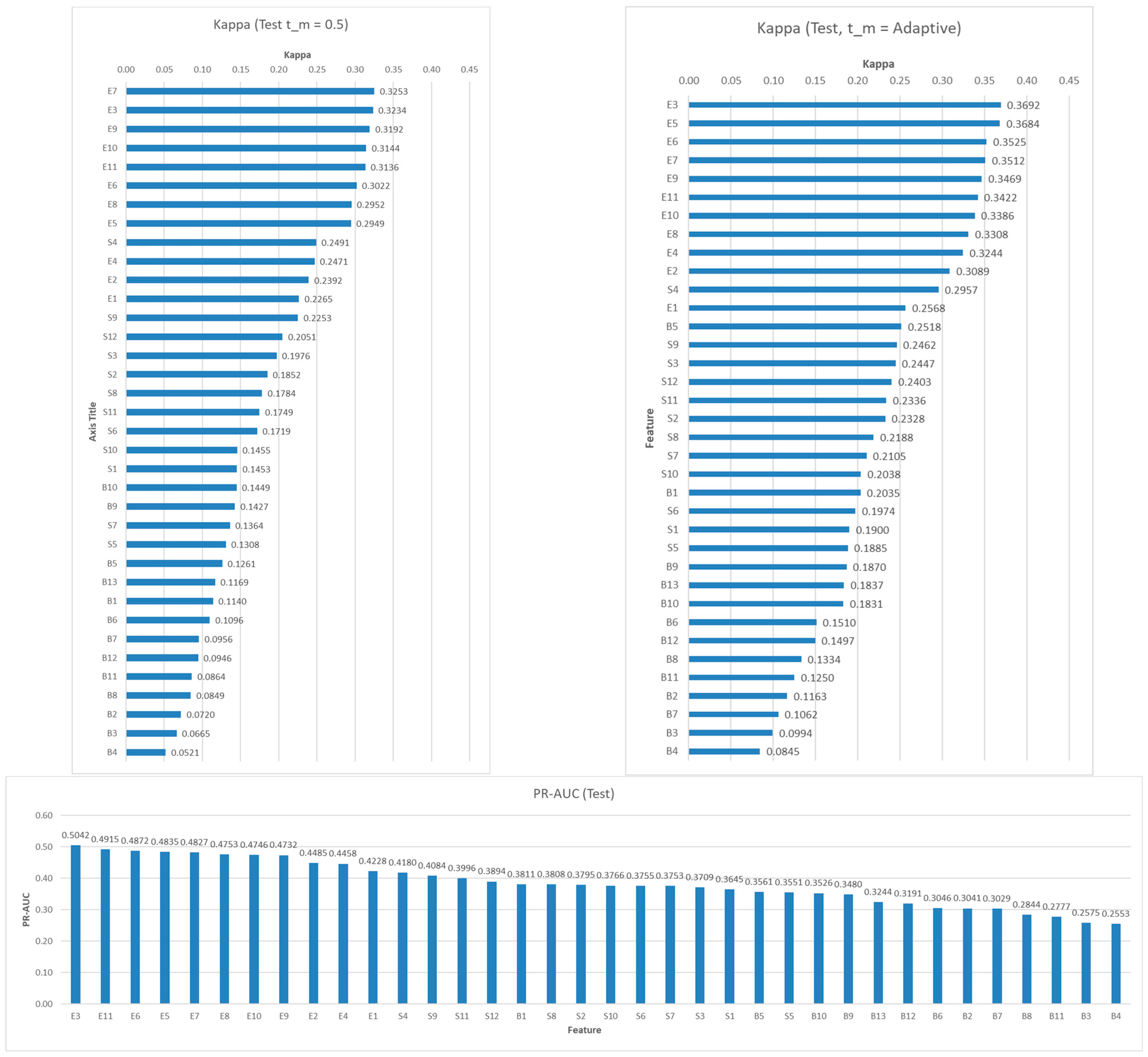
None of the plot features consistently outperformed the others across all evaluation metrics. In cross-validation, S9 (Hue + Hyper-hue-3D) achieved the top F1-scores, Kappa values, and PR-AUC (Figure A4). Hue effectively captured human-perceivable yellowing and browning caused by disease, and it was relatively robust to shadows and variable solar illumination. Hyper-hue extended this concept into the multispectral domain, enabling detection of subtle spectral shifts invisible to the human eye while remaining less sensitive to illumination changes [5,7]. In contrast, during cross-domain testing, feature E3 (Hue + NDVI + GNDVI + NDRE + TVI) provided superior performance in most evaluation metrics (Figure A5). GNDVI enhances sensitivity to chlorophyll concentration by using green rather than red reflectance, making it suitable for detecting early stress. NDRE leverages the red-edge region, which avoids saturation effects common in the red band and improves monitoring of chlorophyll content and canopy structure, particularly in dense vegetation. TVI reduces the influence of soil background and illumination variability, offering a more stable indicator of canopy greenness. Together, these vegetation indices support a more robust evaluation of plant vigour and stress responses under diverse environmental conditions. Ensemble learning, which integrates models trained on different plot-level features to further enhance predictive performance, represents a promising direction for future research.

4.4. Domain Shift

Domain shift (also known as distributional or dataset shift) occurs when the target domain distribution differs significantly from the source domain used during training [8]. In this study, skewed disease score distributions caused by different weather patterns during the growing season and locations of the field trials and disparate scoring methodologies were the primary drivers of domain shift.

In this study, by applying the adaptive classification thresholding strategy together with the most informative plot features, the decline in F1-score was reduced to only 8%, compared with an 18% drop under the fixed default classification threshold. This demonstrates a substantial improvement in model robustness and generalisation. Nevertheless, domain shift remains an open research problem that requires further in-depth investigation.

5. Conclusions

This study demonstrates that UAV-based RGB and multispectral imagery provides a high-throughput, cost-effective framework for estimating net blotch severity at the plot scale. Our findings indicate that the efficacy of these remote sensing models is heavily contingent upon the quality and distributional characteristics of the ground-truth data. We identified that adverse growing seasons with severe droughts and thus low infection levels at the Turretfield site significantly impact model performance. Furthermore, inconsistencies in human scoring protocols introduce label noise that complicates model convergence. A key technical insight from this research is that regression models for continuous disease severity score estimation remain highly challenging at the plot scale due to the skewed data distributions and biassed ground-truth scores. In contrast, the application of carefully selected thresholds yielded more robust and practical classification results for rapid screening. Cross-validation showed that, with properly engineered plot features, the models performed reasonably well within the same dataset. The cross-domain testing highlights the persistent challenge of domain shift in plant phenotyping. In this study, several factors contributed to the high false-negative rates observed under cross-domain evaluation, including the top-down perspective of UAV-based imaging, skewed data distributions, and potential biases in ground-truth disease scoring. Future work will focus on improving model generalisability by exploring advanced domain-adaptation techniques and leveraging synthetic training data to help bridge gaps in natural data distributions.

References

1. Rezaei, M.; Diepeveen, D.; Laga, H.; Jones, M.; Sohel, F. Plant disease recognition in a low data scenario using few-shot learning. Comput. Electron. Agric. 2024, 219, 108812. [Google Scholar] [CrossRef]
2. Alhashel, A.; Fiedler, J.; Nandety, R.; Skiba, R.; Bruggeman, R.; Baldwin, T.; Friesen, T.; Yang, S. Genetic and physical localization of a major susceptibility gene to Pyrenophora teres f. maculata in barley. Theor. Appl. Genet. 2023, 136, 118. [Google Scholar] [CrossRef] [PubMed]
3. Saraswathi, E.; Banu, J.; Hanne, T.; Bajaj, A.; Abraham, A.; Hong, T. Deep Learning Approaches for Disease Detection Based on Plant Leaf Image: A Review; Springer: Cham, Switzerland, 2024; Volume 1047, pp. 323–338. [Google Scholar] [CrossRef]
4. Sathya, K.; Balakrishnan, A.; Baskaran, P.; Kumar, R. Enhancing plant disease detection using attention-augmented residual networks and faster region-convolutional networks. IEEE Access 2025, 13, 48625–48642. [Google Scholar] [CrossRef]
5. Liu, H.; Lee, S.H.; Chahl, J.S. Transformation of a high-dimensional color space for material classification. J. Opt. Soc. Am. A 2017, 34, 523–532. [Google Scholar] [CrossRef] [PubMed]
6. Horsfall, G.; Barratt, R. An improved grading system for measuring plant diseases. Phytopathology 1945, 115, 655. [Google Scholar] [CrossRef] [PubMed]
7. Liu, H.; Lee, S.H.; Chahl, J.S. A multispectral 3D vision system for invertebrate detection on crops. IEEE Sens. J. 2017, 17, 7502–7515. [Google Scholar] [CrossRef]
8. Tunio, M.; Li, J.; Zeng, X.; Ahmed, A.; Shah, S.; Shaikh, H.; Mallah, G.; Yahya, I. Advancing plant disease classification: A robust and generalized approach with transformer-fused convolution and Wasserstein domain adaptation. Comput. Electron. Agric. 2024, 227, 109574. [Google Scholar] [CrossRef]
Figure 1. Plot feature extraction methods. Top row: The RGB orthomosaics are first converted from RGB colour space to HSV colour space, and then the histograms of hue are extracted as the plot feature. Bottom row: The multispectral orthomosaics are converted to VI images or HHSI colour space, and then the histograms of VI images and hyper-hue images are extracted to describe the plot features.
Blsf 57 00007 g001
Figure 2. The distributions of disease scores of the field trials. (a) Horsham 2023. (b) Horsham 2024. (c) Turretfield 2023. (d) Turretfield 2024.
Blsf 57 00007 g002
Figure 3. Cross-validation and cross-domain test results. (a) Cross-validation performance, where metric values were averaged across all plot features, domains, and disease-score thresholds. (b) Cross-validation performance based on the best-performing plot features in each evaluation metrics, after averaging across domains and disease-score thresholds. Results obtained using the default classification decision threshold tm = 0.5 are compared with those obtained using the adaptive thresholding strategy. (c,d) present the corresponding results for cross-domain testing.
Blsf 57 00007 g003
Disclaimer/Publisher’s Note: The statements, opinions and data contained in all publications are solely those of the individual author(s) and contributor(s) and not of MDPI and/or the editor(s). MDPI and/or the editor(s) disclaim responsibility for any injury to people or property resulting from any ideas, methods, instructions or products referred to in the content.