A Diseased Three-Species Harvesting Food Web Model with Various Response Functions ^†

Abstract

The purpose of this work is to present a three-species harvesting food web model that takes into account the interactions of susceptible prey, infected prey, and predator species. Prey species are assumed to expand logistically in the absence of predator species. The Crowley–Martin and Beddington–DeAngelis functional responses are used by predators to consume both susceptible and infected prey. Additionally, susceptible prey is consumed by infected prey in the formation of a Holling type II response. Both prey species are considered when prey harvesting is taken into account. Boundedness, positivity, and positive invariance are considered in this study. The investigation covers all the equilibrium points that are biologically feasible. Local stability is evaluated by analyzing the distribution of eigen values, while global stability is evaluated using suitable Lyapunov functions. Also, Hopf bifurcation is analyzed at the harvesting rate ${\mathcal{H}}_1$. At the end, we evaluate the numerical solutions based on our findings.

1. Introduction

In the natural environment, a variety of diseases may arise and spread among species when they interact with other organisms. Mathematical models have evolved into important tools for evaluating disease propagation and control. An eco-epidemiological model of diseased three-species food webs includes infectious prey, susceptible prey, and predators. At the beginning of the 20th century, several strategies were established in mathematical ecology to predict the presence of organisms and species of growth. The first significant attempt in this field was the well-known traditional Lotka–Volterra model [1] in 1927.

The investigation of predator–prey relationships is a crucial field of ecological research. The mathematical modeling of epidemics has become a prominent field of research. In this field, a substantial quantity of research has been performed [2,3,4]. Furthermore, mining and harvesting are practiced on a large number of the species found in the natural environment. Harvesting of the species is required for coexistence, and hence, the researchers were quite interested in the proposed ecological models. Different methods of harvesting have been proposed and explored, including constant harvesting, density-dependent proportional harvesting, and nonlinear harvesting [5,6]. By considering the above, in this work, we propose and study an eco-epidemiological prey–predator model involving different functional responses of harvesting. The majority of functional responses, like Holling types, are classified as “prey-dependent” because they depend on either the predator or the prey [7]. Both the prey and the predator are taken into account in Crowley–Martin reactions. In the Beddington–DeAngelis form, handling prey and hunting prey are viewed as two separate and independent actions. The response function of Beddington–DeAngelis, Holling type II, and Crowley–Martin forms are considered in this work. The main goal of this study is to analyze how disease and prey harvesting affect the predator–prey relationship. To the best of our knowledge, no studies have looked at an eco-epidemiological model of the three-species food web of harvesting with varying functional responses.

Section 2 addresses the mathematical expression. Some preliminary observations are presented in Section 3. The boundary equilibrium points and stability are shown in Section 4. In Section 5.1, the coexistence condition of the interior equilibrium point ${\mathcal{E}}^{*}(a^{*},i^{*},r^{*})$ is determined by examining its local stability. The global stability analysis for ${\mathcal{E}}^{*}$ is verified in Section 5.2. Furthermore, Section 6, investigates the Hopf bifurcation based on the harvesting rate ${\mathcal{H}}_1$. The MATLAB software tool (https://www.mathworks.com/products/matlab.html accessed on 1 March 2024) is used quantitatively to validate all the key results in Section 7. The conclusion of this research, as well as the environmental impacts of our results, are shown in Section 8, which ends our research.

2. Formation and Flowchart of the Equation

Prey harvesting is incorporated into the models for a predator–prey system.

$$\begin{array}{c}\hfill \left.\begin{array}{ccc}\frac{d\mathcal{A}}{d\mathcal{T}}& =& x_1\mathcal{A}(1-\frac{\mathcal{A}+\mathcal{I}}{K})-\frac{\pi \mathcal{A}\mathcal{I}}{s_1+\mathcal{A}}-\frac{{\alpha }_1\mathcal{A}\mathcal{R}}{(1+\eta \mathcal{A})(1+\mu \mathcal{R})}-{\mathcal{H}}_1{\mathcal{E}}_1\mathcal{A},\\ \frac{d\mathcal{I}}{d\mathcal{T}}& =& \frac{\pi \mathcal{A}\mathcal{I}}{s_1+\mathcal{A}}-d_1\mathcal{I}-\frac{g_1\mathcal{I}\mathcal{R}}{(1+\beta \mathcal{I}+\gamma \mathcal{R})}-{\mathcal{H}}_2{\mathcal{E}}_2\mathcal{I},\\ \frac{d\mathcal{R}}{d\mathcal{T}}& =& -d_2\mathcal{R}+\frac{m{\alpha }_1\mathcal{A}\mathcal{R}}{(1+\eta \mathcal{A})(1+\mu \mathcal{R})}+\frac{m{g}_1\mathcal{I}\mathcal{R}}{(1+\beta \mathcal{I}+\gamma \mathcal{R})},\end{array}\right\}\end{array}$$

(1)

by the positive conditions $\mathcal{A}\left(0\right)={\mathcal{A}}_0\ge 0,\mathcal{I}\left(0\right)={\mathcal{I}}_0\ge 0$, and $\mathcal{R}\left(0\right)={\mathcal{R}}_0\ge 0$. The detailed environmental illustrations of the parameters are given in Table 1.

Table 1. Ecological description of the model.

Parameters	Ecological Description
$\mathcal{R},\mathcal{A},\mathcal{I}$	predator species, susceptible prey, infected prey
$\pi$, x	infectious and growth rate of prey
K, $\eta$, $\mathcal{E}$	carrying capacity, handling time of predators, harvesting effort
$s_1$ and $\beta$	infected prey and predators half-saturation constant
$m,{\alpha }_1$	conversion of prey to predators, of susceptible prey’s predation rate
$\gamma ,\mu$	magnitude of interference by predators of Beddington and Crowley
$g_1$	consuming rate of susceptible prey by predator
$d_1$ and $d_2$	mortality rate infectious prey and predators
${\mathcal{H}}_1$, ${\mathcal{H}}_2$	susceptible and infected prey’s catchability coefficient

To minimize the parameters in model (1), we modify the variables as follows: $a=\frac{\mathcal{A}}{K},i=\frac{\mathcal{I}}{K},r=\frac{\mathcal{R}}{K}$ The transformations can be utilized to formulate the Equation (1) in a dimensionless form ($t=\pi \mathcal{T}\mathcal{K}$). Figure 1 displays the the model’s flowchart with the harvesting of various functional responses.

$$\begin{array}{c}\hfill \left.\begin{array}{ccc}\frac{da}{dt}& =& xa(1-a-i)-\frac{\pi ai}{s+a}-\frac{\alpha ar}{(1+\eta a)(1+\mu r)}-h_{1}a,\\ \frac{di}{dt}& =& \frac{\pi ai}{s+a}-di-\frac{\theta ir}{(1+\beta i+\gamma r)}-h_{2}i,\\ \frac{dr}{dt}& =& -\delta r+\frac{m\alpha ar}{(1+\eta a)(1+\mu r)}+\frac{m\theta ir}{(1+\beta i+\gamma r)}\end{array}\right\}\end{array}$$

(2)

where $x=\frac{x_1}{\pi K},\alpha =\frac{{\alpha }_1}{\pi K},s=\frac{s_1}{K},\theta =\frac{g_1}{\rho K},d=\frac{d_1}{\pi K},\delta =\frac{d_2}{\pi K}$. Now, the model’s conditions are $a\left(0\right)=a_0\ge 0,i\left(0\right)=i_0\ge 0$, and $r\left(0\right)=r_0\ge 0$.

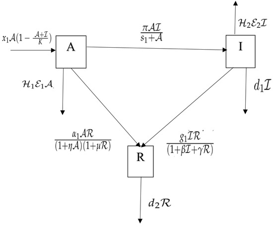
Figure 1. Flowchart of the model with different functional responses.

3. Positivity and Boundedness

Let $F\equiv {(a\left(t\right),i\left(t\right),r\left(t\right))}^T$ and $\mathcal{V}\left(F\right)={({\mathcal{V}}_1\left(F\right),{\mathcal{V}}_2\left(F\right),{\mathcal{V}}_3\left(F\right))}^T$, where

$$\begin{array}{cc}\hfill {\mathcal{V}}_1\left(F\right)& =xa(1-a-i)-\frac{\pi ai}{s+a}-\frac{\alpha ar}{(1+\eta a)(1+\mu r)}-h_{1}a,\hfill \\ \hfill {\mathcal{V}}_2\left(F\right)& =\frac{\pi ai}{s+a}-di-\frac{\theta ai}{(1+\beta i+\gamma a)}-h_{2}i,\hfill \\ \hfill {\mathcal{V}}_3\left(F\right)& =-\delta r+\frac{m\alpha ar}{(1+\eta a)(1+\mu r)}+\frac{m\theta ir}{(1+\beta i+\gamma r)}.\hfill \end{array}$$

The Equation can be denoted as $\frac{dF}{dt}=\mathcal{V}\left(F\right)$ where $\mathcal{V}:$$C_{+}\to {\mathcal{R}}_{+}^3$ with $F\left(0\right)=F_0\in {\mathcal{R}}_{+}^3.$ Thus, ${\mathcal{V}}_m\in {\mathcal{C}}^{\infty }\left(\mathcal{R}\right)$ for $m=1,2,3$. $\mathcal{V}$ is continuous and a Lipschitzian function on ${\mathcal{R}}_{+}^3$. It contains non-negative conditions. So, the region ${\mathcal{R}}_{+}^3$ is under an invariant condition.

Theorem 1.

The model’s (2) potential responses are bounded, and it is in ${\mathcal{R}}_{+}^3$.

Proof. 

Let $\left(a\right(t),i(t),r(t\left)\right)$ be the prescribed response for model (2).

Let $\frac{da}{dt}\le a(1-a).$

${lim\; sup}_{t\to \infty }$$a\left(t\right)\le 1.$ Let $\psi =a+i+r$.

$$\begin{array}{cc}\hfill \frac{d\psi }{dt}=& xa(1-a)-ai(x+\frac{\pi }{s+a})-\frac{\alpha ar(1-m)}{(1+\eta a)(1+\mu r)}-h_{1}a+\frac{ai}{s+a}-di\hfill \\ \hfill & -\frac{\theta ir}{(1+\beta i+\gamma r)}(1-m)-h_{2}i-\delta r,\hfill \\ \hfill \le & xa(1-a)-h_{1}a-air-i(d+h_2)-\delta r,(sincem<1)),\hfill \\ \hfill \le & \frac{x}{4}-h_{1}a-i(d+h_2)-\delta r(sinceMax\left\{xa(1-a)\right\}=\frac{x}{4}),\hfill \\ \hfill \le & \frac{x}{4}-\beta \psi .where,\beta =min\{h_1,d+h_2,\delta \}.\hfill \end{array}$$

Thus, $\frac{d\psi }{dt}+\beta \psi \le \frac{x}{4}.$ We have $0<\psi \le \frac{x}{4\beta }(1-{exp}^{-\beta t})+\psi (a_0,i_0,r_0){exp}^{-\beta t}.$ If $t\to \infty$, because 0 <$\psi$≤$\frac{x}{4\beta }$. Hence, the solutions of model (2) are confined to a positive around $\mathsf{\Omega }$,

where $\mathsf{\Omega }$ = $\{(a,i,r)\in {\mathcal{R}}_{+}^3:a+i+r\le \frac{x}{4\beta }+\in \}.$ □

4. Presence of Boundary Equilibrium Points

• ${\mathcal{E}}_0$ is the equilibria of a trivial point. Here, ${\mathcal{E}}_0$ (0, 0, 0) exists.
• ${\mathcal{E}}_1$ is no infection and predator-free equilibria; ${\mathcal{E}}_1$ $(\frac{x-h_1}{x},0,0)$ exists for $h_1$ < $x.$
• ${\mathcal{E}}_2$ is the equilibria of without a predator; ${\mathcal{E}}_2$$(\overline{a},\overline{i},0)$ where $\overline{a}$ = $\frac{s(d+h_2)}{(1-d-h_2)}$ and
  $\overline{i}$ = $\frac{(x(1-a)-h_1)(s+a)}{x}$. ${\mathcal{E}}_2$ exists for $s(d+h_2)<(1-d-h_2)$ and $h_1<x(1-a)$.
• ${\mathcal{E}}_3$ is the no diseases of the equilibria; ${\mathcal{E}}_3$ $(\overline{a},0,\overline{r})$ where $\overline{a}$ = $\frac{\delta (1+\mu r)}{m\alpha -\eta \delta (1+\mu r)}$ and
  $\overline{r}$ = $\frac{(x(1-a)-h_1)(1+\eta a)(1+\mu )}{\alpha }$. ${\mathcal{E}}_3$ exists for $\eta \delta (1+\mu r)<m\alpha$ and $h_1<x(1-a)$.
• ${\mathcal{E}}^{*}$ is the equilibria of the coexistent state; ${\mathcal{E}}^{*}$$(a^{*},i^{*},r^{*})$. It exists for $\delta >m\alpha$, $(1+\beta i^{*}+\gamma r^{*})>0$, $x(1-a^{*}-i^{*})>h_1-i^{*}$, $\alpha s>0$, where
  $a^{*}$ =$\frac{s+((d+h_2)+(1+\beta i^{*}+\gamma r^{*})+\theta r^{*})}{(1+\beta i^{*}+\gamma r^{*})}$, $i^{*}$ =$\frac{(1+\beta +\gamma r^{*})(\delta (1+\eta a^{*})(1+\mu r^{*})-m\alpha a^{*})}{(1+\eta a^{*})(1+\mu r^{*})m\theta }$, and
  $r^{*}$ =$\frac{\left((1+\eta a^{*})(1+\mu )\right)(s+a^{*}(x(1-a^{*}-i^{*})-h_1)-i^{*})}{\alpha (s+a^{*})}$.

5. Stability Analysis

5.1. Local Analysis

The matrix of Jacobian equations is used to investigate the local stability at a point in $(a,i,r)$, which is

$$\begin{array}{cc}\hfill n_{11}=& x(1-2a-i)-\frac{si}{{(s+a)}^2}-\frac{\alpha r}{{(1+\eta a)}^2(1+\mu r)}-h_1,n_{12}=-ax-\frac{a}{a+s},\hfill \\ \hfill n_{13}=& -\frac{\alpha a}{{(1+\mu r)}^2{(1+\eta a)}^2},n_{21}=\frac{si}{{(s+a)}^2},n_{31}=\frac{\alpha xm}{{(1+\eta a)}^2(1+\mu r)},\hfill \\ \hfill n_{22}=& \frac{a}{a+s}-d-\frac{x\theta (1+\gamma r)}{{(1+\beta i+\gamma r)}^2}-h_2,n_{23}=-\frac{i\theta (1+\beta i)}{{(1+\beta i+\gamma r)}^2},\hfill \\ \hfill n_{32}=& \frac{\theta xm(1+\gamma r)}{{(1+\beta i+\gamma r)}^2},n_{33}=-\delta +\frac{\alpha am}{{(1+\mu r)}^2(1+\eta a)}+\frac{\theta im(1+\beta i)}{{(1+\beta i+\gamma r)}^2}.\hfill \end{array}$$

Theorem 2.

The following are the points to verify the stability condition of model (2). They are as follows:

1. 

The trivial point of equilibria ${\mathcal{E}}_0(0,0,0)$ is LAS if $x<h_1$.

2. 

The infectious and predator-free points ${\mathcal{E}}_1(\frac{x-h_1}{x},0,0)$ are LAS if $x<h_1$, $-d-h_2>\frac{x-h_1}{x-h_1+s}$, and $\delta <\frac{(x-h_1)m\alpha }{1+\eta (x-h_1)}$.

3. 

The equilibria with no predator $(\overline{a},\overline{i},0)$ is LAS if ${\mathcal{Y}}_{11}>0$, ${\mathcal{Y}}_{12}>0$, and $\delta >\frac{m\alpha \overline{a}}{1+\eta \overline{a}}+\frac{\overline{i}m\theta (1+\beta \overline{i})}{{(\beta \overline{i}+1)}^2}$.

Proof. 

• The trivial point of equilibria ${\mathcal{E}}_0(0,0,0)$ of the eigen values are $x-h_1$, $-d-h_2$, and −δ. Hence, it is LAS when $x<h_1$; if not, it is unstable.
• The eigen values of ${\mathcal{E}}_1(\frac{x-h_1}{x},0,0)$ are $h_1-x$, $\frac{(x-h_1)}{(x-h_1)+s}-d-h_2$, and $\delta +\frac{(x-h_1)m\alpha }{1+\eta (x-h_1)}$. Hence, it is LAS if $x<h_1$, $-d-h_2>\frac{(x-h_1)}{(x-h_1)+s}$, and $\delta <\frac{(x-h_1)m\alpha }{1+\eta (x-h_1)}$; if not, it is unstable.
• The matrix in its Jacobian form is

  $$\begin{array}{cc}\hfill n_{11}=& x(1-2\overline{a}-\overline{i})-\frac{s\overline{i}}{{(s+\overline{a})}^2}-h_1,n_{12}=-\overline{a}x-\frac{\overline{a}}{\overline{a}+s},n_{13}=-\frac{\alpha \overline{a}}{1+\eta \overline{a}},\hfill \\ \hfill n_{21}=& \frac{s\overline{i}}{{(s+\overline{a})}^2},n_{22}=\frac{\overline{a}}{\overline{a}+s}-d-h_2,n_{23}=-\frac{\overline{i}\theta (1+\beta i)}{{(\beta \overline{i}+1)}^2},n_{31}=0,n_{32}=0,\hfill \\ \hfill n_{33}=& -\delta +\frac{\overline{a}m\alpha }{1+\eta \overline{a}}+\frac{im\theta (1+\beta i)}{{(\beta i+1)}^2}.\hfill \end{array}$$

The characteristic form of $J\left({\mathcal{E}}_2\right)$ is $(n_{33}-\lambda )({\lambda }^2+{\mathcal{S}}_{11}\lambda +{\mathcal{S}}_{12})=0$, where ${\mathcal{S}}_{11}=-(n_{11}+n_{22})$ and ${\mathcal{S}}_{12}=n_{11}{n}_{22}-n_{12}{n}_{21}$. As a result, one of the eigenvalues of the equation is $n_{33}$, i.e., negative. Hence, the other two must likewise be negative. So, ${\mathcal{E}}_2$ is LAS if ${\mathcal{S}}_{11}>0$, ${\mathcal{S}}_{12}>0$, and $\delta >\frac{\overline{a}m\alpha }{1+\eta \overline{a}}+\frac{im\theta (1+\beta i)}{{(\beta i+1)}^2}$. □

Theorem 3.

The infectious-free point of equilibrium $(\overline{a},0,\overline{r})$ is LAS if ${\mathcal{D}}_{11}>0$, ${\mathcal{D}}_{12}>0$, and $-(d+\frac{r\theta (1+\gamma r)}{{(\beta b+\gamma r+1)}^2}+h_2)>\frac{a}{a+s}$.

(This demonstration is equivalent to Theorem 2, condition (3).)

Theorem 4.

The equilibrium point ${\mathcal{E}}^{*}$ is LAS if ${\mathcal{G}}_1>0$, ${\mathcal{G}}_3>0$, and ${\mathcal{G}}_1{\mathcal{G}}_2-{\mathcal{G}}_3>0$.

Proof. 

As for model (2), its Jacobian matrix is at ${\mathcal{E}}^{*}(a^{*},i^{*},r^{*})$.

$$\begin{array}{cc}\hfill g_{11}=& x(1-2a^{*}-i^{*})-\frac{s{i}^{*}}{{(s+a^{*})}^2}-\frac{\alpha r^{*}}{{(1+\eta a^{*})}^2(1+\mu r^{*})}-h_1,\hfill \\ \hfill g_{12}=& -a^{*}x-\frac{a^{*}}{a^{*}+p},g_{13}=-\frac{\alpha a^{*}}{{(1+\mu r^{*})}^2{(1+\eta a^{*})}^2},g_{21}=\frac{s{i}^{*}}{{(s+a^{*})}^2},\hfill \\ \hfill g_{31}=& \frac{\alpha r^{*}m}{{(1+\eta a^{*})}^2(1+\mu r^{*})},g_{22}=\frac{a^{*}}{a^{*}+s}-d-\frac{r^{*}\theta (1+\gamma r^{*})}{{(1+\beta i^{*}+\gamma r^{*})}^2}-h_2,\hfill \\ \hfill g_{23}=& -\frac{i^{*}\theta (1+\beta i^{*})}{{(1+\beta i^{*}+\gamma r^{*})}^2},g_{32}=\frac{\theta r^{*}m(1+\gamma r^{*})}{{(1+\beta i^{*}+\gamma r^{*})}^2},g_{33}=0\hfill \end{array}$$

The cubic characteristic equation $J\left({\mathcal{E}}^{*}\right)$ is

$${\lambda }^3+{\mathcal{G}}_1{\lambda }^2+{\mathcal{G}}_2\lambda +{\mathcal{Y}}_3=0.$$

(3)

${\mathcal{G}}_1=-(g_{11}+g_{22})$, ${\mathcal{G}}_2=-(g_{12}{g}_{21}+g_{13}{g}_{31}+g_{23}{g}_{32}-g_{11}{g}_{22}-g_{11}{g}_{33});$

${\mathcal{G}}_3=-(g_{12}{g}_{23}{g}_{31}+g_{13}{g}_{21}{g}_{32}-g_{13}{g}_{31}{g}_{22}-g_{11}{g}_{23}{g}_{32}).$

${\mathcal{G}}_1>0$, ${\mathcal{G}}_3>0$, and ${\mathcal{G}}_1{\mathcal{G}}_2-{\mathcal{G}}_3>0$. The root of the characteristic equation is negative real parts if and only if ${\mathcal{G}}_1$, ${\mathcal{G}}_3$, and ${\mathcal{G}}_1{\mathcal{G}}_2-{\mathcal{G}}_3>0$. According to Routh–Hurwitz, ${\mathcal{E}}^{*}$ is LAS. □

5.2. Global Analysis

Theorem 5.

The point ${\mathcal{E}}^{*}$ is GAS in $W=\{(a,i,r):a>a^{*},i>i^{*}$ and $r>r^{*}$ or $a<a^{*},i<i^{*}$ and $r<r^{*}\}$.

Proof. 

A suitable Lyapunov function is expressed as

${\displaystyle {\mathcal{N}}_1(a,i,r)={\mathcal{N}}_2(a-a^{*}-a^{*}ln\frac{a}{a^{*}})+(i-i^{*}-i^{*}ln\frac{i}{i^{*}})+{\mathcal{N}}_3(r-r^{*}-r^{*}ln\frac{r}{r^{*}})}$,

where ${\mathcal{N}}_2,{\mathcal{N}}_3$ are positive constant.

Differentiating ${\mathcal{N}}_1$ with regard to t,

$\begin{array}{l}\frac{d{\mathcal{N}}_1}{dt}=\left(\frac{a-a^{*}}{a}\right)\frac{da}{dt}+{\mathcal{N}}_2\left(\frac{i-i^{*}}{i}\right)\frac{di}{dt}+{\mathcal{N}}_3\left(\frac{r-r^{*}}{r}\right)\frac{dr}{dt}\\ =[x(1-a-i)-\frac{\pi i}{s+a}-\frac{\alpha r}{(1+\eta a)(1+\mu r)}-h_1](a-a^{*})+{\mathcal{N}}_2[\frac{\pi a}{s+a}-d-\frac{\theta r}{(1+\beta i+\gamma r)}-h_2](i-i^{*})\\ +{\mathcal{N}}_3[-\delta +\frac{m\alpha a}{(1+\eta a)(1+\mu r)}+\frac{m\theta i}{(1+\beta i+\gamma r}](r-r^{*}).\end{array}$

$\begin{array}{l}\frac{d{\mathcal{N}}_1}{dt}=-(a-a^{*})[x(a+i)-(a^{*}+i^{*})]-\pi (\frac{i}{s+a}-\frac{i^{*}}{s+a^{*}})-\alpha (\frac{r}{(1+\eta a)(1+\mu r)}-\frac{r^{*}}{(1+\eta a^{*})(1+\mu r^{*})})]\\ -{\mathcal{N}}_2(i-i^{*})[(\frac{a}{(s+a)}-\frac{a^{*}}{(s+a^{*})})-\theta (\frac{r}{a+(1+\beta i+\gamma r)}-\frac{r^{*}}{1+\beta i^{*}+\gamma r^{*}}]\\ -{\mathcal{N}}_3(r-r^{*})m[\left(\frac{\alpha (a-a^{*})+r{\mu }^{*}(a-a^{*})}{(1+\eta a)(1+\mu r)(1+\eta a^{*})(1+\mu r^{*})}\right)-\theta \left(\frac{(i-i^{*})+\gamma (i{r}^{*}-i^{*}r)}{(1+\beta i+\gamma r)(1+\beta i^{*}+\gamma r^{*})}\right)].\end{array}$

The region area $\mathcal{N}$ and $\frac{d{\mathcal{N}}_1}{dt}$ is negative:

$W=\{(a,i,r):a>a^{*},i>i^{*}andr>r^{*})ora<a^{*},i<i^{*}andr<r^{*}\}$ and it shows that $\mathcal{N}$ is a suitable Lyapunov function for all the solutions in W. □

6. Analysis of the Hopf Bifurcation

Theorem 6.

If the bifurcating parameter ${\mathcal{H}}_1$ exceeds a substantial value, then Hopf bifurcation occurs in the system (2). The presence of the Hopf bifurcation requirements listed below is ${\mathcal{H}}_1$ = ${\mathcal{H}}_1^{*}$

1. 

$\mathcal{X}\left({\mathcal{H}}_1^{*}\right)\mathcal{R}\left({\mathcal{H}}_1^{*}\right)-\mathcal{D}\left({\mathcal{H}}_1^{*}\right)=0;$

2. 

$\frac{d}{d{\mathcal{H}}_1}\left(Re\left(\gamma \left({\mathcal{H}}_1\right)\right)\right){|}_{{\mathcal{H}}_1={\mathcal{H}}_1^{*}}\ne 0,$ where γ represents the positive value of the equilibrium point and is the zero of the characteristic equation.

Proof. 

For ${\mathcal{H}}_1={\mathcal{H}}_1^{*}$, let (3) denote

$({\gamma }^2\left({\mathcal{H}}_1^{*}\right)+\mathcal{R}\left({\mathcal{H}}_1^{*}\right))(\gamma \left({\mathcal{H}}_1^{*}\right)+\mathcal{X}\left({\mathcal{H}}_1^{*}\right))=0.$ (i.e) $\pm i\sqrt{\mathcal{R}\left({\mathcal{H}}_1^{*}\right)}$ and $-\mathcal{X}\left({\mathcal{H}}_1^{*}\right)$ are the roots of the Equation (6). To establish that the Hopf bifurcation exists at the point, we must fulfill the transversality requirement. ${\mathcal{H}}_1^{*}={\mathcal{H}}_1$. $\frac{d}{d{\mathcal{H}}_1}\left(Re\left(\gamma \left({\mathcal{H}}_1\right)\right)\right){|}_{{\mathcal{H}}_1={\mathcal{H}}_1^{*}}\ne 0.$ For all ${\mathcal{H}}_1$, the roots of the form ${\gamma }_1{,}_2\left({\mathcal{H}}_1\right)=r\left({\mathcal{H}}_1\right)\pm is\left({\mathcal{H}}_1\right),$ and ${\gamma }_3\left({\mathcal{H}}_1\right)=-\mathcal{X}\left({\mathcal{H}}_1\right).$ Now, we check the condition $\frac{d}{d{\mathcal{H}}_1}\left(Re\left({\gamma }_j\left({\mathcal{H}}_1\right)\right)\right){|}_{{\mathcal{H}}_1={\mathcal{H}}_1^{*}}\ne 0,j=1,2.$ Let ${\gamma }_1\left({\mathcal{H}}_1\right)$= $r\left({\mathcal{H}}_1\right)+is\left({\mathcal{H}}_1\right)$ in (6), and we obtain ${\gamma }_1\left({\mathcal{H}}_1\right)+i{\gamma }_2\left({\mathcal{H}}_1\right)=0,$ where

${\gamma }_1\left({\mathcal{H}}_1\right)=r^3\left({\mathcal{H}}_1\right)+r^2\left({\mathcal{H}}_1\right)\mathcal{X}\left({\mathcal{H}}_1\right)-3r\left({\mathcal{H}}_1\right)s^2\left({\mathcal{H}}_1\right)-s^2\left({\mathcal{H}}_1\right)\mathcal{X}\left({\mathcal{H}}_1\right)+r\left({\mathcal{H}}_1\right)\mathcal{R}\left({\mathcal{H}}_1\right)+\mathcal{X}\left({\mathcal{H}}_1\right)\mathcal{R}\left({\mathcal{H}}_1\right)$, and ${\gamma }_2\left({\mathcal{H}}_1\right)=3r^2\left({\mathcal{H}}_1\right)s\left({\mathcal{H}}_1\right)+2r\left({\mathcal{H}}_1\right)s\left({\mathcal{H}}_1\right)\mathcal{X}\left({\mathcal{H}}_1\right)-s^3\left({\mathcal{H}}_1\right)+s\left({\mathcal{H}}_1\right)\mathcal{R}\left({\mathcal{H}}_1\right)$. To complete the Equation (6), we need ${\gamma }_1\left({\mathcal{H}}_1\right)=0$ and ${\gamma }_2\left({\mathcal{H}}_1\right)=0,$ and then we differentiate ${\gamma }_1$ and ${\gamma }_2$ with respect to ${\mathcal{H}}_1$. Because

$$\frac{d{\gamma }_1}{d{\mathcal{H}}_1}={\mathcal{N}}_1\left({\mathcal{H}}_1\right)r^{\prime }\left({\mathcal{H}}_1\right)-{\mathcal{N}}_2\left({\mathcal{H}}_1\right)s^{\prime }\left({\mathcal{H}}_1\right)+{\mathcal{N}}_3\left({\mathcal{H}}_1\right)=0,$$

(4)

$$\frac{d{\gamma }_2}{d{\mathcal{H}}_1}={\mathcal{N}}_2\left({\mathcal{H}}_1\right)r^{\prime }\left({\mathcal{H}}_1\right)+{\mathcal{N}}_1\left({\mathcal{H}}_1\right)s^{\prime }\left({\mathcal{H}}_1\right)+{\mathcal{N}}_4\left({\mathcal{H}}_1\right)=0,$$

(5)

$$\begin{array}{c}{\mathcal{N}}_1\left({\mathcal{H}}_1\right)=3r^2\left({\mathcal{H}}_1\right)+2r\left({\mathcal{H}}_1\right)\mathcal{X}\left({\mathcal{H}}_1\right)-3s^2\left({\mathcal{H}}_1\right)+\mathcal{R}\left({\mathcal{H}}_1\right),\hfill \\ {\mathcal{N}}_2\left({\mathcal{H}}_1\right)=6r\left({\mathcal{H}}_1\right)s\left({\mathcal{H}}_1\right)+2s\left({\mathcal{H}}_1\right)\mathcal{X}\left({\mathcal{H}}_1\right),\hfill \\ {\mathcal{N}}_3\left({\mathcal{H}}_1\right)=r^2\left({\mathcal{H}}_1\right){\mathcal{X}}^{\prime }\left({\mathcal{H}}_1\right)-s^2\left({\mathcal{H}}_1\right){\mathcal{X}}^{\prime }\left({\mathcal{H}}_1\right)+{\mathcal{D}}^{\prime }\left({\mathcal{H}}_1\right)+{\mathcal{R}}^{\prime }\left({\mathcal{H}}_1\right)r\left({\mathcal{H}}_1\right),\hfill \\ {\mathcal{N}}_4\left({\mathcal{H}}_1\right)=2r\left({\mathcal{H}}_1\right)s\left({\mathcal{H}}_1\right){\mathcal{X}}^{\prime }\left({\mathcal{H}}_1\right)+s\left({\mathcal{H}}_1\right){\mathcal{R}}^{\prime }\left({\mathcal{H}}_1\right).\hfill \end{array}$$

$$r^{\prime }\left({\mathcal{H}}_1\right)=-\frac{{\mathcal{N}}_1\left({\mathcal{H}}_1\right){\mathcal{N}}_3\left({\mathcal{H}}_1\right)+{\mathcal{N}}_2\left({\mathcal{H}}_1\right){\mathcal{N}}_4\left({\mathcal{H}}_1\right)}{{\mathcal{N}}_1^2\left({\mathcal{H}}_1\right)+{\mathcal{N}}_2^2\left({\mathcal{H}}_1\right)}.$$

(6)

$r\left({\mathcal{H}}_1\right)=0$ and $s\left({\mathcal{H}}_1\right)=\sqrt{\mathcal{R}\left({\mathcal{H}}_1\right)}$ at ${\mathcal{H}}_1={\mathcal{H}}_1^{*}$ on ${\mathcal{N}}_1\left({\mathcal{H}}_1\right),{\mathcal{N}}_2\left({\mathcal{H}}_1\right),{\mathcal{N}}_3\left({\mathcal{H}}_1\right)$ and ${\mathcal{N}}_4\left({\mathcal{H}}_1\right)$. So, ${\mathcal{N}}_1\left({\mathcal{H}}_1^{*}\right)=-2\mathcal{R}\left({\mathcal{H}}_1^{*}\right),{\mathcal{N}}_2\left({\mathcal{H}}_1^{*}\right)=2\sqrt{\mathcal{R}\left({\mathcal{H}}_1^{*}\right)}\mathcal{X}\left({\mathcal{H}}_1^{*}\right),{\mathcal{N}}_3\left({\mathcal{H}}_1^{*}\right)=-\mathcal{R}\left({\mathcal{H}}_1^{*}\right){\mathcal{X}}^{\prime }\left({\mathcal{H}}_1^{*}\right)+{\mathcal{D}}^{\prime }\left({\mathcal{H}}_1^{*}\right)$, ${\mathcal{N}}_4\left({\mathcal{H}}_1^{*}\right)=\sqrt{\mathcal{R}\left({\mathcal{H}}_1^{*}\right)}{\mathcal{R}}^{\prime }\left({\mathcal{H}}_1^{*}\right).$

$$r^{\prime }\left({\mathcal{H}}_1^{*}\right)=\frac{{\mathcal{D}}^{\prime }\left({\mathcal{H}}_1^{*}\right)-(\mathcal{X}\left({\mathcal{H}}_1^{*}\right){\mathcal{R}}^{\prime }\left({\mathcal{H}}_1^{*}\right)+\mathcal{R}\left({\mathcal{H}}_1^{*}\right){\mathcal{X}}^{\prime }\left({\mathcal{H}}_1^{*}\right))}{2({\mathcal{R}}^2\left({\mathcal{H}}_1^{*}\right)+{\mathcal{X}}^2\left(v^{*}\right))},$$

(7)

${\mathcal{D}}^{\prime }\left({\mathcal{H}}_1^{*}\right)-(\mathcal{X}\left({\mathcal{H}}_1^{*}\right){\mathcal{R}}^{\prime }\left({\mathcal{H}}_1^{*}\right)+\mathcal{R}\left({\mathcal{H}}_1^{*}\right){\mathcal{X}}^{\prime }{\mathcal{H}}_1^{*}))\ne 0,$

(i.e) $\frac{d}{d{\mathcal{H}}_1}\left(Re\left({\gamma }_j\left({\mathcal{H}}_1\right)\right)\right){|}_{{\mathcal{H}}_1={\mathcal{H}}_1^{*}}=r^{\prime }\left({\mathcal{H}}_1^{*}\right)\ne 0.j=1,2,$ and ${\gamma }_3\left({\mathcal{H}}_1^{*}\right)=-\mathcal{X}\left({\mathcal{H}}_1^{*}\right)\ne 0$.

Thus, the condition ${\mathcal{J}}^{\prime }\left({\mathcal{H}}_1^{*}\right)-(\mathcal{X}\left({\mathcal{H}}_1^{*}\right){\mathcal{R}}^{\prime }\left({\mathcal{H}}_1^{*}\right)+\mathcal{R}\left({\mathcal{H}}_1^{*}\right){\mathcal{X}}^{\prime }\left({\mathcal{H}}_1^{*}\right))\ne 0$. It has been confirmed that the transversality criteria apply to system (2), and the Hopf bifurcation occurs at ${\mathcal{H}}_1={\mathcal{H}}_1^{*}.$ □

7. Numerical Calculations of the Model

To verify the theoretical conclusions, this part performs a calculation on system (2). Here, the harvesting rate ${\mathcal{H}}_1$ is employed as an adjustable element. The simulation is accomplished by utilizing MATLAB software tools for the fixed parameter. Here, x = 0.2, $\delta$ = 0.1, d = 0.2, $\theta$ = 0.21, $\pi$ = (variable), $\eta$ = 0.13, $\alpha$ = 0.3, and $\mu$ = 0.11. If ${\mathcal{H}}_1$ is 0.21, when bifurcation occurs, the model (2) for the non-negative equilibrium is LAS ${\mathcal{E}}^{*}$(0.52764, 0.0916818, and 0.203662) and the rest of the adjustable elements have identical values. The model’s (2) stability is lost by increasing the bifurcation adjustable element to ${\mathcal{H}}_1$ = 0.47, leading to being LAU at ${\mathcal{E}}^{*}$(0.53824, 0.0917748, and 0.320178). Model (2) is able to pass the transversality conditions for $\left(Re\left(\gamma \left({\mathcal{H}}_1\right)\right)\right){|}_{{\mathcal{H}}_1={\mathcal{H}}_1^{*}}=0.002195\ne 0$. Hence, Figure 2 displays how the model’s behavior changes at a harvesting rate of ${\mathcal{H}}_1$ = 0.47.

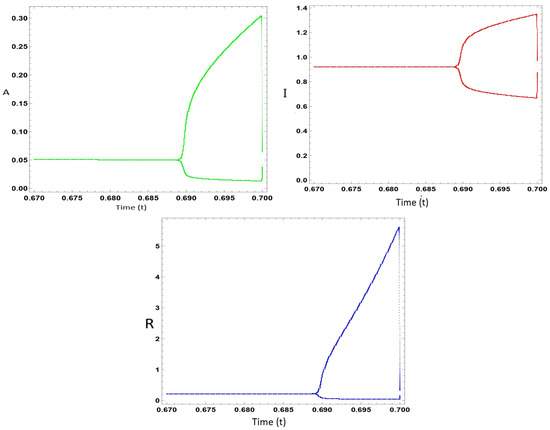
Figure 2. Dynamical changes in Model (2) at harvesting rate ${\mathcal{H}}_1$ = 0.47.

8. Conclusions and Discussion

Our investigation involved examining an eco-epidemiological model where sick prey are harvested from the prey species, and the predator eats both sick and healthy prey. The developed system (2) has been shown to be biologically well behaved by the boundedness and positivity results. In the event that if the growing rate of uninfected prey is lower than the harvest rate, then the population tends to be extinct. It has been demonstrated that both the local stability at every ecologically possible point and the coexistence (2) are stable. The analytical and numerical outcomes of the Hopf bifurcation for the harvesting rate ${\mathcal{H}}_1$ have been analyzed and evaluated in the above. The dynamic of prey harvesting is powerful due to the complex behavior demonstrated in this study. Thus, we believe that ordinary differential equations will be utilized to solve many future technological equations.

References

- May, R.M. Stability and Complexity in Model Ecosystems; Princeton University Press: Princeton, NJ, USA, 2019; Volume 1. [Google Scholar]
- Kant, S.; Kumar, V. Dynamics of a Prey-Predator System with Infection in Prey; Department of Mathematics, Texas State University: San Marcos, TX, USA, 2017. [Google Scholar]
- Pradeep, M.S.; Gopal, T.N.; Magudeeswaran, S.; Deepak, N.; Muthukumar, S. Stability analysis of diseased preadator–prey model with holling type II functional response. AIP Conf. Proc. 2023, 2901, 030017. [Google Scholar]
- Thangavel, M.; Thangaraj, N.G.; Manickasundaram, S.P.; Arunachalam, Y. An Eco–Epidemiological Model Involving Prey Refuge and Prey Harvesting with Beddington–DeAngelis, Crowley–Martin and Holling Type II Functional Responses. Eng. Proc. 2023, 56, 325. [Google Scholar] [CrossRef]
- Abdulghafour, A.S.; Naji, R.K. The impact of refuge and harvesting on the dynamics of prey-predator system. Sci. Int. 2018, 30, 315–323. [Google Scholar]
- Agnihotri, K.B.; Gakkhar, S. The dynamics of disease transmission in a prey predator system with harvesting of prey. Int. J. Adv. Res. Comput. Eng. Technol. 2012, 1, 1–17. [Google Scholar]
- Magudeeswaran, S.; Vinoth, S.; Sathiyanathan, K.; Sivabalan, M. Impact of fear on delayed three species food-web model with Holling type-II functional response. Int. J. Biomath. 2022, 15, 2250014. [Google Scholar] [CrossRef]
Disclaimer/Publisher’s Note: The statements, opinions and data contained in all publications are solely those of the individual author(s) and contributor(s) and not of MDPI and/or the editor(s). MDPI and/or the editor(s) disclaim responsibility for any injury to people or property resulting from any ideas, methods, instructions or products referred to in the content. |
© 2024 by the authors. Licensee MDPI, Basel, Switzerland. This article is an open access article distributed under the terms and conditions of the Creative Commons Attribution (CC BY) license (https://creativecommons.org/licenses/by/4.0/).