Author Contributions
Conceptualization, J.E., M.P. and S.G.; methodology, J.E., M.P. and S.G.; software, O.L.; validation, O.L.; formal analysis, J.E., M.P. and S.G.; investigation, J.E., M.P. and S.G.; resources, S.G.; data curation, O.L.; writing—original draft preparation, O.L.; writing—review and editing, S.G.; visualization, S.G.; supervision, J.E., M.P. and S.G.; project administration, S.G.; funding acquisition, S.G. All authors have read and agreed to the published version of the manuscript.
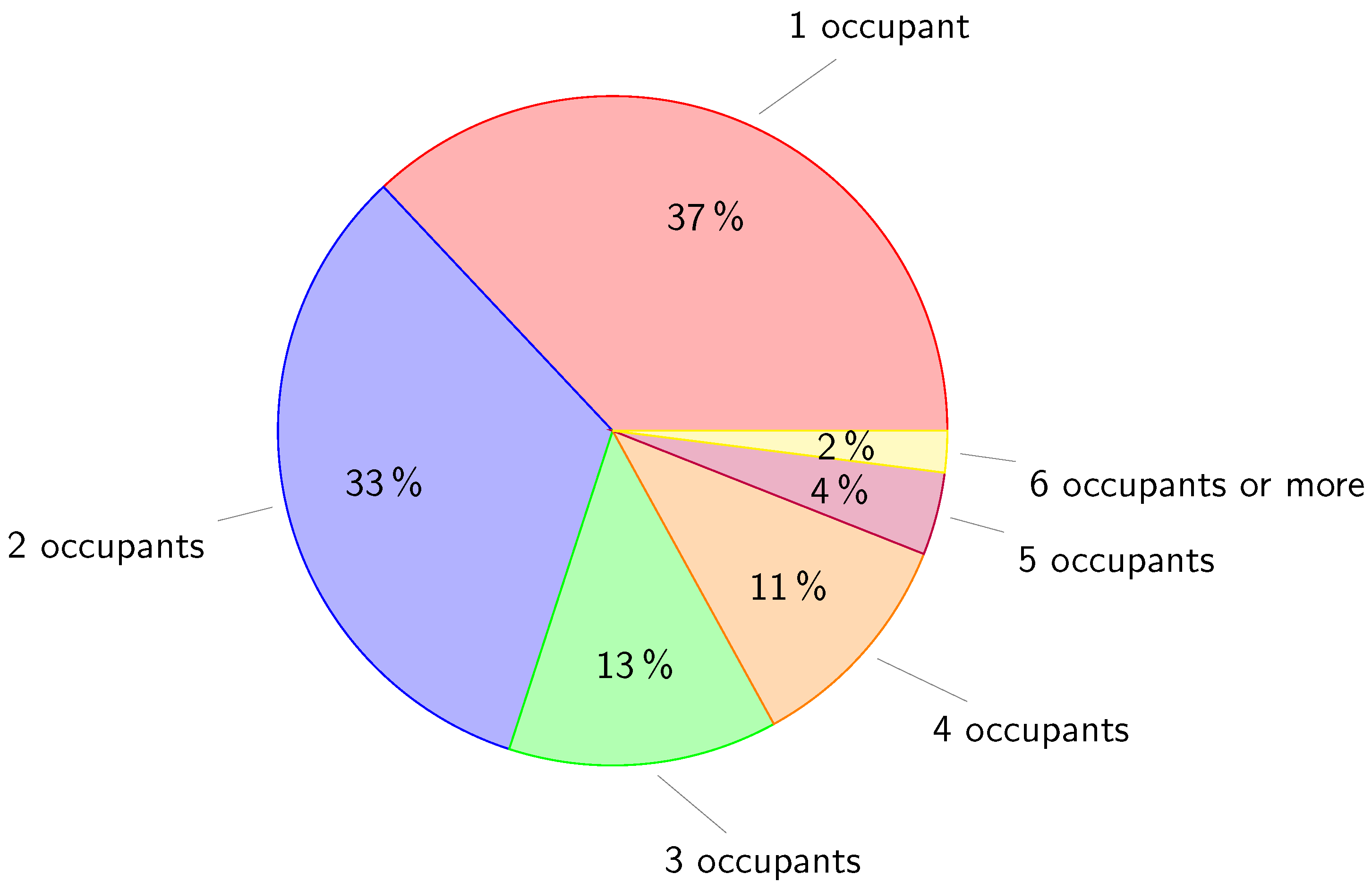
Figure 1.
Household structure in France, reported by INSEE (2021) [
55].
Figure 1.
Household structure in France, reported by INSEE (2021) [
55].
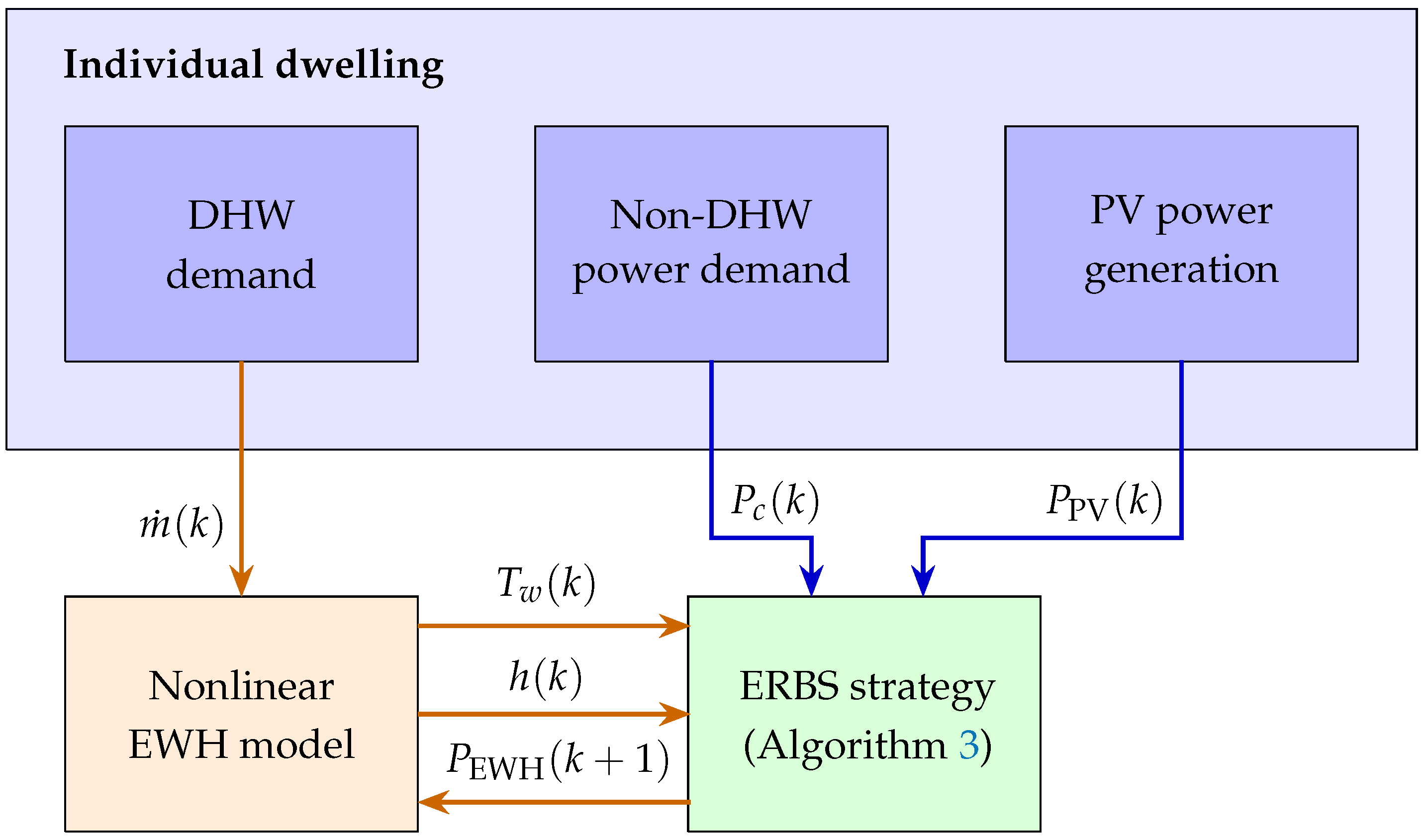
Figure 2.
Overview of the SRBS strategy. : temperature of the hot water in the tank. h: hot water height. : non-DHW power demand. : EWH heating element power. : DHW demand. SRBS: standard rule-based strategy.
Figure 2.
Overview of the SRBS strategy. : temperature of the hot water in the tank. h: hot water height. : non-DHW power demand. : EWH heating element power. : DHW demand. SRBS: standard rule-based strategy.
Figure 3.
Overview of the ERBS strategy. : temperature of the hot water in the tank. h: hot water height. : non-DHW power demand. : PV power generation. : EWH heating element power. : DHW demand. ERBS: enhanced rule-based strategy.
Figure 3.
Overview of the ERBS strategy. : temperature of the hot water in the tank. h: hot water height. : non-DHW power demand. : PV power generation. : EWH heating element power. : DHW demand. ERBS: enhanced rule-based strategy.
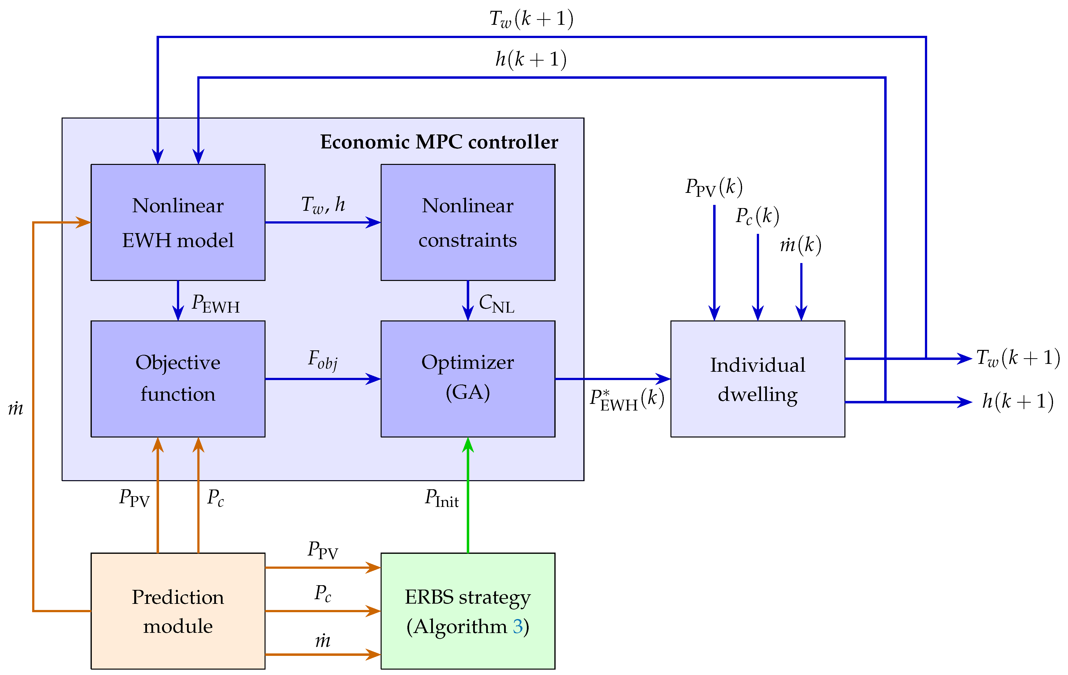
Figure 4.
Economic-model-based predictive control (MPC) scheme with a nonlinear EWH model and nonlinear constraints. : an optimized quantity. : PV power generation. : non-DHW power demand. : DHW demand. : initialization vector (EWH power vector from the ERBS strategy). : EWH heating element power. Tw: temperature of the hot water in the tank. h: hot water height. : nonlinear constraint. ERBS: enhanced rule-based strategy.
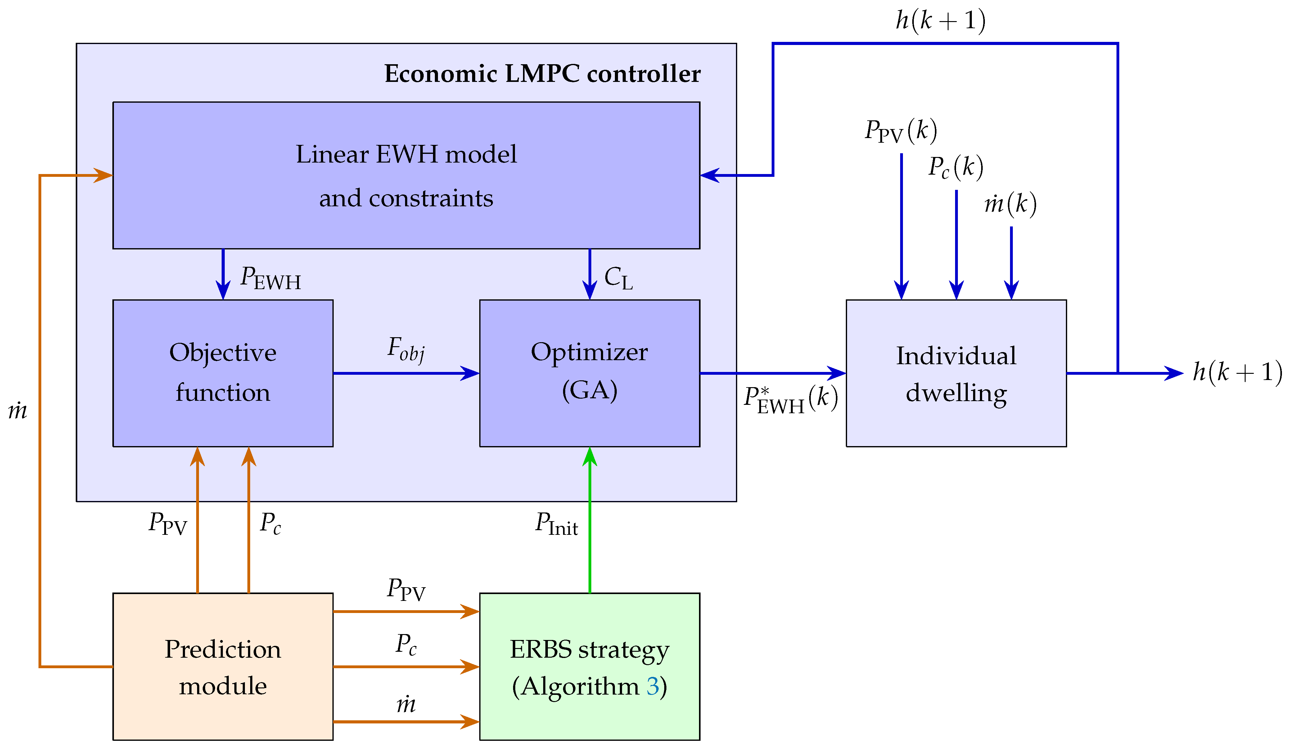
Figure 5.
Economic linear model-based predictive control (LMPC) scheme with linear EWH model and constraints. stands for an optimized quantity. : PV power generation. : non-DHW power demand. : DHW demand. : initialization vector (EWH power vector from the ERBS strategy). : EWH heating element power. h: hot water height. : linear constraint. ERBS: enhanced rule-based strategy.
Table 1.
Descriptive statistics of quantitative variable samples, where ADDDW is the approximated daily demand volume of DHW during the winter season, ADDDS is the approximated daily demand volume of DHW during the summer season, AEC is the annual electricity consumption, NUWM is the number of times per week the washing machine is used, NUCD the number of times per week the clothes dryer is used, TSFD is the total square footage of the dwelling, AgeHRP is the age of the household reference person, HHS is the household size, NYCH is the number of children under the age of 18 in the household, NOCH is the number of children over the age of 18 in the household, and NWH is the number of women over the age of 18 in the household.
| Variable | Min | Mean | Median | Max |
|---|
| ADDDW | 10 | 289.7 | 268.6 | 840 |
| ADDDS | 30 | 348.7 | 300 | 1060.7 |
| AEC | 1011 | 6001 | 5387 | 17,084 |
| NUWM | 0 | 3.261 | 3 | 10 |
| NUCD | 0 | 0.8592 | 0 | 7 |
| TSFD * | 15 | 97.72 | 95 | 250 |
| AgeHRP * | 21 | 44.74 | 44 | 82 |
| HHS * | 1 | 2.516 | 2 | 6 |
| NCH * | 0 | 0.8216 | 0 | 4 |
| NYCH | 0 | 0.108 | 0 | 2 |
| NOCH | 0 | 0.615 | 0 | 3 |
| NWH * | 0 | 1.005 | 1 | 3 |
Table 2.
Descriptive statistics of qualitative variable samples, where HS is the type of heating system, WM is the presence of a washing machine, CD is the presence of a clothes dryer, DOWD is the average daily dwelling occupancy during weekdays from 8 a.m. to 8 p.m., DOWE is the average daily dwelling occupancy during weekend days from 8 a.m. to 8 p.m., HRHBD is the habit of reducing the heating temperature in the bedrooms during the day, and HRHBN is the habit of reducing the heating temperature in the bedrooms during the night.
| Variable | Category | Frequency |
|---|
| HS | Individual (1) | 9.74% |
| Collective (2) | 88.14% |
| I do not know (3) | 2.12% |
| WM | Yes (1) | 92.80% |
| No (0) | 7.20% |
| CD * | Yes (1) | 37.29% |
| No (0) | 62.71% |
| DOWD * | Less than 4 h (1) | 47.29% |
| Between 4 and 8 h (2) | 33.90% |
| More than 8 h (2) | 18.64% |
| DOWE * | Less than 4 h (1) | 4.24% |
| Between 4 and 8 h (2) | 47.46% |
| More than 8 h (2) | 48.31% |
| HRHBD | Yes (1) | 67.37% |
| No (0) | 32.63% |
| HRHBN * | Yes (1) | 72.03% |
| No (0) | 27.97% |
Table 3.
Model parameters for the daily DHW demand in summer, where is the estimated vector of parameters, NCH is the number of children in the household, NWH is the number of women over the age of 18 in the household, AgeHRP is the age of the household reference person, TSFD is the total square footage of the dwelling, and DOWD and DOWE are the average daily dwelling occupancy during weekdays and weekend days, from 8 a.m. to 8 p.m., respectively. allows assessing the model accuracy.
| Parameter | 10% | 25% | 50% | 75% | 90% |
|---|
| 0.290 | 0.296 | 0.279 | 0.216 | 0.282 |
| 0.181 | 0.194 | 0.251 | 0.254 | 0.245 |
| −0.0010 | −0.006 | 0.002 | −0.002 | −0.004 |
| 0.002 | 0.0003 | −0.002 | −0.002 | −0.002 |
| −0.060 | −0.048 | −0.115 | −0.102 | 0.076 |
| 0.034 | −0.022 | 0.044 | 0.106 | 0.102 |
| 4.704 | 5.153 | 5.356 | 5.877 | 6.233 |
| 0.178 | 0.149 | 0.183 | 0.149 | 0.116 |
Table 4.
Model parameters for the daily DHW demand in winter, where is the estimated vector of parameters, NCH is the number of children in the household, NWH is the number of women over the age of 18 in the household, AgeHRP is the age of the household reference person, TSFD is the total square footage of the dwelling, and DOWD and DOWE are the average daily dwelling occupancy during weekdays and weekend days, from 8 a.m. to 8 p.m., respectively. allows assessing the model accuracy.
| Parameter | 10% | 25% | 50% | 75% | 90% |
|---|
| 0.195 | 0.272 | 0.290 | 0.251 | 0.177 |
| 0.219 | 0.076 | 0.230 | 0.271 | 0.233 |
| 0.001 | −0.003 | −0.004 | −0.005 | −0.010 |
| 0.003 | 0.001 | 0.0002 | −0.0001 | −0.001 |
| −0.037 | −0.103 | −0.073 | −0.132 | −0.109 |
| −0.237 | −0.066 | 0.038 | 0.037 | −0.082 |
| 4.224 | 5.006 | 5.244 | 5.691 | 6.400 |
| 0.185 | 0.154 | 0.169 | 0.173 | 0.138 |
Table 5.
Model parameters for the daily power demand, where HHS is the household size, AgeHPR is the age of household reference person, EWH is the electric water heater, TWH is the thermal water heater, SWH is the solar water heater, OWH is the other water heater, HP is the heat pump, EH is the electric heater, FH is the fire heater, RAC is the reversible air conditioning system, OH is the other heating system, CD is the clothes dryer, and HRHBN is the habit of reducing the heating temperature in the bedrooms during the night.
| Parameter | 10% | 25% | 50% | 75% | 90% |
|---|
| 0.207 | 0.188 | 0.127 | 0.160 | 0.201 |
| 0.008 | 0.011 | 0.010 | 0.009 | 0.008 |
| 0.162 | 0.346 | 0.374 | 0.183 | 0.268 |
| 0.072 | 0.343 | 0.324 | 0.133 | 0.215 |
| 0.266 | 0.212 | 0.284 | −0.030 | −0.115 |
| −0.333 | −0.263 | −0.452 | −0.179 | −0.221 |
| 0.261 | 0.267 | 0.380 | 0.346 | −0.037 |
| 0.324 | −0.029 | 0.051 | 0.218 | −0.041 |
| −0.090 | −0.274 | −0.154 | −0.100 | −0.382 |
| 0.592 | 0.292 | 0.088 | 0.201 | −0.170 |
| 0.163 | 0.062 | 0.064 | −0.007 | −0.371 |
| 0.235 | 0.271 | 0.210 | 0.197 | 0.094 |
| −0.216 | −0.144 | −0.169 | −0.184 | −0.145 |
| 4.224 | 5.006 | 5.244 | 5.691 | 6.400 |
| 0.305 | 0.267 | 0.271 | 0.247 | 0.246 |
Table 6.
Electricity purchase tariffs (
) according to EDF 2022 for contracts with on/off-peak hours over 24
[
53], in
.
Table 6.
Electricity purchase tariffs (
) according to EDF 2022 for contracts with on/off-peak hours over 24
[
53], in
.
| Period of Time | Hour Type | |
|---|
| 00 h 00–05 h 50 | Off-peak hours | 14.70 |
| 06 h 00–07 h 50 | On-peak hours | 18.41 |
| 08 h 00–11 h 50 | Off-peak hours | 14.70 |
| 12 h 00–13 h 50 | On-peak hours | 18.41 |
| 14 h 00–15 h 50 | Off-peak hours | 14.70 |
| 16 h 00–21 h 50 | On-peak hours | 18.41 |
| 22 h 00–23 h 50 | Off-peak hours | 14.70 |
Table 7.
Characteristics of the typical scenarios, where AgeHPR is the age of the reference person, NWH is the number of women over the age of 18 in the household, NCH is the number of children in the household, TSFD is the total square footage of the dwelling, and DOWD is the average daily occupancy of the dwelling during weekdays, from 8 a.m. to 8 p.m.
| Typical Scenario | 1 | 2 | 3 | 4 |
|---|
| AgeHRP | 38 | 48 | 47 | 42 |
| NWH | 1 | 1 | 1 | 1 |
| NCH | 0 | 0 | 1 | 2 |
| TSFD | 46 | 90 | 110 | 120 |
| DOWD | 2 | 3 | 5 | 6 |
Table 8.
Daily DHW demand (in
) scenarios (ADEME study and PROMES/ART-Dev study).
: ADEME daily DHW demand.
: QR daily DHW demand for the winter season.
: QR daily DHW demand for the summer season.
: normalized root mean square error relative to ground-truth values for the winter season.
: normalized root mean square error relative to ground-truth values for the summer season. See
Table 7 for the characteristics of the typical scenarios.
| Typical Scenario | 1 | 2 | 3 | 4 |
|---|
| | | | |
| 107 | 172 | 190 | 290 |
| 0.00 | 0.62 | 0.00 | 0.36 |
| 94 | 163 | 171 | 265 |
| 0.00 | 0.00 | 0.00 | 0.35 |
Table 9.
Power demand in
where
is the value from the HSS database used for validation,
is the value predicted by the HSS model, and
is the normalized root mean square error. See
Table 7 for the characteristics of the typical scenarios.
Table 9.
Power demand in
where
is the value from the HSS database used for validation,
is the value predicted by the HSS model, and
is the normalized root mean square error. See
Table 7 for the characteristics of the typical scenarios.
| Typical Scenario | 1 | 2 | 3 | 4 |
|---|
| 3881 | 4163 | 5415 | 6762 |
| 3325 | 4404 | 5298 | 6224 |
| 0.1055 | 0.0517 | 0.0251 | 0.1155 |
Table 10.
Computational cost and economic cost associated with the power extracted from the distribution grid by varying both the number of individuals and the number of generations. Configuration 1: 2000 individuals and 1000 generations. Configuration 2: 1000 individuals and 500 generations. Configuration 3: 500 individuals and 250 generations. Configuration 4: 900 individuals and 400 generations. Configurations 5: 2500 individuals and 1500 generations.
| GA Configuration | 1 | 2 | 3 | 4 | 5 |
|---|
| Computational cost | 101.60 | 60.40 | 23.90 | 38.40 | 134.20 |
| Economic cost associated with the power extracted from the distribution grid [EUR] | 3.97 | 3.96 | 3.98 | 4.01 | 3.97 |
Table 11.
GA parameters. The crossover fraction is the fraction of the population at the next generation, not including elite children, that the crossover function creates. The mutation function is the function that produces mutation children. is the optimization vector length.
Table 11.
GA parameters. The crossover fraction is the fraction of the population at the next generation, not including elite children, that the crossover function creates. The mutation function is the function that produces mutation children. is the optimization vector length.
| GA Parameter [66] | Value |
|---|
| Number of individuals | 1000 |
| Number of generations | 500 |
| Crossover function | “Laplace crossover” |
| Crossover fraction | 0.8 |
| Mutation function | “Mutation power” |
Table 12.
Mean computation time [s] for 6-day simulations, with two initialization methods.
: initialization method 1.
: initialization method 2. MPC: model-based predictive control. LMPC: linear EWH model predictive control. See
Table 7 for the characteristics of the typical scenarios.
Table 12.
Mean computation time [s] for 6-day simulations, with two initialization methods.
: initialization method 1.
: initialization method 2. MPC: model-based predictive control. LMPC: linear EWH model predictive control. See
Table 7 for the characteristics of the typical scenarios.
| Typical Scenario | Season | MPC () | MPC () | LMPC () |
|---|
| 1 | Winter | 49 | 37 | 20 |
| Spring | 42 | 17 | 21 |
| Summer | 38 | 28 | 19 |
| Autumn | 60 | 32 | 23 |
| 2 | Winter | 63 | 41 | 21 |
| Spring | 53 | 33 | 22 |
| Summer | 42 | 25 | 24 |
| Autumn | 68 | 39 | 23 |
| 3 | Winter | 52 | 34 | 19 |
| Spring | 46 | 27 | 19 |
| Summer | 34 | 20 | 16 |
| Autumn | 53 | 52 | 21 |
| 4 | Winter | 62 | 36 | 18 |
| Spring | 49 | 32 | 20 |
| Summer | 38 | 19 | 16 |
| Autumn | 70 | 42 | 31 |
Table 13.
Economic gain [EUR] for 6-day simulations (the SRBS strategy provides reference results). M
2: initialization method 2. MPC: model-based predictive control. LMPC: linear model-based predictive control. ERBS: enhanced rule-based strategy. See
Table 7 for the characteristics of the typical scenarios.
| Typical Scenario | Season | ERBS | MPC () | LMPC () |
|---|
| 1 | Winter | 0.14 | 1.00 | 0.48 |
| Spring | 0.22 | 1.00 | 0.63 |
| Summer | 0.56 | 0.85 | 0.79 |
| Autumn | 0.38 | 0.78 | 0.48 |
| 2 | Winter | 0.51 | 1.00 | 1.10 |
| Spring | 0.86 | 1.31 | 0.66 |
| Summer | 1.18 | 1.45 | 1.55 |
| Autumn | 0.66 | 1.34 | 0.74 |
| 3 | Winter | 0.37 | 0.96 | 0.50 |
| Spring | 0.80 | 1.56 | 0.90 |
| Summer | 1.08 | 1.60 | 1.50 |
| Autumn | 0.60 | 1.58 | 1.78 |
| 4 | Winter | 1.03 | 2.02 | 2.70 |
| Spring | 1.00 | 2.20 | 1.20 |
| Summer | 1.65 | 2.30 | 2.50 |
| Autumn | 1.74 | 2.20 | 1.80 |
Table 14.
Increase in the PV power generation self-consumption (SC) rate [%ps] for 6-day simulations (the SRBS strategy provides reference results). M
2: initialization method 2. MPC: model-based predictive control. LMPC: linear model-based predictive control. ERBS: enhanced rule-based strategy. See
Table 7 for the characteristics of the typical scenarios.
| Typical Scenario | Season | ERBS | MPC () | LMPC () |
|---|
| 1 | Winter | 3.00 | 13.00 | 4.80 |
| Spring | 5.00 | 11.00 | 7.80 |
| Summer | 8.00 | 10.00 | 9.60 |
| Autumn | 8.00 | 13.00 | 10.20 |
| 2 | Winter | 5.00 | 11.00 | 11.50 |
| Spring | 7.00 | 10.00 | 6.10 |
| Summer | 7.00 | 8.30 | 9.00 |
| Autumn | 9.00 | 13.00 | 9.53 |
| 3 | Winter | 3.00 | 12.00 | 5.00 |
| Spring | 6.00 | 9.00 | 6.55 |
| Summer | 7.00 | 9.00 | 7.57 |
| Autumn | 7.00 | 13.00 | 14.30 |
| 4 | Winter | 6.00 | 12.00 | 13.60 |
| Spring | 5.00 | 10.00 | 6.00 |
| Summer | 4.00 | 7.00 | 7.30 |
| Autumn | 10.00 | 13.00 | 11.00 |
Table 15.
Reduction in
emissions [
for 6-day simulations (the SRBS strategy provides reference results).
: initialization method 2. MPC: model-based predictive control. LMPC: linear model-based predictive control. ERBS: enhanced rule-based strategy. See
Table 7 for the characteristics of the typical scenarios.
| Typical Scenario | Season | ERBS | MPC () | LMPC () |
|---|
| 1 | Winter | 0.07 | 0.27 | 0.08 |
| Spring | 0.10 | 0.45 | 0.31 |
| Summer | 0.22 | 0.34 | 0.33 |
| Autumn | 0.02 | 0.32 | 0.16 |
| 2 | Winter | 0.14 | 0.19 | 0.21 |
| Spring | 0.41 | 0.67 | 0.35 |
| Summer | 0.61 | 0.74 | 0.77 |
| Autumn | 0.35 | 0.62 | 0.42 |
| 3 | Winter | 0.13 | 1.74 | 0.34 |
| Spring | 0.43 | 2.61 | 0.76 |
| Summer | 0.57 | 1.56 | 0.75 |
| Autumn | 0.37 | 0.81 | 1.23 |
| 4 | Winter | 0.16 | 0.45 | 2.68 |
| Spring | 0.45 | 3.92 | 1.01 |
| Summer | 0.69 | 1.01 | 2.25 |
| Autumn | 0.60 | 3.20 | 0.90 |


