Albedo Reflection Modeling in Bifacial Photovoltaic Modules

Abstract

This paper focuses on the analytical modeling of albedo reflection in bifacial photovoltaic modules, with particular emphasis on the backside. First, we critically examine the approaches proposed in the literature, presenting them with a tutorial style and a uniform nomenclature. These approaches are demonstrated to yield physically meaningless results, as they erroneously assume that the ground area shaded by the module acts as a source of reflected irradiance independent of the portion of sky dome visible to such an area. Then we introduce a correction based on the view factor between the shaded area and the sky. The result is a comprehensive and accurate analytical model that also describes the case of suspended panels and can be easily implemented into PV plant simulators.

1. Introduction

The rapid advancement of photovoltaic (PV) technology has led to the increasing adoption of bifacial PV modules (henceforth also referred to as panels), which are capable of capturing sunlight on both their frontside and backside (or rear). By virtue of this dual-surface capability, bifacial modules are expected to benefit from higher performance with respect to the monofacial counterparts (e.g., [1,2,3,4,5,6,7,8,9,10,11] and references therein).

One of the critical factors influencing the performance of bifacial panels is the albedo effect on the backside, i.e., the reflection of solar irradiance from the ground onto the rear surface (e.g., [12,13]). The contribution of the albedo effect to the overall energy production can be significant, especially in high-albedo environments such as snowy or sandy regions. Albedo modeling plays a crucial role in optimizing the installation parameters of bifacial modules, including tilt angle, vertical distance from the ground, as well as spacing between rows. These parameters directly affect the amount of reflected irradiance received by the rear surface and thus the overall system efficiency. A robust albedo model would help determine the optimal configuration in terms of energy production and return on investment. Without proper albedo modeling, the predicted energy yield of bifacial systems can be significantly inaccurate, leading to suboptimal designs and flawed financial assessments. For example, overestimating albedo may cause underperformance, resulting in economic losses.

The aim of this paper is twofold. First, the literature on analytical modeling of albedo reflection onto the backside of bifacial PV panels is presented in a tutorial style with a unified nomenclature to facilitate the reader’s understanding. It is found that all approaches suffer from an inconsistency leading to physically meaningless results, i.e., the irradiance reflected by the ground area shaded by the module is independent of the portion of the sky dome seen by such an area. Second, a strategy is suggested to solve this issue based on the view factor between the shaded ground and the sky. Using the proposed strategy, a comprehensive and accurate model is obtained, which allows describing the albedo reflection as a function of all the relevant parameters, namely, altitude of the Sun, tilt angle of the panel, as well as vertical distance between the panel and ground. The corrected model lends itself to easy implementation in simulation tools for the analysis of bifacial modules.

The remainder of the paper is articulated as follows: In Section 2, the literature approaches to the analytical modeling of the albedo reflection onto the rear of a bifacial panel are described and critically examined in order of growing complexity. In Section 3, the improved modeling strategy is presented, and its outcomes are reported and discussed. In Section 4, simulations of the power production of a bifacial module are conducted using an in-house tool implementing the proposed albedo model. Conclusions are then drawn in Section 5.

2. Review of the Albedo Reflection Models

In the following, we will consider a standalone infinitely-long PV module, which in three dimensions is equivalent to the practical case of a long row.

2.1. Monofacial Module

Let us denote as $G_{toth}$, $G_{bh}$, and $G_{dh}$ [W/m²] the total, beam (or direct, i.e., due to the Sun rays), and diffuse irradiances hitting the horizontal plane (or plane of horizon). $G_{toth}$ and $G_{dh}$ are available on dedicated web platforms as a function of clock time (or watch time) at chosen geographical sites for a mean day of the selected month, and $G_{bh}$ can be simply determined as the difference $G_{toth}-G_{dh}$.

As suggested in the historically relevant paper of Liu and Jordan [14] and commonly accepted since then (e.g., [15,16]), the irradiance incident on a monofacial module can be expressed as the sum of three contributions (transposition model)

$$G=G_b+G_d+G_{d,albedo}$$

(1)

where $G_b$ is the beam irradiance, $G_d$ is the diffuse irradiance from the sky, and $G_{d,albedo}$ is the diffuse irradiance reflected from the ground.

$G_b$ is given by

$$G_b=\max \left\{0,G_{bh}\cdot {\displaystyle \frac{\cos \mathsf{\theta }}{\sin \mathsf{\alpha }}}\right\}$$

(2)

where α is the solar altitude (or elevation), that is, the angle between the Sun rays and the horizontal plane (α > 0 during daytime), and θ (≥0) is the angle of incidence, i.e., the angle between the Sun rays and the normal to the panel; if θ > 90°, the Sun is behind the panel, cosθ becomes negative, and thus $G_b$ = 0 W/m² from (2).

$G_d$ is given by

$$G_d=G_{dh}\cdot F$$

(3)

where F (≤1) is the front-sky view factor. If the sky is uniformly cloudy (isotropic conditions), F is denoted as $F_i$ and is expressed as

$$F_i={\displaystyle \frac{1+\cos \mathsf{\beta }}{2}}={\cos }^2{\displaystyle \frac{\mathsf{\beta }}{2}}$$

(4)

β being the tilt (or inclination) angle of the module, i.e., the angle between the module and the horizontal plane. If the sky is clean or partially cloudy (anisotropic conditions), F is denoted as $F_a$ and accounts for mechanisms related to the position of the Sun in the sky, namely, horizon brightening and circumsolar radiation; $F_a$ can also be >1 if the panel is oriented towards the Sun. Some formulations have been proposed in the literature for $F_a$, the most recognized ones being those in [17,18].

Henceforth, let us consider modules behaving as Lambertian reflectors. $G_{d,albedo}$ is given by

$$G_{d,albedo}=G_{toth}\cdot albedo\cdot F_{albedo}$$

(5)

where albedo (<1) is a dimensionless parameter representing the ratio of the reflected upward radiation from the ground to the incident downward radiation upon it (practical values are 0.04 for fresh asphalt, 0.1–0.15 for soil ground, 0.25–0.3 for green grass, 0.4 for desert sand, 0.55 for fresh concrete, and 0.8–0.85 for freshly fallen snow), and $F_{albedo}$ (≤1) is the front-ground view factor. As the reflection from the ground is considered a Lambertian (isotropic) process, $F_{albedo}$ is expressed as

$$F_{albedo}={\displaystyle \frac{1-\cos \mathsf{\beta }}{2}}={\sin }^2{\displaystyle \frac{\mathsf{\beta }}{2}}$$

(6)

Although (6) is broadly accepted for $F_{albedo}$, it does not account for the angular losses with respect to the standard conditions, which can be included using a reduction factor [19].

The outcomes of (6) in the entire range of practical β values, namely, from β = 0° (horizontal panel) to β = 90° (vertically deployed panel) are reasonable: $F_{albedo}$ = 0 if β = 0° since the panel front does not see the ground (it only sees the sky); $F_{albedo}$ increases with β and is eventually equal to 0.5 as β = 90° since the front sees half ground.

It is worth noting that under isotropic conditions the sum of the front-sky and front-ground view factors is 1, that is,

$$F_i+F_{albedo}=1$$

(7)

2.2. Bifacial Module: Albedo Reflection onto the Rear Without Self-Shading

Formulations (1)–(6) can be safely applied to the frontside of a bifacial module as β still falls in the range 0° to 90°.

For the backside of the module, the following considerations are in order. The tilt and incidence angles of the rear are the supplement of the corresponding angles associated with the front

$${\mathsf{\beta }}_{rear}=180°-\mathsf{\beta }$$

(8)

$${\mathsf{\theta }}_{rear}=180°-\mathsf{\theta }$$

(9)

An illustrative representation of all angles is provided in Figure 1.

The irradiance landing on the rear can be expressed as

$$G_{rear}=G_{b,rear}+G_{d,rear}+G_{d,albedo,rear}$$

(10)

where $G_{b,rear}$ is the beam irradiance, $G_{d,rear}$ is the diffuse irradiance from the sky, and $G_{d,albedo,rear}$ is the diffuse irradiance reflected from the ground.

$G_{b,rear}$ is given by

$$G_{b,rear}=\max \left\{0,G_{bh}\cdot {\displaystyle \frac{\cos {\mathsf{\theta }}_{rear}}{\sin \mathsf{\alpha }}}\right\}=\max \left\{0,-G_{bh}\cdot {\displaystyle \frac{\cos \mathsf{\theta }}{\sin \mathsf{\alpha }}}\right\}$$

(11)

$G_{d,rear}$ is given by

$$G_{d,rear}=G_{dh}\cdot F_{rear}$$

(12)

Under isotropic conditions, the rear-sky view factor $F_{rear}$ (≤1) is denoted as $F_{i,rear}$ and is given by

$$F_{i,rear}={\displaystyle \frac{1+\cos {\mathsf{\beta }}_{rear}}{2}}={\cos }^2{\displaystyle \frac{{\mathsf{\beta }}_{rear}}{2}}={\displaystyle \frac{1-\cos \mathsf{\beta }}{2}}={\sin }^2{\displaystyle \frac{\mathsf{\beta }}{2}}$$

(13)

Under anisotropic conditions, $F_{rear}$ is denoted as $F_{a,rear}$, for which it is possible to use formulations like those in [17,18] by replacing β and θ with ${\mathsf{\beta }}_{rear}$ and ${\mathsf{\theta }}_{rear}$, respectively.

While the first and second terms on the right-hand side of (10) are straightforwardly obtained from the corresponding counterparts in (1), the third contribution $G_{d,albedo,rear}$ due to the albedo reflection from the ground to the rear deserves higher attention. Inspired by (5) and (6), one might erroneously express $G_{d,albedo,rear}$ as

$$G_{d,albedo,rear}=G_{toth}\cdot albedo\cdot F_{albedo,rear}$$

(14)

with the rear-ground view factor $F_{albedo,rear}$ (≤1) given by [20,21]

$$F_{albedo,rear}={\displaystyle \frac{1-\cos {\mathsf{\beta }}_{rear}}{2}}={\sin }^2{\displaystyle \frac{{\mathsf{\beta }}_{rear}}{2}}={\displaystyle \frac{1+\cos \mathsf{\beta }}{2}}={\cos }^2{\displaystyle \frac{\mathsf{\beta }}{2}}$$

(15)

Unfortunately, differently from (5) and (6), (14) and (15) do not provide physically meaningful results within the range of practical β values. If β is lowered from 90° to 0°, $F_{albedo,rear}$ increases, eventually becoming 1 for β = 0° (horizontal panel with the frontside oriented towards the sky and backside lying on the ground); consequently, $G_{d,albedo,rear}$ incorrectly increases as β decreases, and reaches its maximum value for β = 0° when instead it should be 0 W/m² as the ground beneath the flat panel cannot reflect sunlight. This is the consequence of the incorrectness of (14), which assumes that the ground reflects an irradiance given by $G_{toth}\cdot albedo$ independently of the inclination of the module and thus of the sky dome visible to the ground. Additionally, similarly to (5) and (6), (14) and (15) do not account for the shadow cast by the module itself onto the ground (self-shading) and do not include the dependence upon the vertical distance d between the lowest module edge and the ground, which is expected to play a key role.

2.3. Cross-String Rule

As shown earlier, view factors are of utmost importance in the context of PV systems, as they permeate the mathematical basis for assessing irradiance on module surfaces. Since the following sections will address more complex geometrical scenarios, before proceeding, we will briefly recall the well-established cross-string rule, which allows for a straightforward determination of view factors [9,20,22,23]. By considering the infinitely-long surfaces A and B in Figure 2, the view factors $F_{A-B}$ and $F_{B-A}$ can be calculated as

$$F_{A-B}={\displaystyle \frac{\overline{CF}+\overline{DE}-\overline{CE}-\overline{DF}}{2\cdot \overline{CD}}}$$

(16)

$$F_{B-A}={\displaystyle \frac{\overline{CF}+\overline{DE}-\overline{CE}-\overline{DF}}{2\cdot \overline{EF}}}$$

(17)

where $\overline{CD}$ and $\overline{EF}$ are the heights of A and B, respectively, $\overline{DE}$ and $\overline{CF}$ are the diagonals between the borders, $\overline{CE}$ and $\overline{DF}$ are the distances between the surface edges.

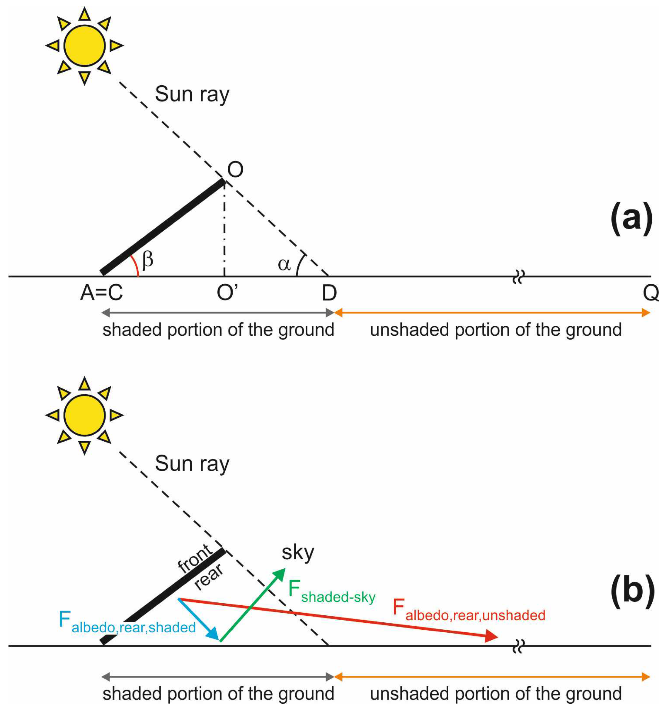
2.4. Bifacial Module: Albedo Reflection onto the Rear with Self-Shading

The standard approach to account for the self-shading is to express $G_{d,albedo,rear}$ as [6,9,20,24,25,26]

$$G_{d,albedo,rear}=G_{toth}\cdot albedo\cdot F_{albedo,rear,unshaded}+G_{dh}\cdot albedo\cdot F_{albedo,rear,shaded}$$

(18)

where $F_{albedo,rear,unshaded}$ is the view factor between rear and unshaded ground, and $F_{albedo,rear,shaded}$ is the view factor between rear and ground shaded by the panel; both view factors are illustratively represented in Figure 3. In [20], Appelbaum determines such view factors for the case d = 0 m (the lowest panel edge is in contact with the ground) by resorting to the cross-string rule. Here, we revisit the calculations, achieving clearer and more easily implementable formulations. Let us denote the height of the module as H_panel. With reference to Figure 3, $F_{albedo,rear,unshaded}$ can be evaluated as

$$\begin{array}{cc}\hfill F_{albedo,rear,unshaded}& =F_{rear-DQ}=F_{AO-DQ}=\hfill \\ & ={\displaystyle \frac{\overline{AQ}+\overline{OD}-\overline{AD}-\overline{OQ}}{2\cdot \overline{AO}}}={\displaystyle \frac{\left(\overline{AQ}-\overline{OQ}\right)+\overline{OD}-\overline{AD}}{2\cdot \overline{AO}}}\approx {\displaystyle \frac{\overline{A{O}^{\prime }}+\overline{OD}-\overline{AD}}{2\cdot \overline{AO}}}\hfill \end{array}$$

(19)

as Q is a point very far away from the panel. In (19),

$$\overline{AO}=H_{panel},\overline{A{O}^{\prime }}=H_{panel}\cdot \cos \mathsf{\beta },\overline{OD}={\displaystyle \frac{\overline{O{O}^{\prime }}}{\sin \mathsf{\alpha }}}={\displaystyle \frac{H_{panel}\cdot \sin \mathsf{\beta }}{\sin \mathsf{\alpha }}},$$

and $\overline{AD}=\overline{A{O}^{\prime }}+\overline{O^{\prime }D}=H_{panel}\cdot \cos \mathsf{\beta }+\overline{OD}\cdot \cos \mathsf{\alpha }=H_{panel}\cdot \left(\cos \mathsf{\beta }+{\displaystyle \frac{\sin \mathsf{\beta }}{\tan \mathsf{\alpha }}}\right)$.

By substituting into (19),

$$\begin{array}{cc}\hfill F_{albedo,rear,unshaded}& ={\displaystyle \frac{H_{panel}\cdot \cos \mathsf{\beta }+\frac{H_{panel}\cdot \sin \mathsf{\beta }}{\sin \mathsf{\alpha }}-H_{panel}\cdot \left(\cos \mathsf{\beta }+\frac{\sin \mathsf{\beta }}{\tan \mathsf{\alpha }}\right)}{2\cdot H_{panel}}}=\hfill \\ & ={\displaystyle \frac{\sin \mathsf{\beta }}{2}}\cdot \left({\displaystyle \frac{1}{\sin \mathsf{\alpha }}}-{\displaystyle \frac{1}{\tan \mathsf{\alpha }}}\right)={\displaystyle \frac{\sin \mathsf{\beta }}{2}}\cdot {\displaystyle \frac{1-\cos \mathsf{\alpha }}{\sin \mathsf{\alpha }}}\hfill \end{array}$$

(20)

$F_{albedo,rear,shaded}$ can be determined as

$$\begin{array}{cc}\hfill F_{albedo,rear,shaded}& =F_{rear-CD}=F_{AO-CD}={\displaystyle \frac{\overline{OC}+\overline{AD}-\overline{AC}-\overline{OD}}{2\cdot \overline{AO}}}={\displaystyle \frac{\overline{OC}+\overline{AD}-\overline{OD}}{2\cdot \overline{AO}}}=\hfill \\ & ={\displaystyle \frac{H_{panel}+H_{panel}\cdot \left(\cos \mathsf{\beta }+\frac{\sin \mathsf{\beta }}{\tan \mathsf{\alpha }}\right)-\frac{H_{panel}\cdot \sin \mathsf{\beta }}{\sin \mathsf{\alpha }}}{2\cdot H_{panel}}}=\hfill \\ & ={\displaystyle \frac{1+\cos \mathsf{\beta }}{2}}-{\displaystyle \frac{\sin \mathsf{\beta }}{2}}\cdot {\displaystyle \frac{1-\cos \mathsf{\alpha }}{\sin \mathsf{\alpha }}}\hfill \end{array}$$

(21)

As a proof of the correctness of the derivation, the sum of the rear-sky view factor (13), the view factor between rear and unshaded ground (20), and the view factor between rear and shaded ground (21) gives 1.

Figure 4 shows the view factors given by (20) and (21) in the practical β range. For β = 90°, the sum of the view factors is 0.5 as the backside sees half ground; as β is lowered, $F_{albedo,rear,unshaded}$ reduces and $F_{albedo,rear,shaded}$ increases, eventually tending to 0 and 1, respectively, as the backside intimately sees only the shaded portion of the ground. Hence, model (18) provides unreasonable results since $G_{dh}\cdot albedo\cdot F_{albedo,rear,shaded}$ incorrectly increases with decreasing β and tends to its maximum value for β = 0°, when it is expected to be 0 W/m² since the backside lies flat on the ground. Again, this is due to the inconsistency of such a term, which inherently assumes that the shaded ground reflects an irradiance given by $G_{dh}\cdot albedo$, independently of the inclination of the module, and thus of the sky dome seen by the shaded area. Furthermore, such a model is still limited to the case d = 0 m, which does not allow describing the case of suspended PV fields.

In [26], Gu and his coauthors extend Appelbaum’s approach by including the case of a suspended panel (d > 0) in the derivation of $F_{albedo,rear,unshaded}$ and $F_{albedo,rear,shaded}$ to be used in (18). Again, we reexamine the calculations with the aim of expressing the resulting formulations in an easier-to-use way. With reference to Figure 5, where the same nomenclature in [26] is adopted for the sake of simplicity, the view factor $F_{albedo,rear,unshaded}$ is given by the sum of two contributions

$$F_{albedo,rear,unshaded}=F_{albedo,rear,unshaded1}+F_{albedo,rear,unshaded2}=F_{rear-DQ}+F_{rear-FC}=F_{AO-DQ}+F_{AO-FC}$$

(22)

where, analogously to (19),

$$F_{AO-DQ}={\displaystyle \frac{\overline{AQ}+\overline{OD}-\overline{AD}-\overline{OQ}}{2\cdot \overline{AO}}}={\displaystyle \frac{\left(\overline{AQ}-\overline{OQ}\right)+\overline{OD}-\overline{AD}}{2\cdot \overline{AO}}}\approx {\displaystyle \frac{\overline{A{O}^{\prime }}+\overline{OD}-\overline{AD}}{2\cdot \overline{AO}}}$$

(23)

Here, $\overline{AO}=H_{panel}$, $\overline{A{O}^{\prime }}=H_{panel}\cdot \cos \mathsf{\beta }$,

$$\overline{OD}={\displaystyle \frac{\overline{O{O}^{″}}}{\sin \mathsf{\alpha }}}={\displaystyle \frac{\overline{O{O}^{\prime }}+d}{\sin \mathsf{\alpha }}}={\displaystyle \frac{H_{panel}\cdot \sin \mathsf{\beta }}{\sin \mathsf{\alpha }}}+{\displaystyle \frac{d}{\sin \mathsf{\alpha }}},$$

$\overline{AD}=\sqrt{{\overline{BD}}^2+d^2}$, where

$$\overline{BD}=\overline{B{O}^{″}}+\overline{O^{″}D}=\overline{A{O}^{\prime }}+\overline{OD}\cdot \cos \mathsf{\alpha }=H_{panel}\cdot \cos \mathsf{\beta }+{\displaystyle \frac{H_{panel}\cdot \sin \mathsf{\beta }}{\tan \mathsf{\alpha }}}+{\displaystyle \frac{d}{\tan \mathsf{\alpha }}}$$

By substituting into (23),

$$F_{AO-DQ}={\displaystyle \frac{H_{panel}\cdot \cos \mathsf{\beta }+\frac{H_{panel}\cdot \sin \mathsf{\beta }}{\sin \mathsf{\alpha }}+\frac{d}{\sin \mathsf{\alpha }}-\sqrt{{\left(H_{panel}\cdot \cos \mathsf{\beta }+\frac{H_{panel}\cdot \sin \mathsf{\beta }}{\tan \mathsf{\alpha }}+\frac{d}{\tan \mathsf{\alpha }}\right)}^2+d^2}}{2\cdot H_{panel}}}$$

(24)

which for d = 0 m reduces to (20). The second term on the right-hand side of (22) is given by

$$F_{AO-FC}={\displaystyle \frac{\overline{OF}+\overline{AC}-\overline{AF}-\overline{OC}}{2\cdot \overline{AO}}}$$

(25)

where $\overline{AC}={\displaystyle \frac{d}{\sin \mathsf{\alpha }}}$, $\overline{AF}={\displaystyle \frac{d}{\sin \mathsf{\beta }}}$, $\overline{OF}=\overline{AO}+\overline{AF}=H_{panel}+{\displaystyle \frac{d}{\sin \mathsf{\beta }}}$,

$$\begin{array}{cc}\hfill \overline{OC}& =\sqrt{{\overline{O{O}^{″}}}^2+{\overline{C{O}^{″}}}^2}=\sqrt{{\left(H_{panel}\cdot \sin \mathsf{\beta }+d\right)}^2+{\left(\overline{B{O}^{″}}-\overline{BC}\right)}^2}=\hfill \\ & =\sqrt{{\left(H_{panel}\cdot \sin \mathsf{\beta }+d\right)}^2+{\left(H_{panel}\cdot \cos \mathsf{\beta }-{\displaystyle \frac{d}{\tan \mathsf{\alpha }}}\right)}^2}\hfill \end{array}$$

By substituting into (25), it is obtained that

$$F_{AO-FC}={\displaystyle \frac{H_{panel}+\frac{d}{\sin \mathsf{\alpha }}-\sqrt{{\left(H_{panel}\cdot \sin \mathsf{\beta }+d\right)}^2+{\left(H_{panel}\cdot \cos \mathsf{\beta }-\frac{d}{\tan \mathsf{\alpha }}\right)}^2}}{2\cdot H_{panel}}}$$

(26)

which for d = 0 m reduces to 0.

The view factor $F_{albedo,rear,shaded}$ is expressed as

$$F_{albedo,rear,shaded}=F_{rear-CD}=F_{AO-CD}={\displaystyle \frac{\overline{OC}+\overline{AD}-\overline{AC}-\overline{OD}}{2\cdot \overline{AO}}}$$

(27)

By substituting all the previously evaluated terms into (27) and rearranging,

$$\begin{array}{l}{F}_{albedo,rear,shaded}=\\ ={\displaystyle \frac{\sqrt{{\left(H_{panel}\cdot \sin \mathsf{\beta }+d\right)}^2+{\left(H_{panel}\cdot \cos \mathsf{\beta }-\frac{d}{\tan \mathsf{\alpha }}\right)}^2}+\sqrt{{\left(H_{panel}\cdot \cos \mathsf{\beta }+\frac{H_{panel}\cdot \sin \mathsf{\beta }}{\tan \mathsf{\alpha }}+\frac{d}{\tan \mathsf{\alpha }}\right)}^2+d^2}-\frac{2d}{\sin \mathsf{\alpha }}-\frac{H_{panel}\cdot \sin \mathsf{\beta }}{\sin \mathsf{\alpha }}}{2\cdot H_{panel}}}\end{array}$$

(28)

which for d = 0 m reduces to (21).

Figure 6 reports the behavior of $F_{albedo,rear,unshaded}$ according to (22) with (24), (26), and $F_{albedo,rear,shaded}$ given by (28) as a function of distance d for various tilt angles β, considering H_panel = 0.719 m and α = 40°. It is worth noting that, for β = 0° (horizontal panel), the sum of the view factors from rear to ground is equal to 1 regardless of d, as the rear only sees the ground; for β = 30° such a sum is 0.933, while, for β = 90° (vertical panel) it amounts to 0.5 as the rear sees half ground. $F_{albedo,rear,shaded}$ reduces with growing d, whereas $F_{albedo,rear,unshaded}$ increases, as the farther the suspended panel is from ground, the smaller the percentage of shaded area seen by the backside.

Although the rear-ground view factors $F_{albedo,rear,unshaded}$ and $F_{albedo,rear,shaded}$ are correctly described as a function of β and d, model (18) for $G_{d,albedo,rear}$ is still physically meaningless since the term $G_{dh}\cdot albedo\cdot F_{albedo,rear,shaded}$ assumes that the shaded ground is a source of irradiance $G_{dh}\cdot albedo$, independently of β and d, and thus of the portion of sky dome seen by the shaded ground. Therefore, it can once again be concluded that the mere multiplication by the view factor between rear and ground $F_{albedo,rear,shaded}$ is insufficient to model the albedo reflection produced by the shaded ground.

Table 1. Characteristics and limitations of the available analytical models for the diffuse irradiance impinging on the panel rear due to the albedo reflection from the ground (G_{d,albedo,rear}).

Gd,albedo,rear Models	Characteristics and Limitations
model (14) using (15)	It neglects the self-shading, assuming that the whole ground is irradiated It inherently assumes that the lower edge of the module is in contact with the ground, i.e., the case of suspended modules is not covered The irradiance increases when decreasing the tilt angle of the panel β, which is physically meaningless, and reaches the maximum value for β = 0° (backside horizontally lying on the ground) when it is expected to be 0°W/m2
model (18) using (20) and (21)	It accounts for the self-shading, by partitioning the ground into an unshaded region and an area shaded by the module itself It assumes that the lower edge of the module is in contact with the ground, i.e., the case of suspended modules is not covered The irradiance reflected from the shaded portion of the ground is independent of the tilt angle of the panel β and thus of the portion of the sky dome visible to the shaded ground; consequently, such an irradiance erroneously increases as β reduces, eventually reaching the maximum value for β = 0° when it must be 0°W/m2
model (18) using (22) with (24), (26), and (28)	It accounts for the self-shading The lower edge of the module is at an arbitrary vertical distance from the ground d, that is, the case of suspended modules is considered The irradiance reflected from the shaded ground area is independent of β and d, and therefore of the portion of the sky dome visible to the shaded ground

provides a comprehensive and clear overview of characteristics and limitations of the examined analytical models for $G_{d,albedo,rear}$.

3. Our Approach

We propose an improved version of (18) given by

$$G_{d,albedo,rear}=G_{toth}\cdot albedo\cdot F_{albedo,rear,unshaded}+G_{dh}\cdot F_{shaded-sky}\cdot albedo\cdot F_{albedo,rear,shaded}$$

(29)

where $F_{shaded-sky}$ is the view factor between shaded ground and sky, the illustrative representation of which is shown in Figure 3b and Figure 5b. Formulation (22) using (24), (26), which reduces to (20) for d = 0 m, can be applied to $F_{albedo,rear,unshaded}$, and formulation (28), which reduces to (21) for d = 0 m, can be adopted for $F_{albedo,rear,shaded}$. In (29), the diffuse irradiance actually landing on the area shaded by the module is not merely $G_{dh}$ as in (18) but is more properly given by $G_{dh}\cdot F_{shaded-sky}$ since $G_{dh}$ must be weighted by the portion of the sky dome seen by the shaded area of the ground.

Here, we first evaluate $F_{shaded-sky}$ for the case d = 0 m; with reference to Figure 3,

$$\begin{array}{cc}\hfill F_{shaded-sky}& =F_{CD-OD}={\displaystyle \frac{\overline{CD}+\overline{OD}-\overline{CO}}{2\cdot \overline{CD}}}={\displaystyle \frac{\overline{AD}+\overline{OD}-\overline{AO}}{2\cdot \overline{AD}}}=\hfill \\ & ={\displaystyle \frac{H_{panel}\cdot \left(\cos \mathsf{\beta }+\frac{\sin \mathsf{\beta }}{\tan \mathsf{\alpha }}\right)+H_{panel}\cdot \frac{\sin \mathsf{\beta }}{\sin \mathsf{\alpha }}-H_{panel}}{2\cdot H_{panel}\cdot \left(\cos \mathsf{\beta }+\frac{\sin \mathsf{\beta }}{\tan \mathsf{\alpha }}\right)}}={\displaystyle \frac{\cos \mathsf{\beta }+\sin \mathsf{\beta }\cdot \frac{1+\cos \mathsf{\alpha }}{\sin \mathsf{\alpha }}-1}{2\cdot \left(\cos \mathsf{\beta }+\frac{\sin \mathsf{\beta }}{\tan \mathsf{\alpha }}\right)}}\hfill \end{array}$$

(30)

For an arbitrary d, with reference to Figure 5,

$$F_{shaded-sky}=F_{shaded-sky1}+F_{shaded-sky2}=F_{CD-OD}+F_{CD-FA}$$

(31)

$F_{CD-OD}$ is given by

$$F_{CD-OD}={\displaystyle \frac{\overline{CD}+\overline{OD}-\overline{CO}}{2\cdot \overline{CD}}}$$

(32)

where $\overline{CD}=\overline{BD}-\overline{BC}=H_{panel}\cdot \cos \mathsf{\beta }+{\displaystyle \frac{H_{panel}\cdot \sin \mathsf{\beta }}{\tan \mathsf{\alpha }}}+{\displaystyle \frac{d}{\tan \mathsf{\alpha }}}-{\displaystyle \frac{d}{\tan \mathsf{\alpha }}}=H_{panel}\cdot \left(\cos \mathsf{\beta }+{\displaystyle \frac{\sin \mathsf{\beta }}{\tan \mathsf{\alpha }}}\right)$ and $\overline{OD}$, $\overline{CO}=\overline{OC}$ were evaluated earlier. By substituting into (32),

$$F_{CD-OD}={\displaystyle \frac{H_{panel}\cdot \left(\cos \mathsf{\beta }+\frac{\sin \mathsf{\beta }}{\tan \mathsf{\alpha }}\right)+\frac{H_{panel}\cdot \sin \mathsf{\beta }}{\sin \mathsf{\alpha }}+\frac{d}{\sin \mathsf{\alpha }}-\sqrt{{\left(H_{panel}\cdot \sin \mathsf{\beta }+d\right)}^2+{\left(H_{panel}\cdot \cos \mathsf{\beta }-\frac{d}{\tan \mathsf{\alpha }}\right)}^2}}{2\cdot H_{panel}\cdot \left(\cos \mathsf{\beta }+\frac{\sin \mathsf{\beta }}{\tan \mathsf{\alpha }}\right)}}$$

(33)

which for d = 0 m reduces to (30).

$F_{CD-FA}$ is given by

$$F_{CD-FA}={\displaystyle \frac{\overline{CA}+\overline{DF}-\overline{FC}-\overline{AD}}{2\cdot \overline{CD}}}={\displaystyle \frac{\overline{AC}+\overline{CD}-\overline{AD}}{2\cdot \overline{CD}}}$$

(34)

where $\overline{AC}$, $\overline{CD}$, and $\overline{AD}$ were determined before. By substituting into (34),

$$F_{CD-FA}={\displaystyle \frac{\frac{d}{\sin \mathsf{\alpha }}+H_{panel}\cdot \left(\cos \mathsf{\beta }+\frac{\sin \mathsf{\beta }}{\tan \mathsf{\alpha }}\right)-\sqrt{{\left(H_{panel}\cdot \cos \mathsf{\beta }+\frac{H_{panel}\cdot \sin \mathsf{\beta }}{\tan \mathsf{\alpha }}+\frac{d}{\tan \mathsf{\alpha }}\right)}^2+d^2}}{2\cdot H_{panel}\cdot \left(\cos \mathsf{\beta }+\frac{\sin \mathsf{\beta }}{\tan \mathsf{\alpha }}\right)}}$$

(35)

which for d = 0 m reduces to 0.

Figure 7 shows $F_{shaded-sky}$ vs. tilt angle β for d = 0 m (keeping α = 40°) and vs. distance d for various β values (α = 40° and H_panel = 0.719 m). It can be inferred that for d = 0 m $F_{shaded-sky}$ decreases with reducing β as the shaded area produced by the module sees a lower portion of the sky dome and eventually becomes 0 if β = 0°, as the shaded area is covered by the flat module and cannot see the sky; in addition, $F_{shaded-sky}$ reasonably increases with d for a given β: the farther the module is from the ground, the more sky is seen by the shaded area.

Figure 8 demonstrates the physical validity of our approach. More specifically, such a figure shows the behavior of the 1st and 2nd terms on the right-hand side of (29), namely, $G_{toth}\cdot albedo\cdot F_{albedo,rear,unshaded}$ and $G_{dh}\cdot F_{shaded-sky}\cdot albedo\cdot F_{albedo,rear,shaded}$, respectively, by varying β for $G_{toth}$ = 700 W/m², $G_{dh}$ = 200 W/m², albedo = 0.5, d = 0 m, so that $F_{shaded-sky}$ reduces to (30), and α = 40°. As can be seen, if β = 0°, both contributions are equal to 0 W/m² as the backside entirely lies on the ground, so that $F_{albedo,rear,unshaded}=0$, and, despite $F_{albedo,rear,shaded}=1$, the 2nd term $G_{dh}\cdot F_{shaded-sky}\cdot albedo\cdot F_{albedo,rear,shaded}$ is equal to 0 since the shaded area of the ground does not see the sky ($F_{shaded-sky}=0$). The 1st term $G_{toth}\cdot albedo\cdot F_{albedo,rear,unshaded}$ obviously increases with β since the rear sees more and more unshaded ground; interestingly, the 2nd term $G_{dh}\cdot F_{shaded-sky}\cdot albedo\cdot F_{albedo,rear,shaded}$ initially increases since the fast growth in $F_{shaded-sky}$ for low β values (Figure 7a) prevails over the reduction in $F_{albedo,rear,shaded}$ (Figure 4), reaches a maximum around β = 45° and then decreases since for high β values the increase in $F_{shaded-sky}$ is slower, and the reduction in $F_{albedo,rear,shaded}$ dominates. Also shown in Figure 8 is the meaningless behavior—and the significant irradiance overestimation—that would be obtained by using the 2nd term $G_{dh}\cdot albedo\cdot F_{albedo,rear,shaded}$ on the right-hand side of (18).

Concerning the frontside, (5) and (6) can be considered accurate enough for low β values; on the other hand, if β is high, e.g., for vertical panels, the albedo reflection should be accounted for with the same approach as in Section 3.

4. Impact on Power Production

In order to estimate the beneficial impact of the improved model (29) with $F_{shaded-sky}$ given by (31) using (33) and (35), we implemented such a model in an advanced version of an in-house tool, originally designed for the analysis and optimization of monofacial PV modules [27] and recently extended to bifacial ones [28].

The tool benefits from a high-granularity cell level discretization, and it is fed with the following information:

• The latitude ϕ and the local longitude λ, denoted as λ_local, of the geographical site where the PV module is installed.
• The longitude λ_standard of the standard meridian on which the clock time (CKT, also referred to as watch time or standard local time) is based.
• The day of the year n.
• The azimuth angle of the module front γ.
• The tilt angle of the module front β.
• The distance d between the lower edge of the module and ground.
• The albedo value.
• The total and diffuse irradiances $G_{toth}$ and $G_{dh}$ hitting the horizontal plane, as well as the ambient temperature $T_{amb}$ as a function of CKT at the selected geographical site. For the simulations performed in this section, these data were taken from the PhotoVoltaic Geographical Information System (PVGIS) website [29]; here, it is stated that they were evaluated for the mean day of the chosen month from satellite data through a sophisticated algorithm accounting for sky obstruction (shading) due to local terrain features (hills or mountains) calculated from a digital elevation model.
• Some key parameters available in the module datasheet, namely, the nominal operating cell temperature $T_{NOCT}$, the short-circuit current under nominal conditions $I_{scnom}$, and the percentage temperature coefficient of the short-circuit current $I_{sc}$.

The tool evaluates:

• The total irradiances on the front (G) and rear ($G_{rear}$), the operating temperature of the cells (T), as well as the currents photogenerated by the front ($I_{ph}$) and rear ($I_{ph,rear}$) vs. CKT under isotropic and anisotropic sky conditions.
• The I–V characteristic of the module–and consequently the maximum produced power $P_{max}$–at each CKT during the day.

The individual cells are described with an enriched variant of the model presented in [30,31,32], which accounts for series and shunt resistances, the increase in the reverse current due to the avalanche mechanism, as well as for the temperature dependence of the temperature-sensitive parameters. The entire tool is developed as a Matlab code. If the cells of the module do not share the same parameters or the same irradiances and temperature (nonuniform cell behavior), Matlab invokes OrCAD PSPICE [33] to compute the I–V characteristic at a given daytime CKT.

The site selected as a case-study was Naples (ϕ = 40°50′, λ_local = 14°15′, λ_standard = 15°). A bifacial silicon module, embedding 40 cells and subdivided into two 20-cell subpanels, was oriented to South (γ = 0°), tilted with β = 30°, and assumed in contact with the ground (d = 0 m), the albedo of which was considered equal to 0.5. The simulation analysis was performed over two days, namely, July 15 (n = 196) and October 15 (n = 288) under daylight-saving conditions. The results were compared with those obtained using the inaccurate (18) that assumes the shaded ground as a source of constant irradiance $G_{dh}\cdot albedo$.

Figure 9 shows the maximum power normalized to the peak power provided on the datasheet as a function of clock time CKT for both days. As can be seen, exploiting the widely used (18) leads to a perceptible overestimation of the performance of the panel, ranging within 6% to 9% on July 15 and 4.5% to 5.5% on October 15. This could result in a significant inaccuracy in the predicted yearly energy yield and lead to an undersized system design, eventually causing economic losses.

5. Conclusions

In this paper, we have conducted a comprehensive review of the analytical modeling of the albedo reflection onto the rear of bifacial photovoltaic (PV) modules. This review has highlighted a critical limitation of the widely diffused approaches, i.e., the assumption that the self-shaded ground contributes a reflected irradiance merely given by the product between the horizontal diffuse irradiance and albedo, without considering the portion of the sky dome seen by the shaded area. This simplification may lead to a marked irradiance overestimation, especially in high-albedo environments.

To tackle and solve this issue, we have introduced a correction based on the view factor between the ground shaded by the panel and the sky. This adjustment ensures an accurate modeling of the interplay between self-shading and irradiance reflection. The corrected model accounts for altitude of the Sun, inclination of the module, and vertical distance between the lowest edge of the module and ground. The model has been easily implemented in an in-house simulation tool designed to evaluate the energy production of bifacial PV plants. Results have provided evidence that the proposed approach effectively prevents yield overestimations that would arise from traditional methods, thus mitigating the risk of developing underrated PV systems. Hence, it can be suggested for inclusion in commercial and custom simulation programs for academic and industry applications.

References

1. Guo, S.; Walsh, T.M.; Peters, M. Vertically mounted bifacial photovoltaic modules: A global analysis. Energy 2013, 61, 447–454. [Google Scholar] [CrossRef]
2. Appelbaum, J. Bifacial photovoltaic panels field. Renew. Energy 2016, 85, 338–343. [Google Scholar] [CrossRef]
3. Guerrero-Lemus, R.; Vega, R.; Kim, T.; Kimm, A.; Shephard, L.E. Bifacial solar photovoltaics—A technology review. Renew. Sustain. Energy Rev. 2016, 60, 1533–1549. [Google Scholar] [CrossRef]
4. Deline, C.; MacAlpine, S.; Marion, B.; Toor, F.; Asgharzadeh, A.; Stein, J.S. Assessment of bifacial photovoltaic module power rating methodologies–Inside and out. IEEE J. Photovolt. 2017, 7, 575–580. [Google Scholar] [CrossRef]
5. Sun, X.; Khan, M.R.; Deline, C.; Alam, M.A. Optimization and performance of bifacial solar modules: A global perspective. Appl. Energy 2018, 212, 1601–1610. [Google Scholar] [CrossRef]
6. Gu, W.; Ma, T.; Ahmed, S.; Zhang, Y.; Peng, J. A comprehensive review and outlook of bifacial photovoltaic (bPV) technology. Energy Convers. Manag. 2020, 223, 113283. [Google Scholar] [CrossRef]
7. Kopecek, R.; Libal, J. Bifacial photovoltaics 2021: Status, opportunities and challenges. Energies 2021, 14, 2076. [Google Scholar] [CrossRef]
8. Bouchakour, S.; Valencia-Caballero, D.; Luna, A.; Roman, E.; Boudjelthia, E.A.K.; Rodríguez, P. Modelling and simulation of bifacial PV production using monofacial electrical models. Energies 2021, 14, 4224. [Google Scholar] [CrossRef]
9. Mouhib, E.; Micheli, L.; Almonacid, F.M.; Fernández, E.F. Overview of the fundamentals and applications of bifacial photovoltaic technology: Agrivoltaics and aquavoltaics. Energies 2022, 15, 8777. [Google Scholar] [CrossRef]
10. Garrod, A.; Ghosh, A. A review of bifacial solar photovoltaic applications. Front. Energy 2023, 17, 704–726. [Google Scholar] [CrossRef]
11. Zhong, J.; Zhang, W.; Xie, L.; Zhao, O.; Wu, X.; Zeng, X. Development and challenges of bifacial photovoltaic technology and application in buildings: A review. Renew. Sustain. Energy Rev. 2023, 187, 113706. [Google Scholar] [CrossRef]
12. Marion, B. Albedo data sets for bifacial PV systems. In Proceedings of the IEEE Photovoltaic Specialists Conference (PVSC), Calgary, AB, Canada, 15 June–21 August 2020; Virtual Meeting. pp. 0485–0489. [Google Scholar]
13. Blakesley, J.C.; Koutsourakis, G.; Parsons, D.E.; Mica, N.A.; Balasubramanyam, S.; Russell, M.G. Sourcing albedo data for bifacial PV systems in complex landscapes. Sol. Energy 2023, 266, 112144. [Google Scholar] [CrossRef]
14. Liu, B.Y.H.; Jordan, R.C. A rational procedure for predicting the long-term average performance of flat-plate solar-energy collectors—With design data for the U.S., its outlying possessions and Canada. Sol. Energy 1963, 7, 53–74. [Google Scholar] [CrossRef]
15. Duffie, J.A.; Beckman, W.A. Solar Engineering of Thermal Processes; John Wiley & Sons, Inc.: Hoboken, NJ, USA, 2006. [Google Scholar]
16. Yang, D. Solar radiation on inclined surfaces: Corrections and benchmarks. Sol. Energy 2016, 136, 288–302. [Google Scholar] [CrossRef]
17. Perez, R.; Ineichen, P.; Seals, R.; Michalsky, J.; Stewart, R. Modeling daylight availability and irradiance components from direct and global irradiance. Sol. Energy 1990, 44, 271–289. [Google Scholar] [CrossRef]
18. Reindl, D.T.; Beckman, W.A.; Duffie, J.A. Evaluation of hourly tilted surface radiation models. Sol. Energy 1990, 45, 9–17. [Google Scholar] [CrossRef]
19. Martin, N.; Ruiz, J.M. Calculation of the PV modules angular losses under field conditions by means of an analytical model. Sol. Energy Mater. Sol. Cells 2001, 70, 25–38. [Google Scholar] [CrossRef]
20. Appelbaum, J. The role of view factors in solar photovoltaic fields. Renew. Sustain. Energy Rev. 2018, 81, 161–171. [Google Scholar] [CrossRef]
21. Durusoy, B.; Ozden, T.; Akinoglu, B.G. Solar irradiation on the rear surface of bifacial solar modules: A modeling approach. Sci. Rep. 2020, 10, 13300. [Google Scholar] [CrossRef]
22. Hottel, H.C.; Sarofim, A.F. Radiative Transfer; McGraw-Hill: New York, NY, USA, 1967. [Google Scholar]
23. Maor, T.; Appelbaum, J. View factors of photovoltaic collector systems. Sol. Energy 2012, 86, 1701–1708. [Google Scholar] [CrossRef]
24. Yusufoglu, U.A.; Lee, T.H.; Pletzer, T.M.; Halm, A.; Koduvelikulathu, L.J.; Comparotto, C.; Kopecek, R.; Kurz, H. Simulation of energy production by bifacial modules with revision of ground reflection. Energy Procedia 2014, 55, 389–395. [Google Scholar] [CrossRef]
25. Yusufoglu, U.A.; Pletzer, T.M.; Koduvelikulathu, L.J.; Comparotto, C.; Kopecek, R.; Kurz, H. Analysis of the annual performance of bifacial modules and optimization methods. IEEE J. Photovolt. 2015, 5, 320–328. [Google Scholar] [CrossRef]
26. Gu, W.; Ma, T.; Li, M.; Shen, L.; Zhang, Y. A coupled optical-electrical-thermal model of the bifacial photovoltaic module. Appl. Energy 2020, 258, 114075. [Google Scholar] [CrossRef]
27. d’Alessandro, V.; Di Napoli, F.; Guerriero, P.; Daliento, S. An automated high-granularity tool for a fast evaluation of the yield of PV plants accounting for shading effects. Renew. Energy 2015, 83, 294–304. [Google Scholar] [CrossRef]
28. Daliento, S.; De Riso, M.; Guerriero, P.; Matacena, I.; Dhimish, M.; d’Alessandro, V. On the optimal orientation of bifacial solar modules. In Proceedings of the IEEE International Symposium on Power Electronics, Electrical Drives, Automation and Motion (SPEEDAM), Ischia, Italy, 19–21 June 2024. [Google Scholar]
29. PVGIS—PhotoVoltaic Geographical Information System. Available online: https://pvgis.com/ (accessed on 4 March 2024).
30. d’Alessandro, V.; Di Napoli, F.; Guerriero, P.; Daliento, S. A novel circuit model of PV cell for electrothermal simulations. In Proceedings of the IET Renewable Power Generation Conference (RPG), Naples, Italy, 24–25 September 2014. [Google Scholar]
31. d’Alessandro, V.; Magnani, A.; Codecasa, L.; Di Napoli, F.; Guerriero, P.; Daliento, S. Dynamic electrothermal simulation of photovoltaic plants. In Proceedings of the IEEE International Conference on Clean Electrical Power (ICCEP), Taormina, Italy, 16–18 June 2015; pp. 682–688. [Google Scholar]
32. Guerriero, P.; Codecasa, L.; d’Alessandro, V.; Daliento, S. Dynamic electro-thermal modeling of solar cells and modules. Sol. Energy 2019, 179, 326–334. [Google Scholar] [CrossRef]
33. PSPICE User’s Manual. Cadence OrCAD, version 16.5; Cadence Design Systems, Inc.: San Jose, CA, USA, 2011.
Figure 1. Side view of the bifacial PV module highlighting some key angles, namely, the solar altitude α, the tilt angles of the front (β) and rear (βrear) of the module, as well as the incidence angles on the front (θ) and rear (θrear).
Solar 04 00031 g001
Figure 2. Evaluation of the view factors between two infinitely-long surfaces.
Solar 04 00031 g002
Figure 3. (a) Side view of the tilted module for the evaluation of the view factors between rear and unshaded ground and between rear and shaded ground; (b) illustrative representation of the view factors.
Solar 04 00031 g003
Figure 4. Falbedo,rear,unshaded (red line) and Falbedo,rear,shaded (blue) given by (20) and (21), respectively, as a function of tilt angle β for an altitude of the Sun α = 40°.
Solar 04 00031 g004
Figure 5. (a) Side view of the tilted module for the evaluation of the view factors between rear and unshaded/shaded portions of the ground for the case of an arbitrary vertical distance d between the lower edge of the panel and ground; (b) illustrative representation of all components of the view factors.
Solar 04 00031 g005
Figure 6. Falbedo,rear,unshaded (red lines) given by (22) using (24), (26) and Falbedo,rear,shaded (blue) given by (28) against distance d for β = 0° (solid lines), β = 30° (dashed), β = 90° (dotted); all curves were computed for a panel height Hpanel = 0.719 m and for an altitude of the Sun α = 40°.
Solar 04 00031 g006
Figure 7. Fshaded-sky given by (31) using (33), (35) (a) by varying β and keeping d = 0 m and (b) by varying d for various β values. All curves in (a), (b) are determined for α = 40°; for those in (b), the panel height is Hpanel = 0.719 m. For (a), (30) can be directly invoked.
Solar 04 00031 g007
Figure 8. 1st (solid red line) and 2nd (solid blue) terms on the right-hand side (RHS) of (29) along with the 2nd term on the right-hand side of (18) (dashed blue) as a function of tilt angle β for Gtoth = 700 W/m2, Gdh = 200 W/m2, albedo = 0.5, d = 0 m, and α = 40°.
Solar 04 00031 g008
Figure 9. Normalized maximum power vs. CKT on July 15 and October 15 for a bifacial module with South-oriented front (γ = 0°) and tilted by 30° in Naples, with albedo = 0.5. Simulations performed using the proposed model (29) (green curves) are compared with those based on the conventional model (18) (red).
Solar 04 00031 g009