Evaluation of Direct Sunlight Availability Using a 360° Camera

Abstract

One important aspect to consider when buying a house or apartment is adequate solar exposure. The same applies to the evaluation of the shadowing effects of existing buildings on prospective construction sites and vice versa. In different climates and seasons, it is not always easy to assess if there will be an excess or lack of sunlight, and both can lead to discomfort and excessive energy consumption. The aim of our project is to design a method to quantify the availability of direct sunlight to answer these questions. We developed a tool in Octave to calculate representative parameters, such as sunlight hours per day over a year and the times of day for which sunlight is present, considering the surrounding objects. The apparent sun position over time is obtained from an existing algorithm and the surrounding objects are surveyed using a picture taken with a 360° camera from a window or other sunlight entry area. The sky regions in the picture are detected and all other regions correspond to obstructions to direct sunlight. The sky detection is not fully automatic, but the sky swap tool in the camera software could be adapted by the manufacturer for this purpose. We present the results for six representative test cases.

1. Introduction

Sun exposure has always been an important decision factor when it comes to choosing where we want to live. Adequate sun exposure, or the evolution of the effect of shadows from surrounding buildings are questions that still do not have a complete, accessible and immediate answer. The objective of this study was to fill the gap in the absence of a model that can detect and evaluate solar exposure at any geographical position for any time of the year. The technology shows great potential when used with daylight availability models and most of it is aimed at the energy factor, or at a strictly local luminous efficacy study.

Hachem et al. [1,2] in several works have emphasized that the geometry of a building plays an important role in its potential to capture and utilize solar energy. There is also extensive research regarding solar access in a built environment [3,4,5,6]. Other models have been developed to determine the effect of urban form and density on building energy demand [7,8]. There are also simulations of daylight in indoor environments with the aim of reducing the need for electric light [9]. Moreover [10], studies have shown that the availability of roof surfaces for photovoltaic and solar water heating systems based on the orientation of buildings depend on the street layout. However, it seems important to recognize that current research on the energy performance of urban areas is mainly limited to existing sites and is therefore limited in its ability to generalize findings. More recently, some methods were developed to study the availability of sunlight and daylight on the urban scale to support urban planning in addressing health, comfort and sustainability issues [11,12], including the definition of mass geometry and materials for the planning of new districts, or rehabilitation interventions of large urban areas. Recent studies aimed to analyze the character of solar exposure and daylight obstruction to define the performance space of a city environment [13] and the impact of daylight saving time on the human health [14]. Others related the sunlight to the control and quantification of visual comfort and the psychological effect on urban residents [15], or the perception of comfort/discomfort conditions for people, both outdoors and indoors [16]. In general, all these studies have shown the existence of various difficulties in the methodology used, both in qualitative and quantitative models. Some studies employed simplified urban archetypes that can be parameterized, but these run the risk of not representing realistic urban designs. The most frequently evaluated archetypes include shape variations for tall buildings [17], high-density collective housing design [18], or the study of urban forms [19] and courtyard configurations [20] and also canyons in an urban street [21]. At urban sites there is a strong dependency of illuminance levels and daylight distribution on floor height [22] and consequently, there are very significant differences between the lower and upper floors if no special considerations on internal partitions, organization, window size and location are made by the architect in the early stages of design.

The literature review indicates the lack of a systematic integrated design approach for passive solar design, especially at the neighborhood level. Such an approach should define the primary parameters affecting the optimal design of neighborhoods considering solar energy, from the building level to the neighborhood level [23].

With the rise of increasingly stringent energy regulations, notably targeting the built environment sector, a shift towards sustainable urban planning and design is essential. To support this transition, appropriate decision support methods are needed to ensure that energy considerations become an integral part of the stakeholder process [24].

The energy performance of the built environment is strongly conditioned by the morphological characteristics of buildings, such as their shape and layout, and their interaction with the climate and the surrounding context, affecting notably the solar exposure of building surfaces. As such, the need and benefit of assessing building performance at the initial design stage and at the neighborhood level has been well recognized, as these represent, respectively, the time and scale at which decisions are made on design influence parameters [3]. Despite recent efforts to provide support to designers, the practical use of design support tools is still limited, particularly due to excessive computational complexity of urban-scale modeling and simulation, limited integration and guidance during the initial exploratory design phase, as well as insufficient interactivity with the designer [25].

Most existing building performance assessment methods are based on solving equations that simulate the thermal behavior or daylight conditions of a building. Such methods lead to high accuracy, provided that the required amount of detail is available to the user, which is usually not the case in the initial design phase [26].

In this project, we developed a method to predict the presence of sunlight on a window or other sunlight entry surface of a building over time based on images obtained with a 360° camera. The 360° images allow for the quantification of the blocking effect of the surrounding obstacles and additional required inputs including the geographical location. The main motivation for this work was to develop a tool to assess the sunlight exposure characteristics of a house or apartment, from the perspective of a buyer, but it can also be adapted for other cases, such as determining blocking effect of surrounding obstacles on future construction sites.

There are solutions in the market that calculate the effect of surrounding obstacles in the availability of sunlight, most of which are directed at the selection of PV systems installation sites. We have not found one that is based on a single 360° image and with potential for integration into a smartphone app with instantaneous results. A review of the existing methods can be found in [27,28,29], and some examples are listed next. The Solmetric SunEye-210 is a hand-held device that evaluates the surrounding objects and produces representative plots, allowing logged data to be processed on a PC, with a base price in North America of USD2195, according to the manufacturer’s website. The Solar pathfinder is a measuring instrument that calculates a percentage of sunlight availability for each month, based on a line traced with a pencil, which cannot be automatically transferred to a PC. Several CAD software packages require a 3D representation of the building and its environment. This is the case with PVSyst (version 6.8.7), a widely used software in the design of PV systems, which has an annual license price of CHF600. PVSOL is a software package that uses location coordinate-based insolation data and therefore does not account for the surrounding obstacles.

2. Materials and Methods

We propose a method to calculate the number of direct sunlight hours per year on a window or other sunlight entry area of a building considering the surrounding obstacles. The underlying principle of the proposed method is that if the sky is visible from a representative point on a window in a specific direction, defined by azimuth and elevation coordinates, sunlight will reach the window when the sun is in that position.

The surrounding obstacles were assessed via a picture taken with a 360° camera. The camera model we used was the Insta360 X3, which has two hemispherical lenses, one on each side. The camera saves the 360° images to a file in dng format, in which the pictures captured with each lens are mapped in two separate circles, as shown in Figure 1.

If the camera is aligned with the normal direction to the window, the outside space will be in one circle and the inside of the building will be in the other circle. For this work, we only used the outside half. If the apparent position of the sun is defined by azimuth and elevation angles, the corresponding position in the image will either be in a region of sky (unblocked) or not sky (blocked), and thus we can determine if direct sunlight reaches the window. By applying this principle over a period of one year, in steps of one minute, we can characterize the exposure to direct sunlight of that window or other sunlight entry surface.

To calculate the apparent position of the sun we used the algorithm described in [30] for which an implementation is available in [31]. This implementation was programmed in Matlab and run in Octave. The inputs for this algorithm are latitude, longitude altitude in km and UTC time. It outputs the apparent position of the sun defined by its azimuth and elevation angles within ±1° at any given geodetic latitude, longitude and altitude [31]. Latitude ranges from −90° (south) to 90° (north), and longitude ranges from 0° to 360°.

The camera and tripod (Insta360 accessory: 2-in-1 invisible selfie stick + tripod) are placed on a platform comprised of a wooden board and two quick release clamps. This structure can be attached to a windowsill, as shown in Figure 2. The purpose of this structure is to provide a horizontal plane to place the camera and tripod on the windowsill. Before taking a picture, the wooden board must be leveled and for this purpose we used a two-directional spirit level. The camera can be placed at different locations on the window opening, but because the objective was to find whether sunlight reaches the inside of a building, we elected to place the camera above the inside surface the wall of the window that was being assessed. The images from the two lenses were joined together and can be viewed in real time on a smartphone. The seam between the two image halves is visible on the smartphone screen and was used to place the camera in the correct orientation by aligning this seam with the inner side of the windowsill. After completing this procedure, the camera was pointing in the normal direction to the window. We triggered all pictures with a smartphone so that once aligned, the camera was not disturbed.

The surrounding obstacles are characterized with a processed version of the 360° image, in which the sky regions are colored in white, and all other regions are colored in black, as shown in the next section [Results]. If the picture is taken with a clear sky, it is a straightforward operation to use GIMP or a similar software package to select the sky region by color and achieve the desired result. This is the method that was used. Two automatic methods of sky detection were also considered. First, we attempted to use a tool called sky swap, which is available in the Insta360 app version 1.70.3 and swaps the sky in an image for aesthetic purposes. This tool could not be used because it does not export 360° images after swapping the sky. Second, a software called ON1 sky swap AI 2023 was also tested, which shows a grayscale mask where regions that are not sky are shown in black and the sky regions appear in varying levels of gray. This mask cannot be exported and resorts to print screen results in a lower resolution than the original image. From this point onward, the procedure was carried out with an Octave script (version 6.4.0) with the image processing package installed. After calculating the position of the sun (Az, El), the azimuth angle relative to the window Az′ was obtained by subtracting the orientation of the window η (0° corresponds to north, 90° to east, etc.) from the azimuth angle Az, as shown in Equation (1). The orientation of the window η was obtained with google maps for all cases.

Az′ = Az − η

(1)

In Octave, the black and white image is converted to a logical array for a faster calculation. The white pixels are converted to true and the black pixels to false.

For a given position of sun, the relative azimuth and elevation angles (Az′, El) are converted to (α, β) of the coordinate system used by the 360° camera, so that the algorithm can check whether the sun is visible or not, as shown in Figure 3 and Figure 4, for an arbitrary point p. The angle α is formed with the direction of the line of sight (z), which is perpendicular to the picture frame (xy plane). In the 360° image, α is measured in the radial direction and is equal to zero at the center and 90° on the outer circumference, as shown in Figure 4. According to information provided by the camera manufacturer by email, the relationship between α and the radial distance to the center of the image measured in pixels is linear and the aperture angle is 180° for each half of the 360° image. The angle β defines the rotation about the line-of-sight axis (z) and is read on the 360° image as shown in Figure 4.

The conversion from (Az′, El) to (α, β) is performed with Equations (2) and (3), which were derived from Figure 3.

$$\mathsf{\alpha }=co{s}^{-1}\left(cos\left(El\right)cos\left(A{z}^{\prime }\right)\right)$$

(2)

$$\beta =ta{n}^{-1}\left({\displaystyle \frac{sinA{z}^{\prime }}{tan El}}\right)$$

(3)

Lastly, α and β are converted to pixel coordinates, according to the diagram in Figure 4. The pixels are numbered from the top left corner to the right on the x axis and to the bottom on the y axis, as defined by Equations (4) and (5), where α and β are in degrees.

$$i={\displaystyle \frac{N+1}{2}}+{\displaystyle \frac{N-1}{2}}{\displaystyle \frac{\mathsf{\alpha }}{90}}\mathit{sin}\mathsf{\beta }$$

(4)

$$j={\displaystyle \frac{N+1}{2}}-{\displaystyle \frac{N-1}{2}}{\displaystyle \frac{\mathsf{\alpha }}{90}}\mathit{cos}\mathsf{\beta }$$

(5)

The picture coordinates, measured in pixels, range from 1 to N in both directions, since the image is square. The origin of the ij reference frame is at the top left corner of the image. Auxiliary axes i′ and j′ are also shown in Figure 4 with origin at the center of the image.

3. Results

Figure 5, Figure 6, Figure 7, Figure 8, Figure 9, Figure 10, Figure 11, Figure 12, Figure 13, Figure 14, Figure 15, Figure 16, Figure 17, Figure 18, Figure 19, Figure 20, Figure 21, Figure 22, Figure 23, Figure 24, Figure 25, Figure 26, Figure 27 and Figure 28 show the results for six test cases. There is one case for each quadrant (northeast, southeast, southwest, northwest), and two additional cases for the north and south orientations. We produced five figures to characterize each case. Figure 5a, Figure 9a, Figure 13a, Figure 17a, Figure 21a and Figure 25a show a 360° view from the window. Figure 5b, Figure 9b, Figure 13b, Figure 17b, Figure 21b and Figure 25b were obtained from the latter to show the sky regions in white and all other regions in black. These figures also show the sun positions over time, which were obtained via the Octave algorithm by adding a dot to the image for each time step of 1 min at the corresponding position of the sun when the elevation angle was positive. If the sun is visible the dot is red, otherwise it is shown in yellow. The third figure of each case (Figure 6, Figure 10, Figure 14, Figure 18, Figure 22 and Figure 26) graphically shows the UTC times of day when the sun is visible over a year. In these figures, the black areas correspond to negative elevation. The combination of dark gray, light gray and white areas correspond to positive elevation for all values of azimuth and represent the time periods when direct sunlight would be available to an observer on an open field, as no direction would be blocked, for elevations greater or equal to zero. The combination of light gray and white areas consider a constraint to the relative azimuth angle in the range between −90° and +90°, to represent the azimuth restriction of the wall of a building, disregarding the surrounding obstacles. The white areas take the obstacles into account and therefore represent the times when direct sunlight is actually available on the window surface. The fourth figure of each case (Figure 7, Figure 11, Figure 15, Figure 19, Figure 23 and Figure 27) quantifies the number of hours of direct sunlight for the same criteria as the previous figures. The dashed line shows the number of hours of direct sunlight if the observer was in an open field, the dash-dotted line restricts the azimuth values to the range −90° ≤ Az′ ≤ +90° and the solid line shows the actual number of sunlight hours considering the obstacles. Lastly, the solid line in Figure 8, Figure 12, Figure 16, Figure 20, Figure 24, and Figure 28 quantifies the blocking effect of the surrounding obstacles with a percentage that is calculated as the ratio of sunlight hours with obstacles to the sunlight hours with no obstacles for each day, if −90° ≤ Az′ ≤ +90°. The dashed line in the last figure for each case shows the average percentage over one year, to provide an overall quantification parameter for the blocking effect of the surrounding obstacles.

For validation purposes, we checked a few azimuth and time combinations at sunrise and sunset (elevation equal to zero) that were produced by the algorithm [31]. All values were within ±1°, thus confirming the programmer’s claim. We also checked a few times that were predicted by our algorithm for the sun to appear or disappear behind the obstacles mask. In some cases, the position/time correlation was very accurate and in the worst cases there was a deviation of about 15 min, which is most likely due to a slight misalignment of the camera for these cases. If a greater level of precision is required, a more accurate procedure to align the camera can be implemented.

The computational time was approximately 15 min for each case, using a laptop computer with the AMD Ryzen 7 processor, 8 GB of RAM and the Windows 11 operating system.

4. Discussion

For the northern hemisphere, the general sunlight exposure characteristics of different orientations, disregarding obstacles, are shown in Figure 29.

Therefore, for a window with an unobstructed view in all directions, the general characteristics of each orientation are:

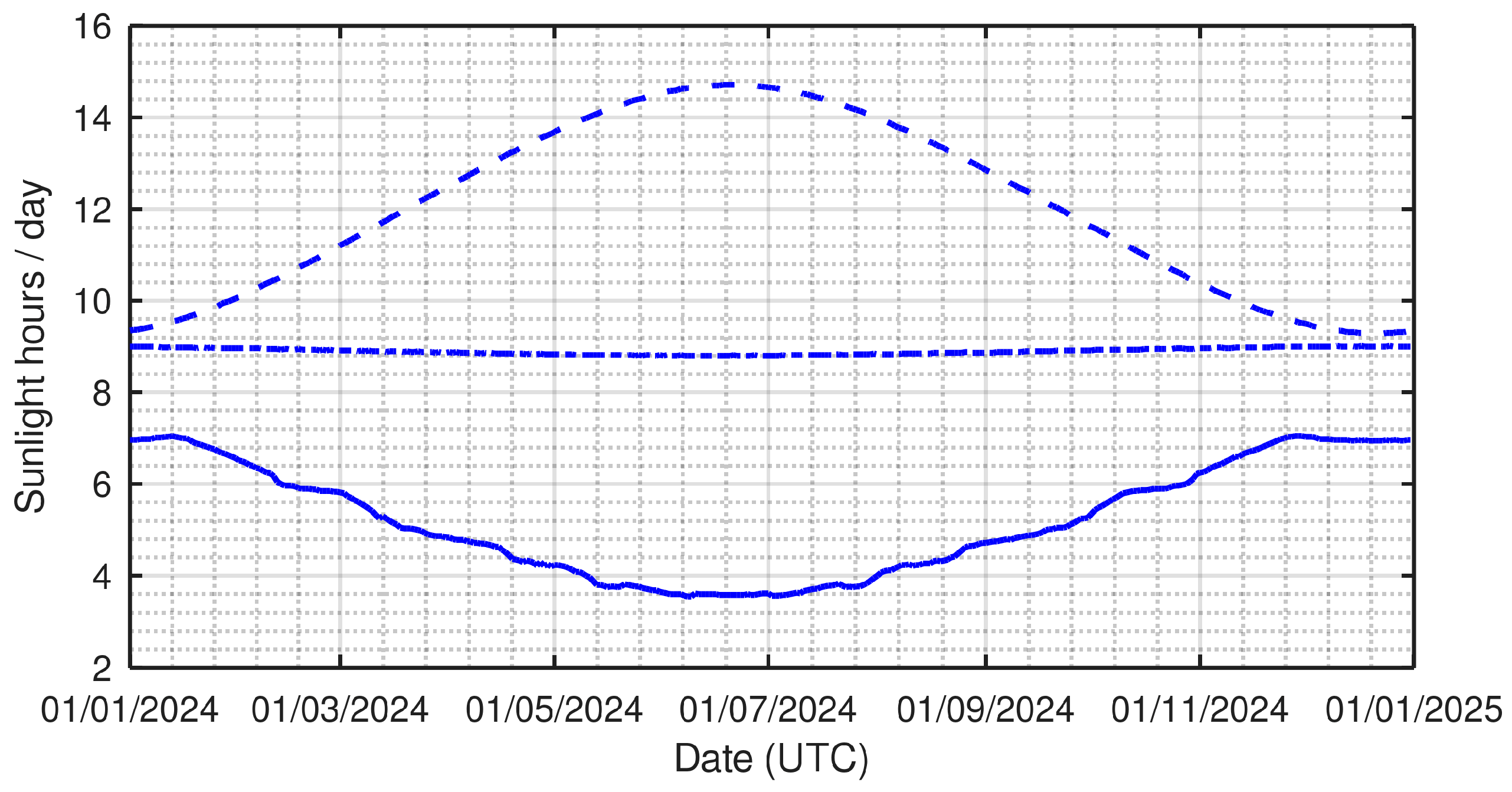
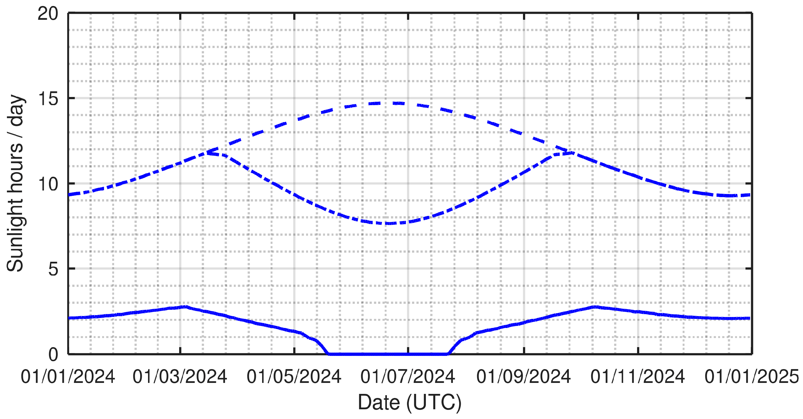
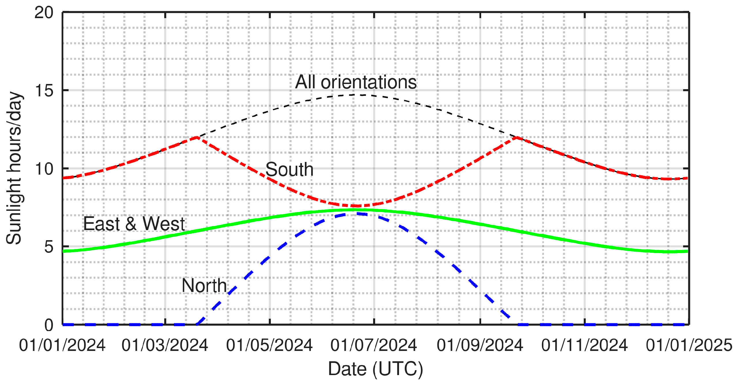
• North (orientation = 0°): No sunlight over the cold half of the year, a small amount of direct sunlight over the warm half of the year, peaking at approximately 7 h at the summer solstice, in two short periods, one at sunrise and the other at sunset (Figure 6).
• East (orientation = 90°): The daily duration of direct sunlight varies from under 5 h at the winter solstice to over 7 h at the summer solstice. The duration profile is the same as the west orientation, but direct sunlight is present in the morning rather than in the afternoon.
• South (orientation = 180°): The orientation with the longest direct sunlight exposure on any day of the year. The peaks occur at the spring and fall equinoxes with about 12 h per day. A local minimum occurs on the winter solstice with just over 9 h and an absolute minimum of under 8 h occurs at the summer solstice.
• West (orientation = 270°): The daily duration of direct sunlight varies from under 5 h at the winter solstice to over 7 h at the summer solstice. The duration profile is the same as the west orientation, but direct sunlight is present in the afternoon rather than in the morning.

It is interesting to note that on the day of the summer solstice, all orientations have approximately the same number of hours of direct sunlight. If the obstacles are considered, the number of sunlight hours will be smaller than the maximum represented in Figure 29.

Case 1 in the results section is a window facing north (orientation = 2.1°), and the view from the window is shown in Figure 5a. The unblocked portion of the view corresponds to the white areas in Figure 5b. This view was mostly unblocked but since the sun reaches the window at very shallow angles it was easily blocked by the window frame and therefore only a small proportion of the available sunlight, which was already very small, reached the inside of the building, as shown by the light gray and white areas in Figure 6. The dash–dotted line in Figure 7 shows the available sunlight hours for a situation with no obstacles and the solid line portrays the actual available sunlight considering obstacles, which shows that for most of the year, no sunlight crossed the window pane and during the summer months there was only about 1 h per day of available sunlight, which was split over two short periods at sunrise and sunset, as shown by the small white areas in Figure 6. Even though the view was not blocked, the availability was only about 4.5% as shown in Figure 8, which indicates that it was very difficult to harness the little amount of sunlight that was available to the northern orientation.

The opposite of Case 1 is Case 4, which faced south (orientation = 177.5°) but was a window with a heavily blocked view as shown in Figure 17a,b. As shown by the light gray and white areas in Figure 18, there was a high potential for sunlight availability, but since the view was heavily blocked, only a small proportion of the available sunlight reached the window. Because the sun’s elevation was high close to midday in the summer (Figure 17b), the sunlight did not cross the window frame, causing a period in the middle of the summer when there was no direct sunlight available, as shown by the zero values at the center of the abscissa in Figure 18, Figure 19 and Figure 20. The average availability for this case was only 16%, as shown in Figure 20, which confirmed that the view was heavily blocked.

Case 2 (orientation = 75.5°, northeast) and Case 3 (orientation = 146.6°, southeast) were similar in the sense that the presence of direct sunlight was shifted toward the morning period. The views in Case 2 (Figure 9a,b) and Case 3 (Figure 13a,b) were mostly unblocked. In Case 2, the potential availability ended at about midday as shown by the light gray area in Figure 10 and for Case 3, it ended at a similar time at the summer solstice and about 3 h later at the winter solstice. The potential total number of hours of sunlight per day for Case 2 varied from approximately four at the winter solstice to seven at the summer solstice (Figure 11), while for Case 3, it was approximately constant at about 9 h per day (Figure 15). Considering the obstacles, the average availability over a year was approximately 60% for both cases (Figure 12 and Figure 16).

In Case 5 (orientation = 255.5°, southwest) and Case 6 (orientation = 326.6°, northwest), the availability of direct sunlight was shifted toward the afternoon. The view in Case 5 (Figure 21a,b) was blocked by vegetation and although the potential availability period went from close to midday until about 5 pm at the winter solstice to about 8 pm at the summer solstice (Figure 22), only a small fraction of direct sunlight overcame the surrounding vegetation. Due to the irregular nature of the obstacles in this case, the duration of the available sunlight was also irregular, as shown in Figure 23 and Figure 24, with an average availability over a year of about 26% (Figure 24). For Case 6, the potential availability with no obstacles ranged from zero at the winter solstice to about 6 h at the summer solstice (Figure 27). The obstacles in this case caused the actual availability to go to zero in the winter period, increasing to about 4 h at the summer solstice, with an average availability after obstacles over a year of about 33% (Figure 28).

The sun tracking represented by the yellow and red dots in Figure 5b, Figure 9b, Figure 13b, Figure 17b, Figure 21b and Figure 25b shows the areas of obstacles in the view field that block sunlight, as well as obstacles that did not play a part in this regard.

Overall, we found that the reduction in available direct sunlight due to the surrounding obstacles was very significant. Therefore, the proposed method has potential for widespread application and can be incorporated into an application on a smartphone.

5. Conclusions

The method we proposed was able to calculate the number of direct sunlight hours for six different test cases and had the advantage of quantifying the obstructions caused by the surrounding obstacles, which we found to cause a significant decrease in the availability of direct sunlight. The time of day when direct sunlight was available to a specific window or other sunlight entry area of a building is shown on a plot, over a year, both with obstacles and without obstacles.

This method has the advantage of simplicity, with a minimum number of input parameters and the possibility to be implemented on a smartphone application.

Future work may include a calculation of the solar energy budget as well as a description of the building materials and geometry, to estimate the temperature evolution and energy consumption over time.

This procedure can be very useful to aid in the decision to acquire real estate, which was our main motivation for this work.

References

1. Hachem, C.; Athienitis, A.; Fazio, P. Parametric investigation of geometric form effects on solar potential of housing units. J. Sol. Energy 2011, 85, 1864–1877. [Google Scholar] [CrossRef]
2. Hachem, C.; Athienitis, A.; Fazio, P. Evaluation of energy supply and demand in solar neighborhood. Energy Build. 2012, 49, 335–347. [Google Scholar] [CrossRef]
3. Hachem, C.; Fazio, P.; Athienitis, A. Solar optimized residential neighborhoods: Evaluation and design methodology. J. Sol. Energy 2013, 95, 42–64. [Google Scholar] [CrossRef]
4. Knowles, R.L. The solar envelope: Its meaning for energy and buildings. Energy Build. 2003, 35, 15–25. [Google Scholar] [CrossRef]
5. Compagnon, R. Solar and daylight availability in the urban fabric. Energy Build. 2004, 36, 321–328. [Google Scholar] [CrossRef]
6. Cheng, V.; Steemers, K.; Montavon, M.; Compagnon, R. Urban form, density and solar potential. In Proceedings of the 23th Conference on PLEA, Geneva, Switzerland, 6–8 September 2006. [Google Scholar]
7. Ghosh, S.; Vale, R. The potential for solar energy use in a New Zealand residential neighborhood: A case study considering the effect on CO2 emissions and the possible benefits of changing roof form. Australas. J. Environ. Manag. 2006, 13, 216–225. [Google Scholar] [CrossRef]
8. Ratti, C.; Baker, N.; Steemers, K. Energy consumption and urban texture. Energy Build. 2005, 37, 762–776. [Google Scholar] [CrossRef]
9. Bellia, L.; Fragliasso, F.; Pedace, A. Evaluation of Daylight Availability for Energy Savings. J. Daylight. 2015, 2, 12–20. [Google Scholar] [CrossRef]
10. Christensen, C.; Horowitz, S. Orienting the neighborhood: A subdivision energy analysis tool. In Proceedings of the ACEEE Summer Study on Energy Efficiency in Buildings, Pacific Grove, CA, USA, 17–22 August 2008. [Google Scholar]
11. Colona, E.C. Potential reduction in energy consumption in consolidated built environments. An analysis based on climate, urban planning and users. VITRUVIO Int. J. Archit. Technol. Sustain. 2018, 3, 47–71. [Google Scholar] [CrossRef]
12. Achsani, R.A.; Paramitasari, A.U.; Sugangga, M.; Wonorahardjo, S.; Triyadi, S. Optimization of daylighting outdoor availability in urban kampung. In IOP Conference Series: Earth and Environmental Science, Proceedings of the 5th HABITechno International Conference, Bandung, Indonesia, 11 November 2021; IOP Publishing: Bristol, UK, 2021. [Google Scholar] [CrossRef]
13. Verso, V.R.M.L.; Antonutto, G.; Torres, S. Sunlight-Daylight Signature: A Novel Concept to Assess Sunlight and Daylight Availability at Urban Scale. J. Daylight. 2023, 10, 136–152. [Google Scholar] [CrossRef]
14. Bellia, L.; Acosta, I.; Campano, M.A.; Fragliasso, F. Impact of daylight saving time on lighting energy consumption and on the biological clock for occupants in office buildings. Sol. Energy 2020, 211, 1347–1364. [Google Scholar] [CrossRef]
15. Tabadkani, A.; Roetzel, A.; Li, H.X.; Tsangrassoulis, A. Daylight in Buildings and Visual Comfort Evaluation: The Advantages and Limitations. J. Daylight. 2021, 8, 181–203. [Google Scholar] [CrossRef]
16. Acosta, I.; Campano, M.A.; Bellia, L.; Fragliasso, F.; Diglio, F.; Bustamante, P. Impact of Daylighting on Visual Comfort and on the Biological Clock for Teleworkers in Residential Buildings. Buildings 2023, 13, 2562. [Google Scholar] [CrossRef]
17. Pol, O.A.; Robinson, D. Impact of urban morphology on building energy needs: A review on knowledge gained from modeling and monitoring activities. In Proceedings of the CISBAT, Lausanne, Switzerland, 14–16 September 2011. [Google Scholar]
18. Leung, K.S.; Steemers, K. Exploring solar responsive morphology for high-density housing in the tropics. In Proceedings of the CISBAT, Lausanne, Switzerland, 2–3 September 2009. [Google Scholar]
19. Kämpf, J.H.; Robinson, D. Optimisation of building form for solar energy utilization using constrained evolutionary algorithms. Energy Build. 2010, 42, 807–814. [Google Scholar] [CrossRef]
20. Morello, E.; Gori, V.; Balocco, C.; Ratti, C. Sustainable urban block design through passive architecture, a tool that uses urban geometry optimization to compute energy savings. In Proceedings of the 26th Conference on Passive and Low Energy Architecture, Quebec City, QC, Canada, 22–24 June 2009. [Google Scholar]
21. Strømann-Andersen, J.; Sattrup, P.A. The urban canyon and building energy use: Urban density versus daylight and passive solar gains. Energy Build. 2011, 43, 2011–2020. [Google Scholar] [CrossRef]
22. Capeluto, I.G. The influence of the urban environment on the availability of daylighting in office buildings in Israel. Build. Environ. 2003, 38, 745–752. [Google Scholar] [CrossRef]
23. Jabareen, Y.R. Sustainable urban forms: Their typologies, models, and concepts. J. Plan. Educ. Res. 2006, 26, 38–52. [Google Scholar] [CrossRef]
24. Ali-Toudert, F. Energy efficiency of urban buildings: Significance of urban geometry, building construction and climate. In Proceedings of the CISBAT, Lausanne, Switzerland, 2–3 September 2009. [Google Scholar]
25. Nault, E.; Moonen, P.; Rey, E.; Andersen, M. Predictive Models for Assessing the Passive Solar and Daylight Potential of Neighborhood Designs: A comparative proof-of-concept study. Build. Environ. 2017, 116, 1–16. [Google Scholar] [CrossRef]
26. Lechner, N. Heating, Cooling and Lighting, 4th ed.; John Wiley & Sons, Inc.: Hoboken, NJ, USA, 2015; pp. 400–450. [Google Scholar]
27. Duluk, S.; Nelson, H.; Kwok, A. Comparison of solar evaluation tools: From learning to practice. In Proceedings of the 42nd Annual National Solar Conference, Baltimore, MD, USA, 16–20 April 2013. [Google Scholar]
28. Alhmoud, L. Why Does the PV Solar Power Plant Operate Ineffectively? Energies 2023, 16, 4074. [Google Scholar] [CrossRef]
29. Shadow Analysis. Tools and Software. Available online: https://www.linkedin.com/pulse/shadow-analysis-tools-software-eduardo-rodriguez-e-i-t- (accessed on 21 September 2024).
30. Computing Planetary Positions—A Tutorial with Worked Examples. Available online: http://stjarnhimlen.se/comp/tutorial.html#5 (accessed on 29 May 2023).
31. Darin Koblick. Vectorized Solar Azimuth and Elevation Estimation, MATLAB Central File Exchange. Available online: https://www.mathworks.com/matlabcentral/fileexchange/23051-vectorized-solar-azimuth-and-elevation-estimation (accessed on 29 May 2023).
Figure 1. Example of a 360° image (rotated 90°).
Solar 04 00026 g001
Figure 2. Camera sitting on a leveled structure attached to a windowsill.
Solar 04 00026 g002
Figure 3. Coordinates transformation from (Az′, El) to (α, β).
Solar 04 00026 g003
Figure 4. Transformation from (α, β) to pixel coordinates (i, j).
Solar 04 00026 g004
Figure 5. Case 1, orientation = −2.1° (north): (a) 360° picture taken from the window; (b) Boolean image where white corresponds to sky and all other regions appear in black.
Solar 04 00026 g005
Figure 6. Case 1, times when the sun was visible. Black: not visible; dark gray: all directions, light gray: −90° ≤ Az′ ≤ 90°, white: considering obstacles.
Solar 04 00026 g006
Figure 7. Case 1, sunlight hours per day. Dashed line: all directions, dash-dotted line: −90° ≤ Az′ ≤ 90°, solid line: considering obstacles.
Solar 04 00026 g007
Figure 8. Case 1, sunlight availability percentage. Solid line: daily ratio of available sunlight with obstacles to without obstacles, dashed line: mean value over of a year.
Solar 04 00026 g008
Figure 9. Case 2, orientation = 75.5° (northeast): (a) 360° picture taken from the window; (b) Boolean image where white corresponds to sky and all other regions appear in black.
Solar 04 00026 g009
Figure 10. Case 2, times when the sun was visible. Black: not visible; dark gray: all directions, light gray: −90° ≤ Az′ ≤ 90°, white: considering obstacles.
Solar 04 00026 g010
Figure 11. Case 2, sunlight hours per day. Dashed line: all directions, dash-dotted line: −90° ≤ Az′ ≤ 90°, solid line: considering obstacles.
Solar 04 00026 g011
Figure 12. Case 2, sunlight availability percentage. Solid line: daily ratio of available sunlight with obstacles to without obstacles, dashed line: mean value over of a year.
Solar 04 00026 g012
Figure 13. Case 3, orientation = 146.6° (southeast): (a) 360° picture taken from the window; (b) Boolean image where white corresponds to sky and all other regions appear in black.
Solar 04 00026 g013
Figure 14. Case 3, times when the sun was visible. Black: not visible; dark gray: all directions, light gray: −90° ≤ Az′ ≤ 90°, white: considering obstacles.
Solar 04 00026 g014
Figure 15. Case 3, sunlight hours per day. Dashed line: all directions, dash-dotted line: −90° ≤ Az′ ≤ 90°, solid line: considering obstacles.
Solar 04 00026 g015
Figure 16. Case 3, sunlight availability percentage. Solid line: daily ratio of available sunlight with obstacles to without obstacles, dashed line: mean value over of a year.
Solar 04 00026 g016
Figure 17. Case 4, orientation = 177.5° (south): (a) 360° picture taken from the window; (b) Boolean image where white corresponds to sky and all other regions appear in black.
Solar 04 00026 g017
Figure 18. Case 4, times when the sun was visible. Black: not visible; dark gray: all directions, light gray: −90° ≤ Az′ ≤ 90°, white: considering obstacles.
Solar 04 00026 g018
Figure 19. Case 4, sunlight hours per day. Dashed line: all directions, dash-dotted line: −90° ≤ Az′ ≤ 90°, solid line: considering obstacles.
Solar 04 00026 g019
Figure 20. Case 4, sunlight availability percentage. Solid line: daily ratio of available sunlight with obstacles to without obstacles, dashed line: mean value over of a year.
Solar 04 00026 g020
Figure 21. Case 5, orientation = 255.5° (southwest): (a) 360° picture taken from the window; (b) Boolean image where white corresponds to sky and all other regions appear in black.
Solar 04 00026 g021
Figure 22. Case 5, times when the sun was visible. Black: not visible; dark gray: all directions, light gray: −90° ≤ Az′ ≤ 90°, white: considering obstacles.
Solar 04 00026 g022
Figure 23. Case 5, sunlight hours per day. Dashed line: all directions, dash-dotted line: −90° ≤ Az′ ≤ 90°, solid line: considering obstacles.
Solar 04 00026 g023
Figure 24. Case 5, sunlight availability percentage. Solid line: daily ratio of available sunlight with obstacles to without obstacles, dashed line: mean value over of a year.
Solar 04 00026 g024
Figure 25. Case 6, orientation = 326.6° (northwest): (a) 360° picture taken from the window; (b) Boolean image where white corresponds to sky and all other regions appear in black.
Solar 04 00026 g025
Figure 26. Case 6, times when the sun was visible. Black: not visible; dark gray: all directions, light gray: −90° ≤ Az′ ≤ 90°, white: considering obstacles.
Solar 04 00026 g026
Figure 27. Case 6, sunlight hours per day. Dashed line: all directions, dash-dotted line: −90° ≤ Az′ ≤ 90°, solid line: considering obstacles.
Solar 04 00026 g027
Figure 28. Case 6, sunlight availability percentage. Solid line: daily ratio of available sunlight with obstacles to without obstacles, dashed line: mean value over of a year.
Solar 04 00026 g028
Figure 29. Direct sunlight hours for different orientations in the region of Lisbon.
Solar 04 00026 g029
Disclaimer/Publisher’s Note: The statements, opinions and data contained in all publications are solely those of the individual author(s) and contributor(s) and not of MDPI and/or the editor(s). MDPI and/or the editor(s) disclaim responsibility for any injury to people or property resulting from any ideas, methods, instructions or products referred to in the content.