Abstract
This paper presents a measurement-based stability analysis of commercially available single-phase inverters in public low-voltage networks. In practice, manufacturers typically do not disclose the parameters of the inverter design, although interactions with the low-voltage network need to be assessed and predicted. State-of-the-art modeling methods require knowledge about the internal parameters. The method proposed in the paper is based on measurements in the laboratory and does not require detailed knowledge about the specific inverter design for the identification of the black-box linear time-periodic representation. The gained information is used for the black-box stability analysis in the frequency range up to 2 kHz, which covers the bandwidth of the control of the inverters. The method is validated for a commercially available photovoltaic inverter in the laboratory. An instability that leads to a shutdown of the inverter is demonstrated, while the critical frequency range is predicted accurately.
1. Introduction
The aim of higher efficiency in the energy sector, especially with respect to electric loads and generators, has led to an increase in power electronic (PE) devices in public electricity networks (e.g., [1]). These PE devices are typically converters (AC/AC power conversion), inverters (DC/AC power conversion), and rectifiers (AC/DC power conversion) and are simply referred to as devices in this article. Interactions between devices and the impedance of the low-voltage (LV) network can cause major challenges with regard to the grid compatibility of those devices [2]. Considering the large number of different device manufacturers with individual design strategies, the interactions of these devices with the public network, characterized by its frequency-dependent impedance, can significantly differ between the makes of devices. In addition, LV networks show a large diversity in terms of their impedance characteristic [3].
A typical study objective is how to ensure a stable operation of the device and how to tune and optimize its parameters. Studies on how to improve the stability, e.g., passive and active damping techniques [4], as well as adaptive control, have become their own field of expertise in power electronics. Many different studies have demonstrated that the devices can become instable and how to analyze these instabilities (e.g., [5,6]). However, most studies were derived from white-box models. In general, such studies can only be performed if the detailed representation of the device under test (DUT) is known, which are usually conducted by respective device manufacturers only. The challenge in field scenarios is, however, that the device manufacturer has no information about the network where the device is going to be installed in the future. Therefore, generic assumptions have to be made with regard to the network impedance characteristic, whose representativeness for typical conditions is not known to the manufacturer.
In turn, the distribution system operators (DSOs) cannot analyze the devices, since the knowledge about their individual parameters is typically not disclosed by the manufacturers. Resulting from the large number of manufacturers, even for the same application, e.g., photovoltaic (PV) inverters, the individual device components can be designed very differently. Nevertheless, the individual device components can be considered and studied for known topologies and parameters by modularizing the generic inverter model [7], but the representativeness of such models for particular makes is not known to the DSO.
On the other hand, the DSOs usually have knowledge about the network impedance at a given point of connection (PoC). For a stable operation of the device and to assess the interactions with the power grid that can affect other grid-connected devices, it is not only important to know that the devices can become instable, but under which conditions a particular device becomes instable. Currently, for compliance tests (e.g., in [8] or the upcoming IEC 61000-3-16), these devices are typically only tested for their harmonic emission under ideal grid conditions, i.e., sinusoidal supply voltage and without supply impedance, but not with regard to their stability. In reality, the devices are subjected to a background voltage distortion and a network impedance that cannot be neglected. Depending on the topology of the specific LV network where the device is installed, the network impedance seen from the PoC of the device can vary largely, e.g., [3,9]. As a consequence, an increased probability exists that an instable operation of the device is triggered.
Stability in a most general definition implies that, under normal operating conditions, the system is able to remain in its equilibrium state and furthermore converge to an equilibrium state if subjected to disturbances (e.g., [10]). For this study, it is inherently implied that the power equilibrium, i.e., balanced active and reactive power at fundamental frequency, is guaranteed. This means that the power provided by generators in the system is sufficient to fulfil the load demand. The stability considered in this paper typically originates from an interaction of the control with the impedance characteristic of the grid-side filter circuit and the LV network at frequencies above the power frequency. The stability analysis is furthermore restricted to a small signal stability analysis in terms of the DC operating point. In order to cover the diversity of network characteristics, probabilistic approaches should be applied [11]. Instabilities are likely to occur within the bandwidth of the control, which is usually at frequencies below 2 kHz. Under these conditions, the stability analysis is called harmonic stability analysis in this study.
The first known harmonic instability occurred in the Swiss railway grid [12], and further occurrences have been reported, e.g., in the Netherlands [13] and Australia [14]. More recently, this phenomenon were also measured in an LV network in Switzerland, where a sudden change in the network impedance characteristic due to the operation of a series voltage regulator was identified as reason for the instability of a PV inverter [15]. Especially for the studies of [13,14,15], the reproduction of the scenario to replicate the instabilities has faced major challenges, since the black-box models of the individual devices were missing and no general method to analyze commercially available devices on the basis of measurements is available.
Therefore, the focus of the proposed method is not to design or optimize a device as in most PE studies, but the stability assessment of commercially available devices without advanced features to avoid instabilities in the harmonic range (e.g., based on online network impedance measurement). This study focusses on single-phase inverters, especially for PV applications that are going to be installed in LV networks on a large scale and that usually have a very simple design without any advanced features. It is implied that the individual inverter parameters are unknown but not changed between laboratory characterization and their grid operation. This requires a method that is applicable without detailed background knowledge so that the device parameters do not have to be revealed by the manufacturer, while still enabling an assessment of the grid compatibility of the devices with regard to individual network characteristics, e.g., by a DSO.
The aim of this paper is to propose and validate a fully measurement-based black-box stability analysis for single-phase commercially available inverters taking the uncertainty of network impedances into account. The study addresses the challenge to evaluate the risk of instabilities for any inverter seen as a black box in relation to realistic network impedance characteristics at the envisaged connection points in the network.
The paper is structured as follows: Section 2 describes the system model and in Section 3, the study approaches are explained according to the state of the art. A general laboratory identification is provided for the inverter in Section 4 while the applied black-box stability theory is described in Section 5. The laboratory validation is presented in Section 6 and Section 7 discusses the impact of the LV network. Lastly, Section 8 concludes the study and refers to future work.
2. General System Model
In this section, the general system model is described briefly to provide the required background knowledge. For this study, the overall system is separated into two parts: the grid-connected, single-phase inverter and the power grid.
2.1. Single-Phase Inverter
In LV networks, low-power applications, e.g., up to 4.6 kW [8], are often connected via single-phase inverters. These inverters can be found in different application systems, such as PV systems or battery storage systems (BSS) when operating in inverting mode. For BSS and PV systems, the overall working principle is similar. The power provided by the DC side can vary for PV systems on the basis of the solar irradiance and for BSS on the basis of the load demand and the implemented control strategy. The time constants of the DC power changes, typically above , generated by the applications are considered significantly larger (>10) compared to the time constants of the inverter control, such that the DC power (operating point) is seen as quasi-stationary and the system can be linearized around this operating point. Therefore, from a black-box perspective, the BSS and the PV are treated similarly.
If the inverters are studied on the basis of measurements, they are analyzed in terms of their frequency-dependent proportionality between the voltage and the current at the PoC. This proportionality is not only restricted to a linear time-invariant (LTI) behavior of the inverter for the relation between voltages and currents at the same frequency. It can also contain a linear time periodic (LTP) behavior in steady state, i.e., frequency couplings between voltage and current components at different frequencies. According to the inverter design, i.e., the topology and the parameters, these frequency couplings, as well as their dynamic response on changes in the grid-side voltage, show significant differences (e.g., [16,17]).
2.2. Power Grid
The power grid, e.g., LV network, can vary largely in its characteristic [3], which is defined by its background distortion and the frequency-dependent network impedance (shortly referred to as network impedance in the further text). For stability analysis, the network impedance is especially of interest. In addition to transformers and the length of cables and overhead lines, all grid-connected equipment has an impact on the network impedance. Connecting more equipment to a network can lead to a shift in the resonance frequency, as well as its level of amplification [18]. In particular, resonances at low frequencies with a high amplification, commonly observed in weak grids, have been found to be a major issue for the harmonic stability of the inverter [15].
3. General Study Approaches
Approaches to study interactions between devices and the power grid can be categorized with regard to the available knowledge into three groups: white-box, gray-box, and black-box approaches.
3.1. White-Box Approach
The most detailed white-box model is the switched model that contains the detailed implementation of all components, e.g., including the semiconductor switches. It can be suitable to neglect or simplify the detailed model for various reasons such as saving simulation time or to ease advanced stability studies. For simplifying the detailed model, different aspects can be considered, such as coupling effects, e.g., coupled (multiple-input, multiple-output—MIMO) and decoupled models (single-input single-output—SISO), the analysis domain, e.g., time domain, dq-domain, sequence domain, and phase domain, and the frequency range of interest, as well as the type of the small signal model, e.g., averaged or linearized models around a chosen operating point [19]. The model of this study is based on a linearized, frequency-coupled model, which is derived as state of the art from the detailed, switched model for formal white-box analysis. This model represents an LTP model and is explained below to understand the generic system characteristics of the inverter for the black-box analysis.
3.1.1. Linear Time Periodic Model
Some model components, such as PI controllers, low-pass filters, and ideal physical components show an LTI behavior, while the discretization of other components, e.g., dq-transform, due to sampling times or the DC link voltage ripple can only be linearized for a steady state operation and result in an LTP behavior of the inverter. This is noticeable, if the inverter is studied as a two-pole device, represented by the terminals at the PoC, as usually required for studies of grid interaction. Neglecting the time periodic behavior of the inverters, e.g., the frequency coupling effect, can lead to major issues regarding the stability analysis of the inverter [20]. The importance of the consideration of the frequency coupling in the stability analysis found in [20] was based on a time-domain white-box simulation.
If the inverter behavior is periodic in time, the simplified LTI representation of the inverter can be extended to a more accurate model in a state space description in terms of
for the real-value system parameter matrices A, B, C, and D with a periodicity of T, e.g., 20 ms or rather one cycle of the power frequency, in the form
And similarly for B(t), C(t), and D(t) with , and as introduced in [21] for the appropriate dimensions of n and m.
3.1.2. Harmonic State Space Model
The Floquet theorem permits that the LTP state space model can be transformed into the frequency domain with constant parameters using the monodromy matrix [22]. Now, Equation (3) can be expanded into the complex Fourier series with
And similarly for B(t), C(t), and D(t). The same applies to the input vector in terms of
with
and respectively for all x(t) and y(t). If substituted into Equations (1) and (2), it is possible to derive the Harmonic state space (HSS) model as
Since the resulting block Toeplitz matrix that results from the Toeplitz transform would contain infinite elements, it is appropriate to reduce the matrices by truncation considering the frequency range of interest with being the order of truncation. With regard to the input and output, it follows
and respectively for and This leads to the harmonic transfer functions (HTFs) with
which are expressed in the form
It can be seen that the system behavior according to Equations (1) and (2) is periodic in time but can be represented as constants for the HSS model. This is of importance to apply linear analysis techniques on the time-varying but periodic behavior. Although the HSS model according to Equation (10) is identified by making use of the detailed knowledge about the device topology and its parameters, the HSS can also be identified by measurements for black-box studies as shown later, such that the white-box approach represents the sophisticated background theory on which the black-box approach also relies.
3.2. Gray-Box Approach
Typically, either the model is entirely known, as in the previous section, or it is entirely unknown, but sometimes the model is partially known. This is considered a gray-box model. If the topology is known but the parameters are unknown, estimation techniques can be applied (e.g., [23]). Another gray-box approach consists of identifying the model components and including this partial knowledge in a generic model. First approaches for the grid-side filter circuit [24] and the DC-link equivalent capacity [25] have been proposed. However, the gray-box approach has not yet received a lot of attraction due to the lack of missing identification methods and the equivalent representation of the device control algorithm.
3.3. Black-Box Approach
The third approach is the black-box approach. This approach is applied if no specific knowledge about the device is available. In this case, it is not possible to calculate the parameters of the black-box model from a white-box model. Consequently, the model has to be identified by measurements. The most common black-box model is the admittance-based Norton model. A further separation can be made into the decoupled Norton model (see Figure 1) that consists of a frequency-dependent current source of the device, i.e., the inverter, with IInv and a frequency-dependent admittance, e.g., YInv, and the more advanced, coupled Norton model, where the latter also includes the frequency couplings between voltage and current by an additional current. This linearized representation usually holds for small signal analyses of low-power single-phase inverters in grid-feeding mode. Grid-feeding inverters require a grid-side voltage uAC at their PoC to operate and will respond to this voltage in terms of a current iAC that is injected into the LV network. The coupled and uncoupled Norton models are typically used for harmonic power flow studies, although these studies are performed in the frequency domain assuming a steady state. However, simulations using these models can run into convergence issues if the boundary conditions of the solver are not fulfilled, such as for instable inverter operations. To the authors’ knowledge, no publications exist about these effects, but they occur regularly and are a current research focus. So far, it has been a challenge to distinguish between inappropriate solver settings and the insolvability of the harmonic power flow equations.
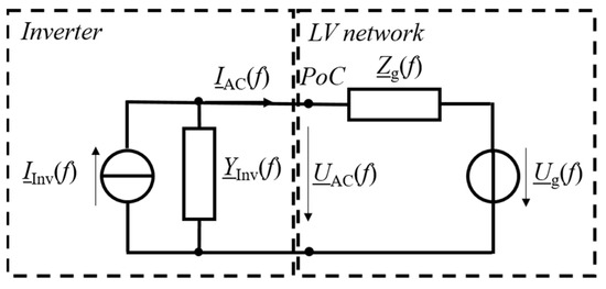
Figure 1.
Admittance-based model of a single-phase inverter (decoupled Norton model) and the power grid.
Currently, black-box time-domain models are not mature enough for dynamic studies, e.g., for simulations of inverter instabilities, although first studies have recently tried to approach this topic by making use of artificial neural networks (ANNs) [26]. Therefore, the black-box approach applied in this study identifies the frequency-domain behavior by measurements and performs a formal analysis afterward.
4. Measurement-Based Identification Method for Black-Box Models
The generic black-box model is shown in Figure 1. It consists of the inverter side and the network side, both represented by a source (voltage or current) and an impedance, or rather an admittance. The subsections below describe the measurement-based methods to identify them. It should be noted that the model is a small signal model, which is intended for an application under the most common quasi-stationary conditions. It is not intended to be applied during short-term events, such as sags, swells, or interruptions.
4.1. Inverter Identification
For the measurement-based identification of inverters, the input admittance of the device is typically identified. For grid-feeding inverters that are typically found in low-power applications in LV networks, a voltage is provided at the PoC, while the current response of the inverter depends on this voltage. Since the admittance will not change, for all stable cases, a specific voltage at the PoC will be periodic and lead to a current response. For all unstable cases, the initial voltage and current, e.g., at the PoC, will increase over time. Nevertheless, the internal inverter parameters, e.g., controller gains and physical filter components, will not change, such that it is possible to identify a general black-box inverter representation independent of the specific input signal characteristics. The interaction between the inverter and a specific LV network can be analyzed, e.g., to predict the stability, by taking the network impedance into account.
To represent the inverter behavior for a specific operating point, a frequency coupling matrix (FCM) Y can be introduced. The voltage and current measurements at the PoC will lead to the discrete elements of the FCM, but not to a continuous description in terms of Y(s). Each FCM element represents the proportionality of a voltage to a current in terms of
while annotates the order of the current harmonic and represents the order of the applied single-frequency voltage harmonic at the PoC. The chosen number of different phase angles of indexed by i allows considering a possible small phase-angle dependency of the frequency coupling element as average. On the basis of initial measurements, the current response of single-phase inverters can be considered approximately linear, i.e., virtually independent from phase angle and magnitude of the PoC voltage.
For LTI systems, a unit step is typically applied to identify the model that causes a broadband excitation. This is not suitable for LTP systems, because of the frequency coupling components that will lead to a superposition in the current spectrum for a broadband excitation. Instead, the constant parameters of the FCM, i.e., the LTP system, can be derived by applying a single-frequency sweep that is superimposed with the supply voltage. A geometrically periodic test signal in the form below,
will be superimposed to the grid-side voltage (t) with the fundamental frequency , i.e., 50 Hz, in terms of
so that the grid-side voltage at the inverter clamps will result in
following [21]. In the literature, this frequency sweep over the order of the voltage harmonic is also called a fingerprint [27], which results in the FCM for the considered operating point. Due to the linearity of inverters, only a single voltage magnitude and phase angle is required as the sweeping component. This study proposes a value of V at 0° in relation to the voltage fundamental according to Equation (13) for . This has been identified as a reasonable amplitude according to measurement experience. Too high distortion amplitudes can cause the inverters to trip, while too low amplitudes of might result in current values with unacceptable measurement uncertainty.
Implementing the frequency sweep to identify the FCM of the inverter, the following steps have to be performed:
- Apply a sinusoidal voltage at the AC side inverter clamps in terms of Equation (14) and measure the multi-frequent current response;
- Superimpose a frequency sweep over for the distortion component defined in Equation (13) by applying Equation (15);
- Measure the multi-frequent current response for each measurement;
- Calculate each element of the FCM according to Equation (12).
Now that the measurement-based representation, i.e., the FCM, has been derived, it can be seen that the FCM and the HSS according to Equation (11) are the same, if the frequency resolution of the HSS is chosen to be the same as the frequency steps in the measurements, e.g., harmonics of 50 Hz and M (order of truncation) being set to 40.
For badly designed inverter systems, the frequency coupling components (also referred to as sidebands) can be dominant and have to be considered in the design process by the manufacturer [20]. Many stability assessment methods, even according to the state of the art, neglect these sidebands (e.g., [28]), because it is analytically challenging to calculate them. For the proposed measurement-based approach, they are included in the measurement results and, therefore, considered as shown in Figure 2 (all components outside the diagonal). If the measured frequency coupling components in the current at order that result from a voltage at order are related to the current at the same order as the voltage, a factor r can be calculated in terms of
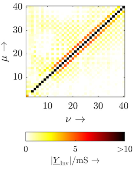
Figure 2.
Frequency coupling matrix of a commercially available PV inverter.
This factor represents the ratio of the impact of the time-periodic to the time-invariant behavior at individual frequencies. Five commercially available single-phase inverters were measured in the laboratory and showed values for r below 10%, thus indicating rather low-amplitude values of the frequency coupling components compared to the respective diagonal component. Consequently, the impact of the frequency coupling components with regard to the network impedance characteristic at other PoCs is low and can typically be neglected. It should be noted that, instead of harmonics, interharmonics can also be used for the model identification. By using specific sets of multiple interharmonics, the identification time can be shortened considerably [29].
4.2. Low Voltage Network Identification
For a reliable evaluation of the risk of harmonic instability for a particular inverter, the range of realistic network impedances that the inverter is expected to be connected to has to be known.
It can be determined on the basis of measurements by injecting a current perturbation into the LV network while observing the resulting voltage response at the PoC. Assuming that the background voltage is constant during the time of measurement, i.e., below 500 ms, the change in the voltage at the PoC can be related to the current change at a given frequency that is forced by the injection of the measurement system so that the network impedance calculates to
While some studies make use of a dedicated measurement system [3], it is also possible to implement the current frequency sweep as a function into the control algorithm (e.g., [30]). This enables an online estimation of the network impedances. However, the latter requires access to the control or at least to the measured data [31,32], although the derived network impedance model is a black-box model and can also be used for the stability assessment.
5. Stability Assessment for Measurement-Based Black-Box Models
5.1. Theoretic Considerations
According to the frequency sweep performed in Section 4, a posteriori, the inverter model including the frequency coupling components is stable for the considered frequency range. As no impedance is connected between inverter and power source, this represents stiff grid conditions. Since it will not be possible to measure the inverter behavior for all grid-conditions, it is necessary to identify the critical conditions theoretically. Furthermore, from a DSO point of view, only the black-box inverter model is available, but not the physical inverter for laboratory tests. Therefore, the stability has to be predicted and cannot be measured.
Often, the formal stability for these cases is performed in the dq-domain for three-phase systems (e.g., [33]). This is not suitable for single-phase low-power applications since the transform into the dq-domain demands the introduction of an artificial three-phase system. For single-phase devices, the individual line-to-neutral characteristic is more representative. In case the inverter can be represented as a controlled current source and an input impedance, e.g., for grid-feeding inverters, the impedance-based stability criterion is suitable for a stability analysis as introduced in [34]. The transfer function of the system has to be known to apply the generalized Nyquist criterion; thus, the system characteristic loci must not encircle the point (−1, 0) for the system to be considered stable. For unknown and complex systems, such as black-box models of inverters, a continuous description of the transfer functions is not always known. From a white-box perspective, the state space model in the time domain can be transferred into the discrete FCM but can also be derived from (black-box) measurements. However, an appropriate reversion back to a continuous description only based on the FCM strictly depends on the interpolation algorithm and has not yet been applied reliably. Therefore, the eigenvalues of the black-box inverter model are not available and cannot be used for the stability analysis.
A simplification by calculating the impedance ratio of the network impedance and the inverter impedance can be evaluated in terms of the impedance-based criterion that has been further developed for interconnected inverter systems [35]. The impedance-based criterion states that, if the network impedance and the inverter impedance intersect, the phase angle of the inverter and the network impedance have to meet
to consider the system as stable. For the state-of-the-art white-box analysis, this is only of limited advantage; thus, eigenvalue analysis can also be used, while, for the black-box analysis, the impedance-based approach solves the issue of not knowing the eigenvalues of the unknown system. Nevertheless, [36] stated that the Nyquist graph test cannot be applied for LTP systems, because of disconnected curves in the image of the imaginary axis in the Nyquist plot. This is why, in [21], the Nyquist criterion was extended to the generalized Nyquist criterion that is applicable for LTP systems. Considering the generalized Nyquist and applying pole zero mapping of the HTF according to [37], the system becomes unstable if the poles of the HTFs with
are in the right half plane (RHP). According to state of the art, the grid-side impedance is represented as an LTI characteristic; consequently, no interaction exists between the frequency coupling elements of the inverter, i.e., all components with |n according to Equation (19) and the LV network. A stable operation regarding the frequency coupling of the inverter is determined in advance by the measurements when identifying the FCM during the frequency sweep. If the impedance characteristic of the LV network also contains frequency coupling components, e.g., if a dominant penetration of devices with strong frequency coupling is present (e.g., six pulse rectifiers), the analysis can be performed by sweeping over n and considering a reasonable order of truncation M that will reflect the bandwidth of the frequency coupling components. Otherwise, the interaction with regard to the network-specific LTI characteristic can be analyzed by LTI analysis. As a summary, Figure 3 shows a scheme of the entire black-box method from the identification to the stability analysis.
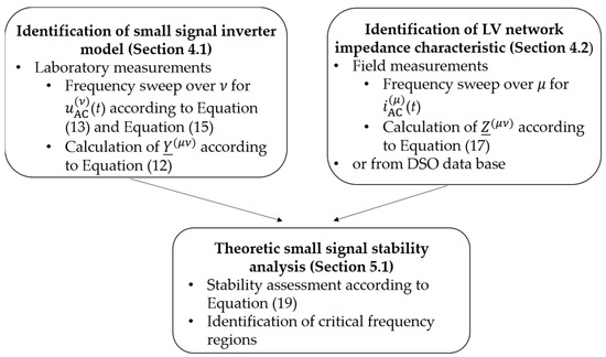
Figure 3.
Overview of the measurement-based black-box stability assessment method.
5.2. Laboratory Validation
Having performed the FCM model identification of a studied, commercially available PV inverter for a given operating point, i.e., a specific DC-level, according to the theory of the impedance-based harmonic stability analysis, an instable condition for the PV inverter is predicted and validated in terms of laboratory measurements.
5.2.1. Test Stand Setup
The test stand consists of the PV inverter, a representation of the network, and a grid simulator that can emulate the background voltage as shown in Figure 4. The PV inverter operates at a DC power level of 1.5 kW (rated power 4.6 kW), and air coils are used to represent the network impedance. The coils have an inductance of about 1.0 mH and 1.3 mH, and both coils and their contact resistances show an overall resistance of 0.7 (sum of R1 and R2 measured at 50 Hz and 1 kHz, Figure 4), which is independent of the frequency up to 2 kHz. Using air coils has the practical advantage that the physical distance of the two coils affects the magnetic coupling in terms of a mutual inductance M. The overall inductance Lg can be calculated following the arrangement of L1 and L2 in Figure 3 according to
and it can be changed by varying the air gap between the coils, i.e., between 2.3 mH (maximum air gap) and 3.2 mH (minimum air gap). Consequently, possible challenging design issues for adaptable coils at power ratings of some kW, which typically require individually manufactured and expensive custom-made products, are avoided. The measurement devices sample at 1 MHz and have an uncertainty lower than 10% for currents higher than and voltages above . The inductance is measured with an uncertainty below 0.5% for inductances above , and the resistance is measured with an uncertainty of 5% for resistances above . Surge protectors (SPD1 and SPD2) are included in the test stand to protect the inverter, as well as the grid simulator, from over-voltages, which can be caused by the air coils.
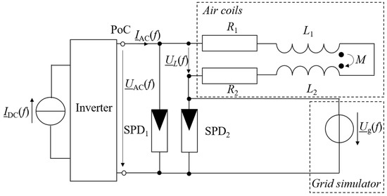
Figure 4.
Equivalent circuit model of the test stand.
5.2.2. Test Cases
To prove the previous theoretic considerations, according to the stability criteria introduced above, different test cases represented by different network impedances are introduced, i.e., test case 1—an almost ideal grid (only parasitic elements of the test stand), test case 2—a weak grid, and test case 3—a critical grid. In all cases, no background distortion is additionally applied, such that the background voltage has a sinusoidal waveform at, (RMS).
As explained previously, the frequency coupling behavior of the inverter is identified as stable and cannot interact with the LV network if the LV network is considered with an LTI characteristic, i.e., according to Equation (19). Therefore, only the diagonal elements of the FCM, i.e., n = 0, have to be considered. The inverter input characteristic and the network impedances of test case 2 (blue) and test case 3 (red) are shown in Figure 5, while test case 1 implies no impact of the network impedance characteristic and is not depicted. It is visible that the inverter shows an injecting behavior (phase angle below 90°) up to about .
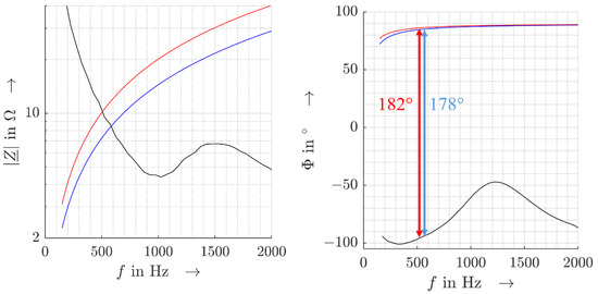
Figure 5.
Impedance magnitude (left) and phase angle characteristic (right) of commercially available PV inverter (black): network impedance of test case 2 (blue) and test case 3 (red).
For test case 1 (ideal grid), the inverter is directly connected to the grid simulator by bypassing the coils. The background voltage is similar to the voltage at the PoC. For test case 2, 2.3 mH is chosen as network impedance (weak grid). Since highly inductive grids, i.e., phase angles close to 90°, represent the most critical conditions, no additional resistance is applied. This resistance would in fact increase the network impedance but at the same time lead to a larger phase margin so that the stability would typically be improved. The minimal phase margin for test case 2 is designed to become 2°. Test case 3 is designed to violate the stability criteria for the inverter. The respective network inductance amounts to 3.2 mH (critical grid). In this case, the maximum phase lag is 182° at 510 Hz, and the inverter is in the instable zone at a loop gain of 0 dB by −2°.
6. Measurement Results
In Figure 6, the results of the voltage at the PoC (a–c), the current injected by the inverter in time domain (d–f), and the injected current in time-frequency domain (wavelet domain) (g–i) are presented for the three test cases. For the wavelet transform , a Morse wavelet with symmetry was applied for the normalizing constant with being the time–bandwidth product in terms of
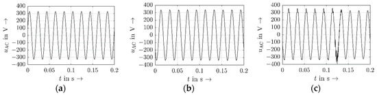
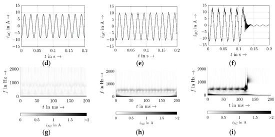
Figure 6.
Measurement results for voltage at PoC for test case 1 (a), test case 2 (b), and test case 3 (c), grid-side inverter current in time domain for test case 1 (d), test case 2 (e), and test case 3 (f), and grid-side inverter current in wavelet domain for test case 1 (g), test case 2 (h), and test case 3 (i).
While the background voltage is purely sinusoidal, the inverter causes voltages at further frequencies at the PoC due to the injected current and its interactions with the network impedance in test cases 2 and 3. Since a stable system is defined as being able to reach steady state after being excited, test case 2 can still be considered as stable, even if the current and voltage show a slight but constant distortion. The system provides enough damping. Increasing the inductance reduces the phase margin and consequently the stability margin. In test case 3, the system cannot provide enough damping anymore, which leads to a much higher distortion component in the current (Figure 6f) and finally causes the inverter to trip. The inverter becomes instable. The respective Nyquist plot is depicted in Figure 7. The anticlockwise encirclement of the point (−1, 0) indicates the unstable characteristic (red curve).
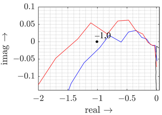
Figure 7.
Nyquist plot for test case 1 (black), test case 2 (blue), and test case 3 (red).
The wavelet representation shows that, as predicted in theory, the frequency range around 500 Hz (see Figure 6) causes the inverter to become instable and eventually to trip. Although the phase margin was only chosen with a phase reserve of 2° (test case 2) and −2° (test case 3) in the instable region, the results match the theoretic considerations very well, demonstrating the high accuracy of the prediction and its applicability with regard to practice. This validates the previously proposed methodology for measurement-based black-box stability assessment if an LTI characteristic of the LV network is assumed.
7. Discussion
Several publications have already shown that inverters can become instable for highly inductive network impedances. However, the inductance values in these studies are unrealistically high with regard to public LV networks (e.g., [34]). Furthermore, existing black-box studies only indicate that the inverters will eventually become instable [38], but provide no experimental proof of the minimal required phase margin in practical applications. In contrast, this study accurately calculates the specific critical conditions for a commercially available PV inverter and validates the preciseness of the fully measurement-based black-box stability assessment. The LV network inductance causing instable behavior identified in this paper, i.e., at 3.2 mH, is still very high, but could occur in the case of very pronounced resonances in the LV network characteristic [39].
The study also provides a proof that the values for the critical frequency range can be estimated with good accuracy. This is of importance, since the impedance characteristic in LV networks varies largely; however, with knowledge about the network impedance, an appropriate prediction of possible inverter instabilities can be made on the basis of the measured FCM of any commercially available inverter. Knowledge about the critical frequency range would also allow design adaptions to prevent an instable inverter behavior at a particular connection point even before its installation. Consequently, in the future, it might be useful if manufacturers publish the frequency-dependent input admittance characteristics as part of the data sheet of their inverters.
This study validates the general application of stability analysis for commercially available single-phase inverters, if the LV network is represented by its LTI behavior. Most public LV networks show a more or less pronounced resonance below 1 kHz [3], which can also be critical to the inverter operation [31]. A larger inductance of the network impedance will shift the resonance to lower frequencies and typically reduce the stability margin even further.
For representing the impedance characteristic of the LV network, the frequency coupling (LTP behavior) is usually neglected so that only the main diagonal (LTI behavior) of the FCM is considered. With an increasing penetration of PE devices along with the decrease of classical generation based on rotating machines, the frequency coupling on the network side will become more dominant and might no longer be negligible. However, so far, no identification method for identifying the LTP network characteristic is available; thus, this is an open research topic.
In addition, first laboratory measurements indicate that not only is the network impedance of relevance for a stable operation of the inverter, but also the background voltage. Although the background voltage will not cause an instability according to the classical definition in control theory, the individual manufacturer design and algorithms for additional services, e.g., anti-islanding (AI) detection, as well as safety precautions such as overcurrent protection, can cause unwanted tripping due to too high distortion levels and critical transients in the voltage at the PoC.
8. Conclusions
A fully black-box-based approach was introduced to predict the stability of commercially available PV inverters without any knowledge about their internal design. The measurement-based approach can be performed in the laboratory and does not require analytic approaches to derive the overall LTP description of the inverter for the analysis.
Future work will address a more detailed analysis of the impact of inverter interactions in LV networks with a high penetration of PE devices. This implies that the LV network itself can contain frequency couplings in its impedance characteristic, which can affect the accuracy of state-of-the-art stability assessment methods. Along with experimental studies, the development of a respective measurement-based identification procedure is, therefore, required. Moreover, the assessment of the individual robustness of an inverter with regard to the combined influence of network impedance, supply voltage distortion, and transients at its connection point will be further developed. The proposed method is dedicated to the small-signal stability of commercially available single-phase inverters under quasi-stationary operating conditions. Events, such as voltage sags, swells, or short interruptions, can also affect the stable operation of a single-phase inverter, but cannot be analyzed by the proposed method and have to be considered in future research. This includes a measurement framework to identify the robustness with regard to events at the point of connection. Furthermore, a holistic framework to test the device performance in terms of the stable operation has to be developed to assess not only the impact of the network impedance, but also the impact of events and the background distortion (subharmonics, interharmonics, and harmonics). In particular, high levels of the background distortion can challenge the stable operation of a device by triggering overcurrent protection or causing the phase-locked loop to trip, which is not covered by the small-signal stability analysis.
Author Contributions
Conceptualization, E.K. and J.M.; methodology, E.K. and J.M.; software, E.K.; validation, E.K. and J.M.; formal analysis, E.K.; investigation, E.K.; resources, J.M. and P.S.; data curation, E.K.; writing—original draft preparation, E.K.; writing—review and editing, E.K., J.M. and P.S.; visualization, E.K.; supervision, J.M.; project administration, J.M.; funding acquisition, P.S. All authors have read and agreed to the published version of the manuscript.
Funding
This work was funded by the Deutsche Forschungsgemeinschaft (DFG, German Research Foundation)—360497354.
Conflicts of Interest
The authors declare no conflict of interest.
Nomenclature
| Symbol | Definition |
| x | Real value |
| Amplitude value | |
| x | Complex value |
| Root-mean-square value/magnitude | |
| Dependency of y on x | |
| |x| | Absolute value |
| x | Column vector |
| X | Matrix |
| Complex matrix element with the indices , |
References
- Blaabjerg, F.; Yang, Y.; Yang, D.; Wang, X. Distributed Power-Generation Systems and Protection. Proc. IEEE 2017, 105, 1311–1331. [Google Scholar] [CrossRef]
- Kocewiak, L.H.; Buchhagen, C.; Sun, Y.; Wang, X.; Lietz, G.; Larsson, M. Overview, Status and Outline of the New CIGRE Working Group C4.49 on Converter Stability in Power Systems. In Proceedings of the 18th International Workshop on Large-Scale Integration of Wind Power into Power Systems as well as Transmission Networks for Offshore Wind Farms, Dublin, Ireland, 16–18 October 2019. [Google Scholar]
- Stiegler, R.; Meyer, J.; Schori, S.; Höckel, M.; Drápela, J.; Hanzlík, T. Survey of network impedance in the frequency range 2–9 kHZ in public low voltage networks in AT/CH/CZ/GE. In Proceedings of the 25th International Conference on Electricity Distribution, Madrid, Spain, 3–6 June 2019. [Google Scholar]
- Ruan, X.; Wang, X.; Pan, D.; Yang, D.; Li, W.; Bao, C. Control Techniques for LCL-Type Grid-Connected Inverters; Springer: Singapore, 2018. [Google Scholar]
- Salis, V.; Costabeber, A.; Cox, S.M.; Zanchetta, P. Stability Assessment of Power-Converter-Based AC systems by LTP Theory: Eigenvalue Analysis and Harmonic Impedance Estimation. IEEE J. Emerg. Sel. Top. Power Electron. 2017, 5, 1513–1525. [Google Scholar] [CrossRef]
- Liu, W.; Lu, Z.; Wang, X.; Xie, X. Frequency-coupled admittance modelling of grid-connected voltage source converters for the stability evaluation of subsynchronous interaction. IET Renew. Power Gener. 2019, 13, 285–295. [Google Scholar] [CrossRef]
- Kaufhold, E.; Meyer, J.; Schegner, P. Modular White-Box Model of single-phase Photovoltaic Systems for Harmonic Studies. In Proceedings of the 2019 IEEE Milan PowerTech, Milan, Italy, 23–27 June 2019; pp. 1–6. [Google Scholar]
- VDE-AR-N 4100: Technical Rules for the Connection and Operation of Customer Installations to the Low Voltage Network (TAR Low Voltage); VDE Verlag: Berlin, Germany, 2019.
- Hernando-Gil, I.; Shi, H.; Li, F.; Djokic, S.; Lehtonen, M. Evaluation of Fault Levels and Power Supply Network Impedances in 230/400 V 50 Hz Generic Distribution Systems. IEEE Trans. Power Deliv. 2017, 32, 768–777. [Google Scholar] [CrossRef]
- Kundur, P. Power System Stability and Control; McGraw-Hill, Inc.: New York, NY, USA, 2004. [Google Scholar]
- Kaufhold, E.; Meyer, J.; Muller, S.; Schegner, P. Probabilistic Stability Analysis for Commercial Low Power Inverters Based on Measured Grid Impedances. In Proceedings of the 2019 9th International Conference on Power and Energy Systems (ICPES), Perth, WA, Australia, 10–12 December 2019; pp. 1–6. [Google Scholar]
- Möllerstedt, E.; Bernhardsson, B. Out of control because of harmonics-an analysis of the harmonic response of an inverter locomotive. IEEE Control. Syst. 2000, 20, 70–81. [Google Scholar]
- Enslin, J.H.R.; Heskes, P.J.M. Harmonic Interaction Between a Large Number of Distributed Power Inverters and the Distribution Network. IEEE Trans. Power Electron. 2004, 19, 1586–1593. [Google Scholar] [CrossRef]
- Moghbel, M.; Glenister, S.; Calais, M.; Shahnia, F.; Carter, C.; Edwards, D.; Stephens, D.; Jones, L.; Trinkl, P. Fluctuations in the Output Power of Photovoltaic Systems Distributed Across a Town with an Isolated Power System Using High-Resolution Data. In Proceedings of the 2019 9th International Conference on Power and Energy Systems (ICPES), Perth, WA, Australia, 10–12 December 2019. [Google Scholar]
- Höckel, M.; Gut, A.; Arnal, M.; Schild, R.; Steinmann, P.; Schori, S. Measurement of voltage instabilities caused by inverters in weak grids. CIRED—Open Access Proc. J. 2017, 2017, 770–774. [Google Scholar] [CrossRef][Green Version]
- Kaufhold, E.; Meyer, J.; Schegner, P. Transient response of single-phase photovoltaic inverters to step changes in supply voltage distortion. In Proceedings of the 2020 19th International Conference on Harmonics and Quality of Power (ICHQP), Dubai, United Arab Emirates, 6–7 July 2020; pp. 1–6. [Google Scholar]
- Kaufhold, E.; Meyer, J.; Schegner, P. Measurement Framework for Analysis of Dynamic Behavior of Single-Phase Power Electronic Devices. Renew. Energy Power Qual. J. 2020, 18, 494–499. [Google Scholar] [CrossRef]
- Busatto, T.; Larsson, A.; Ronnberg, S.K.; Bollen, M.H.J. Including Uncertainties from Customer Connections in Calculating Low-Voltage Harmonic Impedance. IEEE Trans. Power Deliv. 2019, 34, 606–615. [Google Scholar] [CrossRef]
- Rygg, A.; Molinas, M.; Zhang, C.; Cai, X. Coupled and decoupled impedance models compared in power electronics systems. arXiv 2016, arXiv:1610.04988. [Google Scholar]
- Kwon, J.; Wang, X.; Blaabjerg, F.; Bak, C.L. Comparison of LTI and LTP models for stability analysis of grid converters. In Proceedings of the 2016 IEEE 17th Workshop on Control and Modeling for Power Electronics (COMPEL), Trondheim, Norway, 27–30 June 2016; pp. 1–8. [Google Scholar]
- Hall, S.R.; Wereley, N.M. Generalized Nyquist Stability Criterion for Linear Time Periodic Systems. In Proceedings of the 1990 American Control Conference, San Diego, CA, USA, 23–25 May 1990; pp. 1518–1525. [Google Scholar]
- Floquet, G. Sur les équations différentielles linéaires à coefficients périodiques. Ann. Sci. L’école Norm. Supérieure 1883, 12, 47–88. [Google Scholar] [CrossRef]
- Lin, B.H.; Tsai, J.T.; Lian, K.L. A Non-Invasive Method for Estimating Circuit and Control Parameters of Voltage Source Converters. IEEE Trans. Circuits Syst. I Regul. Pap. 2019, 66, 4911–4921. [Google Scholar] [CrossRef]
- Kaufhold, E.; Meyer, J.; Schegner, P. Black-box identification of grid-side filter circuit for improved modelling of single-phase power electronic devices for harmonic studies. Electr. Power Syst. Res. 2021, 199, 107421. [Google Scholar] [CrossRef]
- Kaufhold, E.; Meyer, J.; Schegner, P. Measurement-based identification of DC-link capacitance of single-phase power electronic devices for grey-box modelling. IEEE Trans. Power Electron. 2021, 37, 4545–4552. [Google Scholar] [CrossRef]
- Kaufhold, E.; Grandl, S.; Meyer, J.; Schegner, P. Feasibility of Black-Box Time Domain Modeling of Single-Phase Photovoltaic Inverters Using Artificial Neural Networks. Energies 2021, 14, 2118. [Google Scholar] [CrossRef]
- Cobben, S.; Kling, W.; Myrzik, J. The Making and Purpose of Harmonic Fingerprints. In Proceedings of the 19th International Conference on Electricity Distribution, Vienna, Austria, 21–24 May 2007; pp. 21–24. [Google Scholar]
- Harnefors, L.; Wang, X.; Yepes, A.G.; Blaabjerg, F. Passivity-Based Stability Assessment of Grid-Connected VSCs—An Overview. IEEE J. Emerg. Sel. Top. Power Electron. 2016, 4, 116–125. [Google Scholar] [CrossRef]
- Kaufhold, E.; Meyer, J.; Schegner, P. Fast measurement-based identification of small signal behaviour of commercial single-phase inverters. In Proceedings of the 2021 IEEE 11th International Workshop on Applied Measurements for Power Systems (AMPS), Cagliari, Italy, 29 September–1 October 2021; pp. 1–6. [Google Scholar]
- Riccobono, A.; Liegmann, E.; Monti, A.; Dezza, F.C.; Siegers, J.; Santi, E. Online wideband identification of three-phase AC power grid impedances using an existing grid-tied power electronic inverter. In Proceedings of the 2016 IEEE 17th Workshop on Control and Modeling for Power Electronics (COMPEL), Trondheim, Norway, 27–30 June 2016; pp. 1–8. [Google Scholar]
- Cobreces, S.; Bueno, E.J.; Pizarro, D.; Rodriguez, F.J.; Huerta, F. Grid Impedance Monitoring System for Distributed Power Generation Electronic Interfaces. IEEE Trans. Instrum. Meas. 2009, 58, 3112–3121. [Google Scholar] [CrossRef]
- Mohammed, N.; Kerekes, T.; Ciobotaru, M. An Online Event-Based Grid Impedance Estimation Technique Using Grid-Connected Inverters. IEEE Trans. Power Electron. 2021, 36, 6106–6117. [Google Scholar] [CrossRef]
- Wen, B.; Boroyevich, D.; Burgos, R.; Mattavelli, P.; Shen, Z. Inverse Nyquist Stability Criterion for Grid-Tied Inverters. IEEE Trans. Power Electron. 2017, 32, 1548–1556. [Google Scholar] [CrossRef]
- Sun, J. Impedance-based stability criterion for grid-connected inverters. IEEE Trans. Power Electron. 2011, 26, 3075–3078. [Google Scholar] [CrossRef]
- Liao, Y.; Wang, X. Impedance-Based Stability Analysis for Interconnected Converter Systems with Open-Loop RHP Poles. IEEE Trans. Power Electron. 2020, 35, 4388–4397. [Google Scholar] [CrossRef]
- Desoer, C.A.; Wang, Y.T. On the generalized Nyquist stability criterion. In Proceedings of the 1979 18th IEEE Conference on Decision and Control including the Symposium on Adaptive Processes, Fort Lauderdale, FL, USA, 12–14 December 1979; pp. 580–586. [Google Scholar]
- Wereley, N.M.; Hall, S.R. Frequency response of linear time periodic systems. In Proceedings of the 29th IEEE Conference on Decision and Control, Honolulu, HI, USA, 5–7 December 1990; Volume 6, pp. 3650–3655. [Google Scholar]
- Salis, V.; Costabeber, A.; Cox, S.M.; Tardelli, F.; Zanchetta, P. Experimental Validation of Harmonic Impedance Measurement and LTP Nyquist Criterion for Stability Analysis in Power Converter Networks. IEEE Trans. Power Electron. 2019, 34, 7972–7982. [Google Scholar] [CrossRef]
- Kaufhold, E.; Meyer, J.; Schegner, P. Impact of grid impedance and their resonance on the stability of single-phase PV-inverters in low voltage grids. In Proceedings of the 2020 IEEE 29th International Symposium on Industrial Electronics (ISIE), Delft, The Netherlands, 17–19 June 2020; pp. 880–885. [Google Scholar]


Publisher’s Note: MDPI stays neutral with regard to jurisdictional claims in published maps and institutional affiliations. |
© 2022 by the authors. Licensee MDPI, Basel, Switzerland. This article is an open access article distributed under the terms and conditions of the Creative Commons Attribution (CC BY) license (https://creativecommons.org/licenses/by/4.0/).