Abstract
In the last few years, renewable energies became more socially and economically relevant, and among them, photovoltaic systems stand out. Residential self-consumption of electricity is a field with great potential, and implementation of grid-connected photovoltaic systems (GCPS) is in full rise. The installation of distributed generation systems in residential environments could alter the performance of low-voltage distribution networks, since these are designed for unidirectional power flow and adding these generators means fluctuations in power-flows. For these reasons, a study of the fundamental magnitudes of three low-voltage distribution networks located in Madrid was made for various photovoltaic penetration rates, making use of simulations via the software OpenDSS and subsequent analysis of results. The research concludes that, among other aspects, GCPS produce load flow variations that are dependent on: the penetration rates; the distance from the point of interest and the distribution transformer, increasing the voltage variation between the most productive hours and the night hours with that distance; and on the rate between consumption and generation, so that when it diminishes, the self-sufficiency of the system increases, and with it the voltage of all the buses that tend to the rated voltage. Moreover, there are wide seasonal fluctuations: specifically, in summer months, generation profiles override consumption fluctuations, while in winter months consumption guides voltage and power profiles. Both the code implemented and the results of the analysis were published in an open source website using a free software license.
1. Introduction
In the last few years, renewable energies gained social and economic importance since they are widely available and clean sources. Climate change and issues concerning reliance on fossil fuels are leading to a change of social perspective. They are increasingly seen as an attractive and viable alternative to traditional energy sources. Among them, photovoltaic technology shows some of the greatest potential because it harnesses solar radiation that, to some extent, is constantly beaming onto the earth’s surface continuously. Photovoltaic generation systems implementation is on the rise. However, these systems are dependent on the traditional distribution grid, since generation profiles and household power consumption profiles fluctuate independently based on consumption patterns and weather variables. This results in a need for external energy supplies or accumulation systems to cover all the consumption requirements.
This traditional distribution grid is designed for unidirectional power flow from large electricity generating plants to consumers, with a full-scale central control. There exists a complex interrelationship between all the elements that make up the system. Thus, making substantial modifications is not viable and new technologies should be gradually included. Nevertheless, markets are being driven out to new consumption models, based on auto-consumption, that are more flexible and promote the active participation of customers.
This research analysis systematically explores the effects of a cluster of grid-connected photovoltaic systems (GCPS) on urban distribution networks. Other research analyzed the impact of GCPS in utility networks with large consumption levels, such as town or city utility networks [1,2]. However, our research focuses on the analysis of the network at its lowest level: urban LV distribution networks from the distribution transformer to each building service connection.
The insight provided by this analysis approach has great relevance for two main reasons:
- On one hand, LV distribution networks are grids in which the primary and secondary regulations imposed by the electricity operator (in the case of Spain, Red Eléctrica de España-REE) have no direct influence. These regulations have an impact only upstream the distribution transformer. However, downstream from that point, the relationship between loads and PV-generators can change the operating point of the local distribution network;
- On the other hand, the performance of these LV-distribution networks falls directly on the users.
With the aim of studying these effects, the three fundamental electrical magnitudes are studied: voltage, current, and power flow. In addition, the research deepens into the variables that directly affect these magnitudes, such as energy consumption profiles, energy generation profiles, and incident radiation, among others. As the irregularities of distribution networks caused by the creation of branches according to the needs of urban growth in cities are another major influence on the performance of distribution networks, real distribution networks were studied. Specifically, scenarios selected from a set of blocks with characteristic building typologies due to their construction during periods of major urban growth in the city of Madrid. This fact offers a vision of the problem that leaves behind the study of standard networks to focus on the specific problem of urban distribution networks, with their characteristics and problems, to examine their capacity to face the implementation of grid-connected photovoltaic systems, because it is in the urban environment where their use stands out.
2. State of the Art
Since 2010, the installation of GCP systems with a significant penetration rate were enhanced in some individual locations, and, in consequence, the possibility of real cases studies arose. Prominent among these are the real-case study in Oahu, Hawaii [1], and the one based on the German experience [3], a European country leading the use of renewable energies for auto-consumption. Both highlight the rise of voltage on building service connections above rated voltage, and the rise of flicker noise caused by the generation variability.
However, when modeling and analyzing LV distribution networks with GCPS, assumptions are made because of the limited available data for these networks [4]. These limitations are due either to the amount of variables involved in this process or the absence of real distribution networks with this kind of technology implemented. In this regard, PV system models also exclude several aspects of their behavior and internal characteristics. For example, the performance of a PV system may be affected by a variety of effects such as shadows cast by buildings, trees, or other generators, the hot-spot effect, AC-DC inverter malfunctioning, or electrical faults.
These particular effects are not considered in the analysis either because there is not enough data for a reliable modeling or because they interfere with the understanding of the interaction between a LV distribution network and a set of PV systems. In Section 3.2, detailed information is provided about the assumptions of our analysis.
Most of the studies focus on simulations. Under this approach, the major objective is finding a model based on normalized series that achieve relevant and realistic results, being feasible from the computer workload point of view. Santos–Martín et al. [5] propose a simplified model for analyzing LV networks with a big number of LV-loads connected, reducing the problem to a two-bus equivalent model.
Similar conclusions to those obtained in case studies are drawn by LV distribution network simulations [6,7]. Still on this subject, Ebad et al. [2] and Nguyen et al. [8] study the influence in LV-networks of fluctuations of generation caused by cloud shadows. The models developed by these authors conclude that frequency and voltage variations remain within the technical tolerances if they are randomly distributed along the feeder, which is not always the case when there are centralized generators integrated in the town. Thomson et al. [9,10] explored more deeply the simulation intervals and variables, illustrating the reduction in power losses and transformer load in a specific feeder.
All mentioned research works establish that the implementation of distributed generation systems is generally feasible without substantial changes in conventional distribution networks and they improve the performance of the network in terms of losses and loads. However, additional measures should be taken to monitor and correct deviations caused by high photovoltaic penetration, such as voltage control, energy accumulators, or distribution transformers’ intelligent management [11].
These previous research works are devoted to the analysis of the performance of utility networks or large size distribution generators for feeding large areas in a town or city. Both the individual consumers and small PV systems are aggregated into larger units, and their individual behaviors cannot be separated from one another.
Our research is like a magnifying glass focused on the urban LV distribution networks. It deeply explores the variables that affects the elements (consumers and GCPS) of a cluster in a real distribution network, ranging from the distribution transformer to each building service connection. The analysis is applied to three real locations in the city of Madrid, as explained in Section 3.1.
This analysis was carried out with a software tool developed by the first author.
3. Methods
In this research, to explore the effects produced in urban LV distribution networks caused by GCPS, a software tool was developed based on power-flow analysis. This tool uses EPRI’s OpenDSS as the simulation engine, and Matlab as the data processor and interface. Both the code implemented and the results of the analysis were published in an open source website (https://juliauru.github.io/SGDenBT/, accessed on 13 February 2022) using a free software license. OpenDSS executables and help resources can be found in: https://smartgrid.epri.com/SimulationTool.aspx (accessed on 13 February 2022). More information is provided in the Section 5.
This analysis needs an accurate definition of LV distribution networks with GCPS that defines line performance. With this proposal, four groups of data are used as inputs of simulations:
- Wire characteristics;
- Electrical network topology layout;
- Hourly energy consumption profiles;
- Hourly PV-system generation profiles.
Data acquisition sources and processing methods are detailed in Section 4. Many variables could be calculated in a power flow model but in this case, the output set selected for subsequent analysis is: current module, voltage module, and active power. These magnitudes are calculated in buses selected because of their placement in an outstanding point of the network. All analyzed buses meet one or more of the following conditions set for this analysis:
- Bus placed in transformer terminals (DT);
- Bus placed in load terminals (LT);
- Bus placed in branching points (B).
To ensure delivery of precise results, three real locations in Madrid, which differ from each other in the building typology, were selected. However, the procedure was systematized to extend the investigation to other locations with interesting technical specifications.
For each analyzed scenario, five cases are simulated, varying the photovoltaic penetration rate from 0% to 100%, calculating photovoltaic penetration rate as a percentage of feeders with photovoltaic systems installed. Studied scenarios in Madrid and the reason of their selection are discussed in more detail in Section 3.1.
3.1. Studied Scenarios
In Spain, there is a great potential for photovoltaic systems due to the availability of solar resources throughout its geography, being even greater than those available in other European countries that have a mature photovoltaic market. Studies on this subject obtained, especially in the city of Madrid, global irradiation values of 1.752 on a horizontal surface and of 2.136 on south-facing surfaces with an inclination of 30 [12]. In addition, official data on the energy demand of Spanish households show that more than 90% of domestic consumption could be supplied by solar installations, highlighting the benefit of installing shared-use photovoltaic systems compared to individual ones, as it reduces the variability of consumption profiles and increases the use of energy [12].
The report “Estudio sobre el potencial de generación de energía solar térmica y fotovoltaica en los edificios residenciales españoles en su contexto urbano” [12] determines that, in the case of multifamily dwellings with more than four floors that are the selected scenarios for this research, the implementation of these systems would cover on average 60% of the energy demand due to domestic hot water, 63% of lighting and electrical appliances, and, in the specific case of the city of Madrid, surpluses could be generated that would be between 5–15% in this type of building.
Taking into account the great potential of grid-connected photovoltaic systems in urban environments just explained, three scenarios were selected. All of them are located in Madrid, and each one has a specific building typology that has a major presence in town, since they are the most used during periods of urban expansion.
Furthermore, all of them are zones with multifamily buildings, thus they have three-phase electric connection. They are low-rise buildings, with a predominance of five-storey buildings. This makes the roof surface large enough to produce an amount of energy similar to that consumed by users, thereby favoring auto-consumption. The high rate of homogeneity produces also a lack of shaded areas between buildings, and with it, an homogeneity in generation profiles. Provided that studied areas are not larger than 1 Ha, cloud shadows could be assumed similar in all points of the network. In consequence, the model could be simplified provided all generators receive the same hourly irradiation.
The three chosen scenarios are:
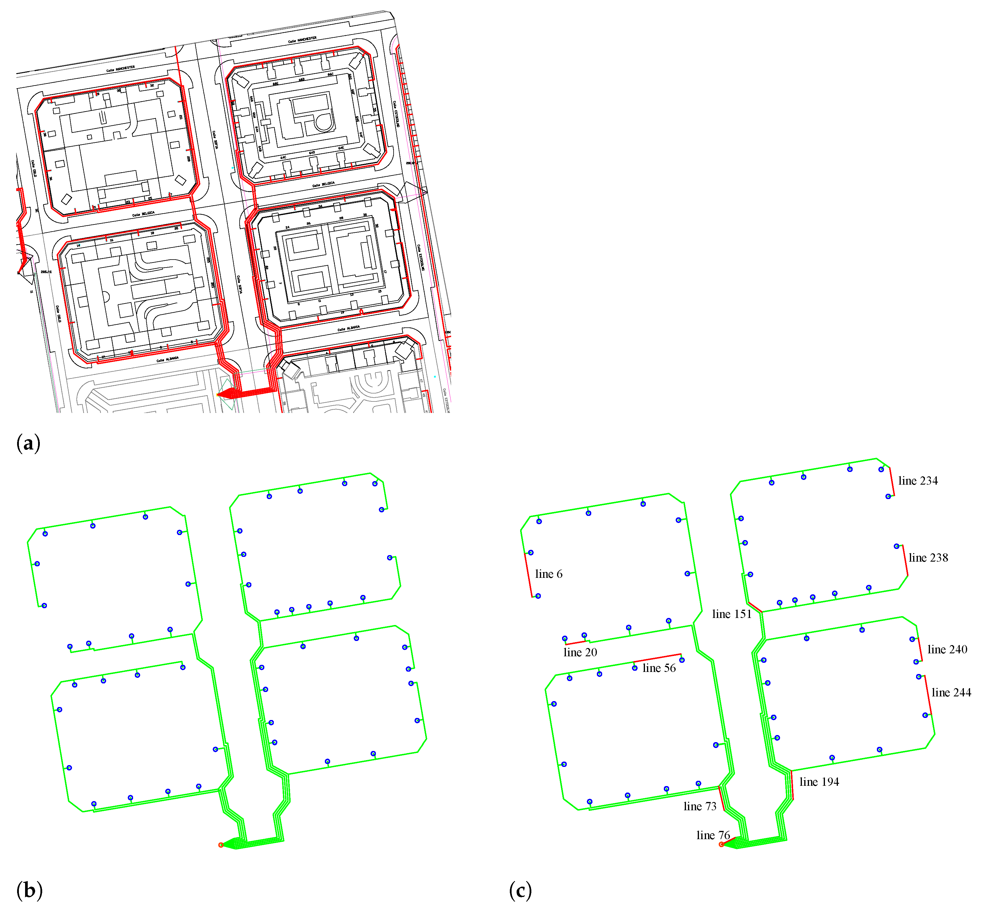
- Scenario 1. Set of buildings fed by a distribution transformer (2 × 630 kVA) consisting of 581 households divided into 48 building service connections. It is composed of five-storey buildings whose topologies are characterized by closed blocks with a large inner patio (See Figure 1a);
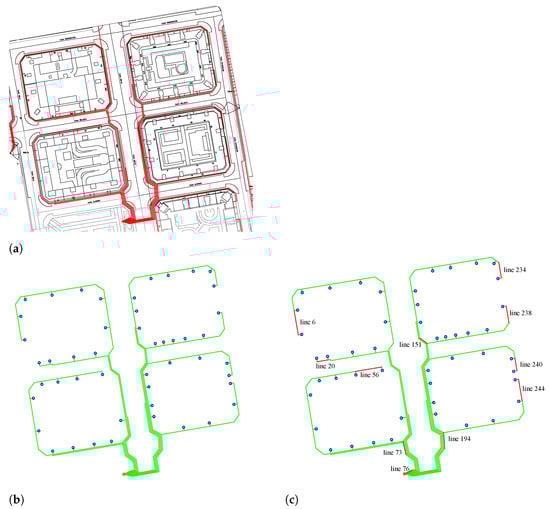 Figure 1. Layout and processed scheme of location Scenario 1. (a) Initial Layout. (b) Simplified geometrical scheme. (c) Scheme with studied lines labeled.
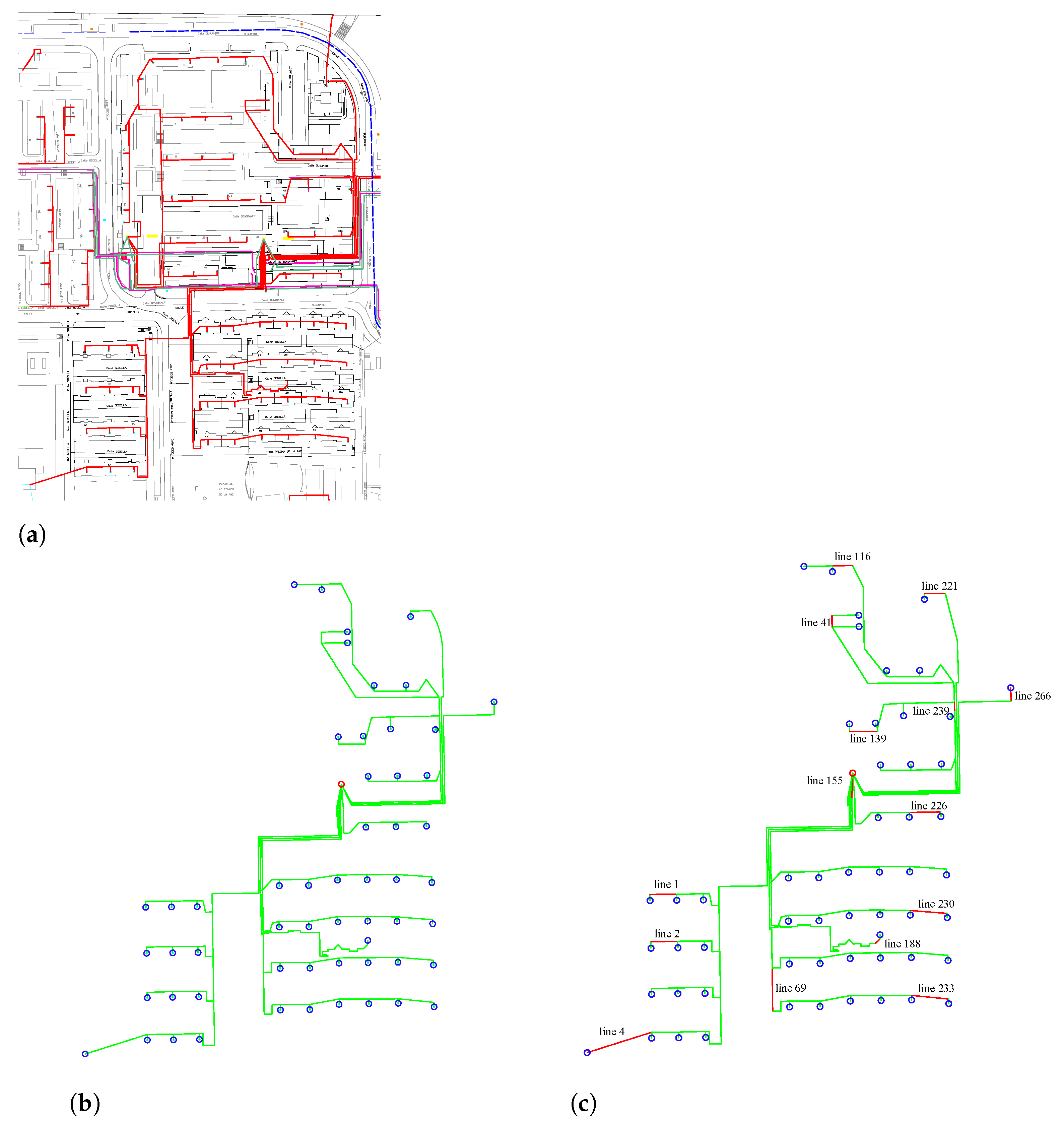
 - Scenario 2. Set of buildings fed by a distribution transformer (2 × 630 kVA) consisting of 560 households divided into 57 building service connections. It is composed of five-storey buildings whose topologies are characterized by linear buildings with two service connections per block (See Figure 2a);
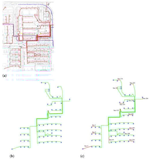 Figure 2. Layout and processed scheme of location Scenario 2. (a) Initial Layout. (b) Simplified geometrical scheme. (c) Scheme with studied lines labeled.
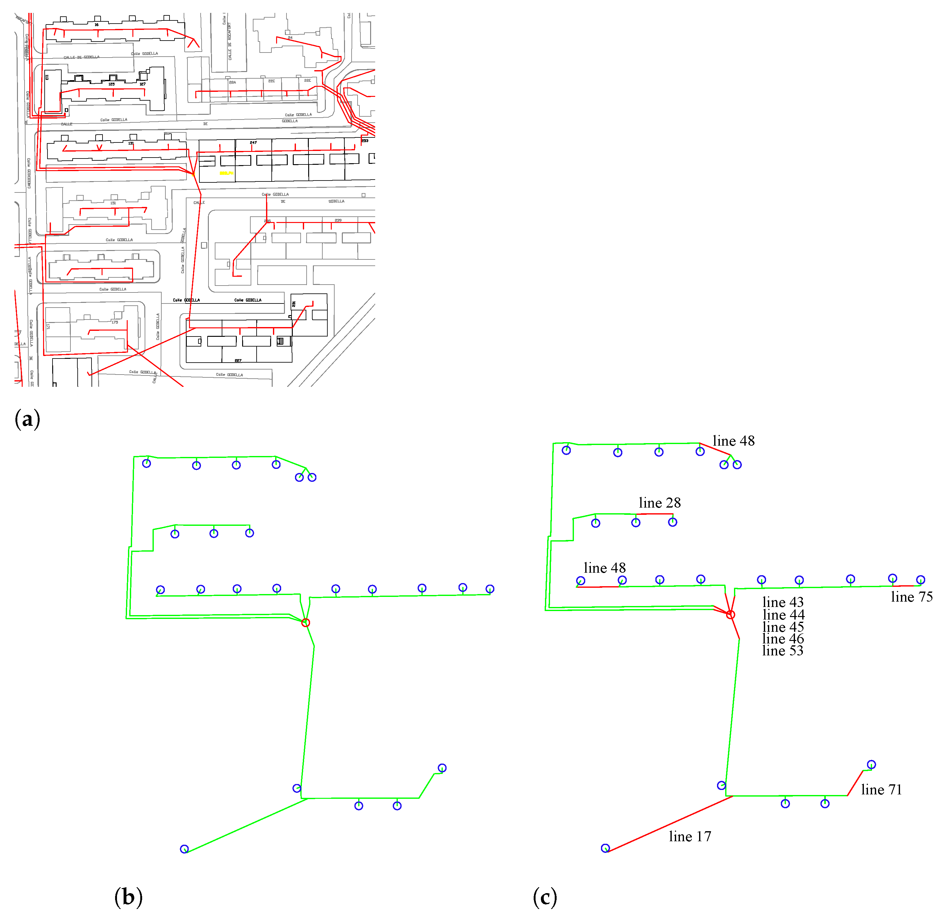
 - Scenario 3. Set of buildings fed by a distribution transformer (630 kVA) consisting of 303 households divided into eight branches. It is composed of five-storey buildings whose topologies are characterized by buildings with H-shape plan view (See Figure 3a).
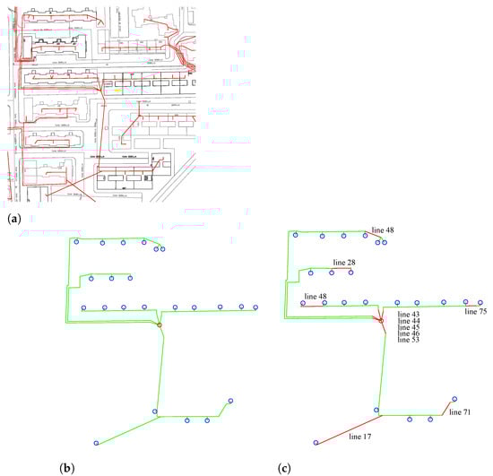 Figure 3. Layout and processed scheme of location Scenario 3. (a) Initial Layout. (b) Simplified geometrical scheme. (c) Scheme with studied lines labeled.
Even if the analysis was carried out for three different scenarios, in Section 6, which presents the research results, examples are mainly focused on the location Scenario 1. Figure 1 shows its layout (complete layout and scheme), and Table A1 collects the lines selected for precise analysis. In Figure 1c, Figure 2c, and Figure 3c, studied lines were labeled with the aim of guiding the analysis developed in Section 6. In this table, field NAME refers to line identification, BUS1 and BUS2 collect the coordinates of buses defining the line (in meters, setting the origin of coordinates at the distribution transformer), and TYPE is the type of line. Even if the analysis refers to elements named lineX, power-flow analysis should be carried out in a specific bus. In consequence, BUS1 of each line is selected.
The analyzed networks have several dozen buses and lines. Therefore, carrying out a detailed comparative analysis of all of them is both unfeasible and inefficient, since the analysis of several consecutive segments of the same line in which there are no representative accidents does not offer a priori additional information on the performance of the system. As the analysis is carried out at specific buses, geometrically representative points were chosen that meet one or more of the following criteria:
- Bus placed in transformer terminals (DT);
- Bus placed in load terminals (LT);
- Bus placed in branching points (B);
- Bus that stands out for its long distance to the DT.
Initially, all the buses meeting any of the four criteria above were listed, and a selection that was representative of the study as a whole was made, taking into account the distribution of the study points and the homogeneity of the network. In addition, emphasis was placed on not eliminating any representative cases, for example, having branches in the study with generators in all iterations and branches that do not meet this criterion; bifurcations and line starts that stand out for having the highest overall load and the lowest overall load, etc.
3.2. Model Assumptions
As previously mentioned, assumptions must be made, and the model has to be simplified when applied to networks with several tens or hundreds of building service connections. For the studied scenarios, the following assumptions were made; however, the research could be extended to fix other variables and analyze the influence of those constant in this experience.
- The system is studied in steady state, using hourly time series of consumption and generation power;
- Generation profiles are the same for all grid-connected systems, since analyzed networks have a reduced extension (less than 10 Ha) and, so, it could be assumed that a similar amount of radiation falls on the buildings roofs at the same moment, and shadows between buildings could be neglected;
- Building service connections are modeled as three-phase balanced loads with a 0.92 power factor;
- Consumption profiles are defined following normalized series, as explained in Section 4.3.
4. Data Source Processing
As exposed in Section 2, power flow simulation based on real distribution networks layouts is a complex problem due to the amount of variables governing the process. Furthermore, this issue is compounded by the lack of real case studies with wide implementation of GCPS. On this basis, simulation definition was obtained based on four fundamental data sources, which were processed and simplified for research requirements accomplishment. Data sources’ acquisition and management are described down below in detail.
4.1. Wire Characteristics
Wire definition is a key element in power-flow analysis for impedance matrix representation. This matrix is calculated according to three main parameters: resistance, dimensions of conductors, and relative position between the conductors that form the lines. This information is not available in open-access platforms since they depend on distribution companies. Due to that, wire characteristics were defined regarding the technical advice of a distribution company. Generally in Madrid, LV distribution lines are designed as shown in Table 1.

Table 1.
Most common wire definitions in Madrid.
4.2. Electrical Network Topology Layout
The analysis departs from general purpose layouts, which include not only electrical line traces, but also general mapping and other supplies information, as shown in Figure 1a, Figure 2a, and Figure 3a. These layouts are simplified eliminating unnecessary elements and geometrically representing only electrical components of feeders. This electric scheme, exhibited in Figure 1b, Figure 2b and Figure 3b, is processed by a Matlab script where the geometrical information is interpreted. Main geometrical elements used to describe electrical components are the type of geometry (point, line...) and the layer where it was drawn. This helps the program to easily adapt to different distribution feeder representations and increase the number of elements involved in the process.
4.3. Hourly Energy Consumption Profiles
Energy consumption profiles depend on many social and economical factors, and for that reason, normalized consumption profiles are used. They are extracted from “Resolución de 16 de diciembre de 2019 de la Dirección General de Política Energética y Minas” [13] of the Spanish Government, since all studied scenarios are located in Madrid. These documents stipulate how electricity distributors should calculate electrical consumption when no measurement was made. They indicate how to approximate that consumption, and normalized profiles are provided. These normalized profiles are the starting point for obtaining hourly energy consumption profiles for this research. The processing of these profiles is set out below to produce variations between loads in the same studied network:
- 1.
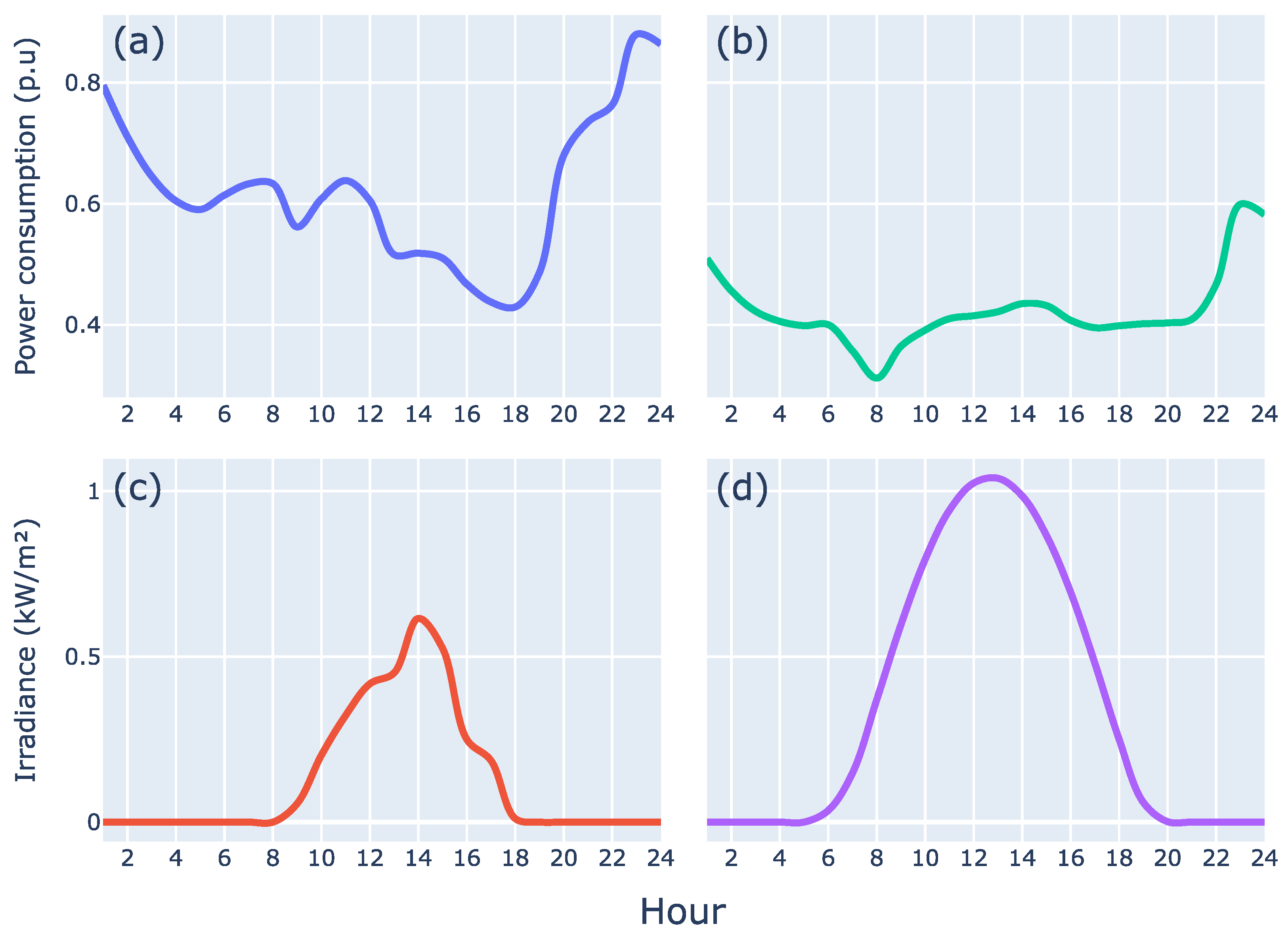
- Profiles are normalized in per unit magnitudes using as base magnitude their maximum value. Figure 4 shows two examples of daily profiles normalized in per unit magnitudes and a comparison with same day irradiation profile;
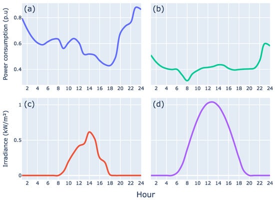 Figure 4. Daily consumption profiles and irradiance profile examples for two specific days: 15 February and 15 June. (a) Daily consumption profile for 15 February; (b) daily consumption profile for 15 June; (c) irradiance profile for 15 February; (d) irradiance profile for 15 June.
 - 2.
- With the aim of obtaining distinct energy consumption profile for each feeder, each point of the curve is randomly varied following a normal distribution with mean the point value and standard deviation of 0.05;
- 3.
- The curve is denormalized with a different power base depending on the building feeder characteristics.
4.4. Hourly PV-Systems Generation Profiles
Since study scenarios are chosen between real groups of houses as explained in Section 3.1, optimal photovoltaic system dimensioning was carried out for the elected buildings with the PVSyst tool. From these simulations made with PVSyst, hourly generated energy profiles were extracted. These hourly generated energy profiles are used to define generators on load terminals with normalized per unit profiles and maximum active power generated.
In this study, the effects of shadows between buildings and other obstacles were not taken into account, since sets of blocks in which the buildings have a similar height (five storeys) were chosen, and therefore, the effect that these would have on the global performance of the system can be neglected. This concept could be introduced in the PVSyst tool, resulting in a specific generation curve for each building. However, including these restrictions for each building would reduce the generality of the study. As previously mentioned, it is assumed that all the curves are similar to each other as they are sets of blocks with a single building typology and in which the calculation and sizing of the PV system were oriented to achieve the maximum generation per building. In addition, these shading effects would mainly influence the early morning and late afternoon hours when radiation is much lower, as can be seen in Figure 4.
5. Software
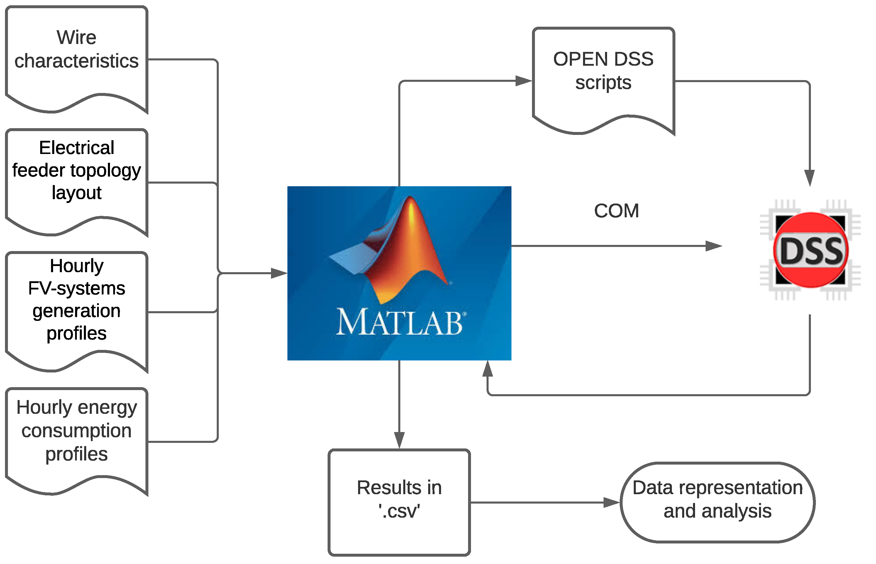
To simulate power flow performance in urban LV networks EPRI’s OpenDSS distribution simulation program is used by implementing a COM connection with Matlab. A software tool was developed in Matlab for including data from different data bases, thus obtaining generality into simulations and dynamically varying parameters. The code is posted on the researcher’s Github repository, https://juliauru.github.io/SGDenBT/ (accessed on 13 February 2022), published under a free software license.
Workflow with this software tool, schematized in Figure 5, was implemented as follows:

Figure 5.
Diagram of simulation workflow.
- (1)
- Data series, exposed before, are saved in text files (in case of consumption and generation profiles) or drawing exchange format files (DXF) (in case of lines definitions), with the format defined in Section 4;
- (2)
- Matlab script is executed. It processes information from files and creates suitable code for OpenDSS platform;
- (3)
- Matlab initializes COM port communication with OpenDSS, and it executes simulation with previously generated code;
- (4)
- Matlab saves all simulations results in CSV files for further data representation and analysis.
6. Analysis of the Results
6.1. Influence of Photovoltaic Penetration Rate
Following the basic concepts of energy transmission, it could be claimed that the lower the consumption, the higher the absolute voltage and the lower power transmitted and current flowing through lines. When the photovoltaic penetration rate in a network increases, the rise of voltage in all the studied points is noticeable, together with the drop of current and active power. This happens because of the reduction in consumption as seen from the medium-voltage side in absolute terms.
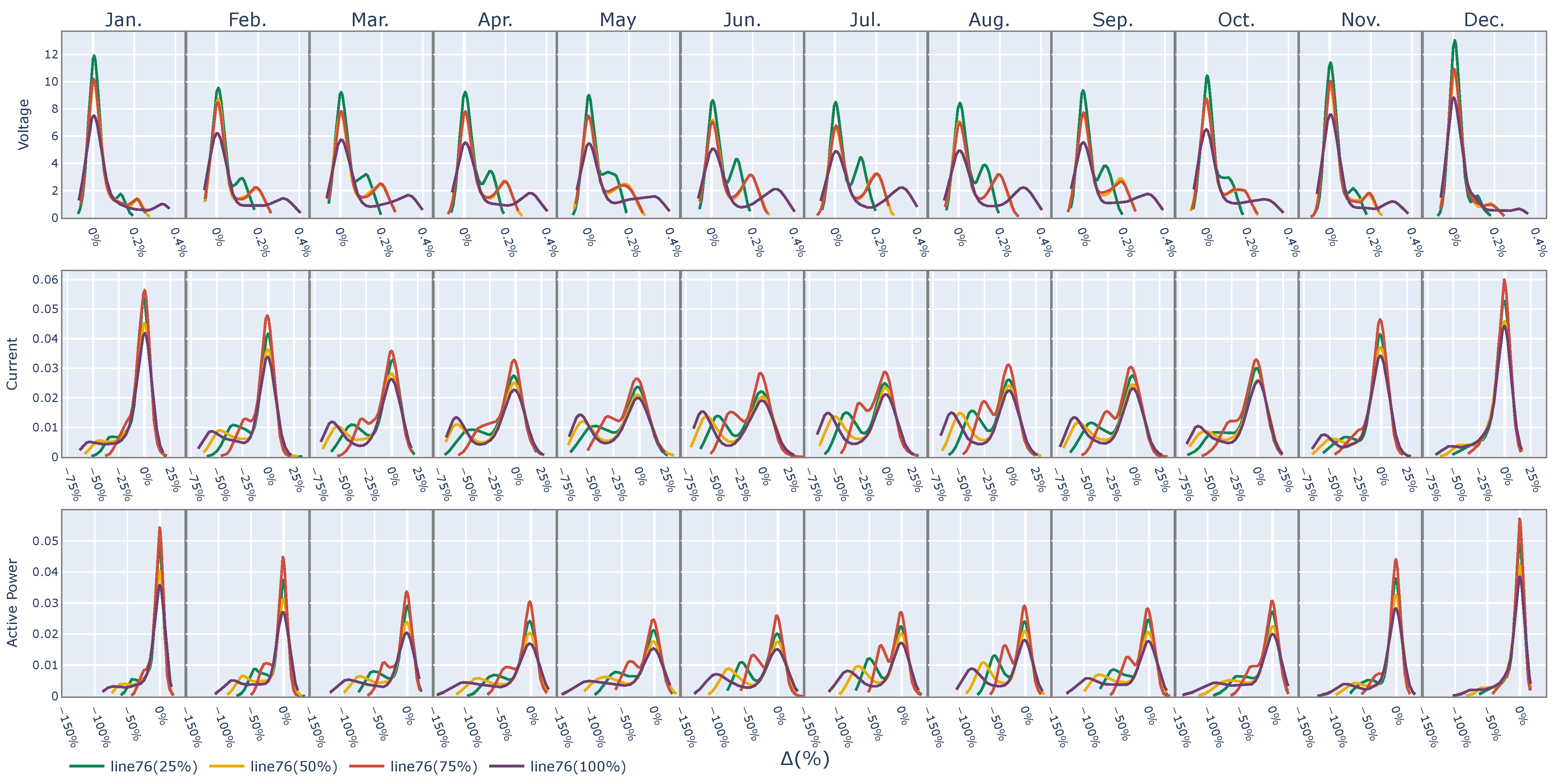
In Figure 6, the distribution probability of voltage and active power percentage variation in a scenario with a certain degree of PV-penetration in comparison with a scenario without generation systems is represented. It means that it is likely that a specific variation occurs, as opposed to the scenario without generation systems. The probability density represents the probability that a certain random variable defined in a given finite range takes a certain infinitesimal value. By its own definition, the area under the curve of this function is unity in the interval between its maximum and minimum value, since it is the sum of the probability of the infinite differentials.
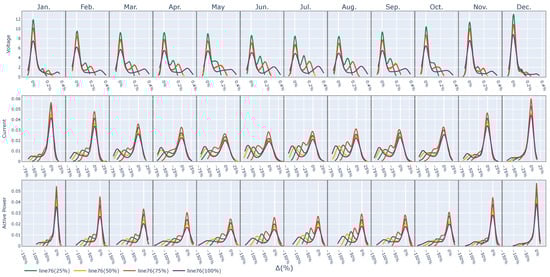
Figure 6.
Distribution probability of voltage, current, and active power percentage variation from a scenario without generation systems. In line76, a bus was placed in transformer terminals for different values of photovoltaic penetration: 25% (green line), 50% (yellow line), 75% (red line), and 100% (purple line).
Therefore, in Figure 6, for the month of January and for the voltage magnitude, the maximum value of the probability density takes a value of 12, while for the same month for the intensity magnitude this maximum value is 0.055. The ranges of the analyzed random variable oscillates between −0.1% and 0.4% in the case of voltage and between −75% and 20% in the case of intensity. If the range of variation of this variable was unitary, the values of the function would obtain values lower than one; however, for the voltage variable (whose maximum is 12), the values taken by the function are much higher because the interval is much smaller (0.5 vs. 1), while for the intensity variable they are lower because the range is much larger (approximately 95 vs. 1).
Figure 6 shows how percentage of 0% variation probability diminishes with penetration rate. Specifically, in July while maximum value for 25% penetration rate scenario is 8.5, for 75% and 100% scenarios it is 6.5 and 5, respectively. It means that when photovoltaic penetration increases, voltage and power values depart from values studied when no PV system is installed. However, a large number of points have a 0% deviation, caused by nightly values that are not hourly affected even if there is diurnal distributed generation.
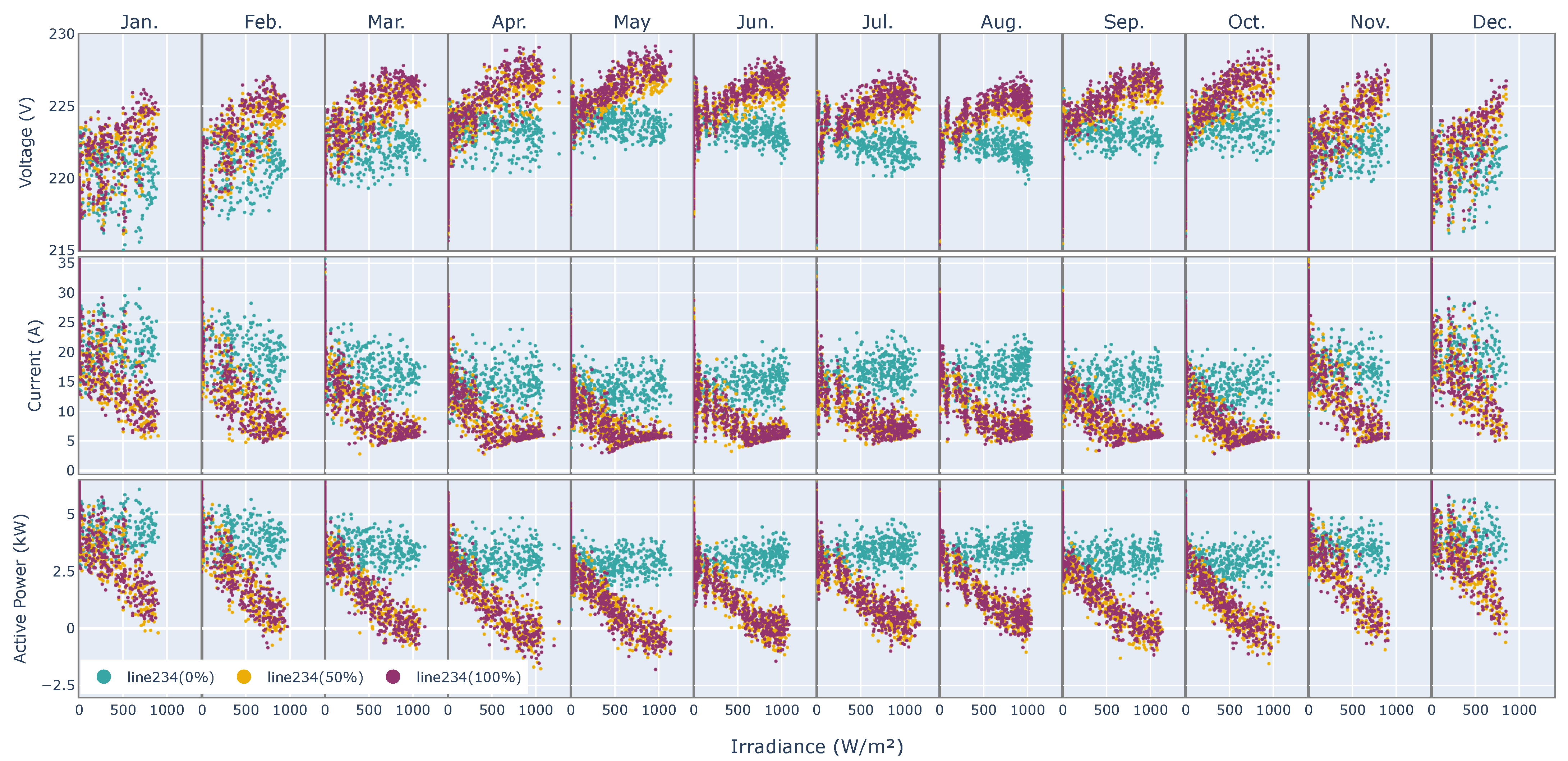
In Figure 6a, bimodality is seen, i.e., while 0% variation peak is decreasing with photovoltaic penetration, a second local maximum appears. This is the most probable value of voltage since, if nightly hours were eliminated, this would be the dominant value, the mean of normal distribution. In summer (July in Figure 6), when generation is higher, bimodality is very marked, while in winter (December) probability distribution is smoothly horizontal. This is due to atmospheric phenomena stability in Spanish summer. Consequently, in summer months generation profiles override consumption fluctuations. In contrast, in winter months consumption guides voltage and power profiles. Figure 7 shows variation of fundamental magnitudes with incident irradiance. This representation clarifies the fact that the hourly voltage distribution is not only caused by an increase in generation in the summer months, but also by the variation of the consumption profile.
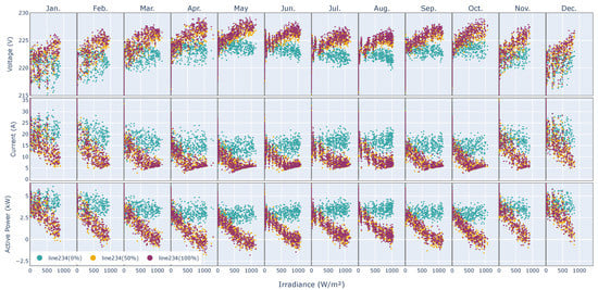
Figure 7.
Scatter plot of voltage, current, and active power evolution with incident irradiance (W/m). In line234, a bus was placed in load terminal for different values of photovoltaic penetration: 0% (blue points), 50% (yellow line), 100% (purple points).
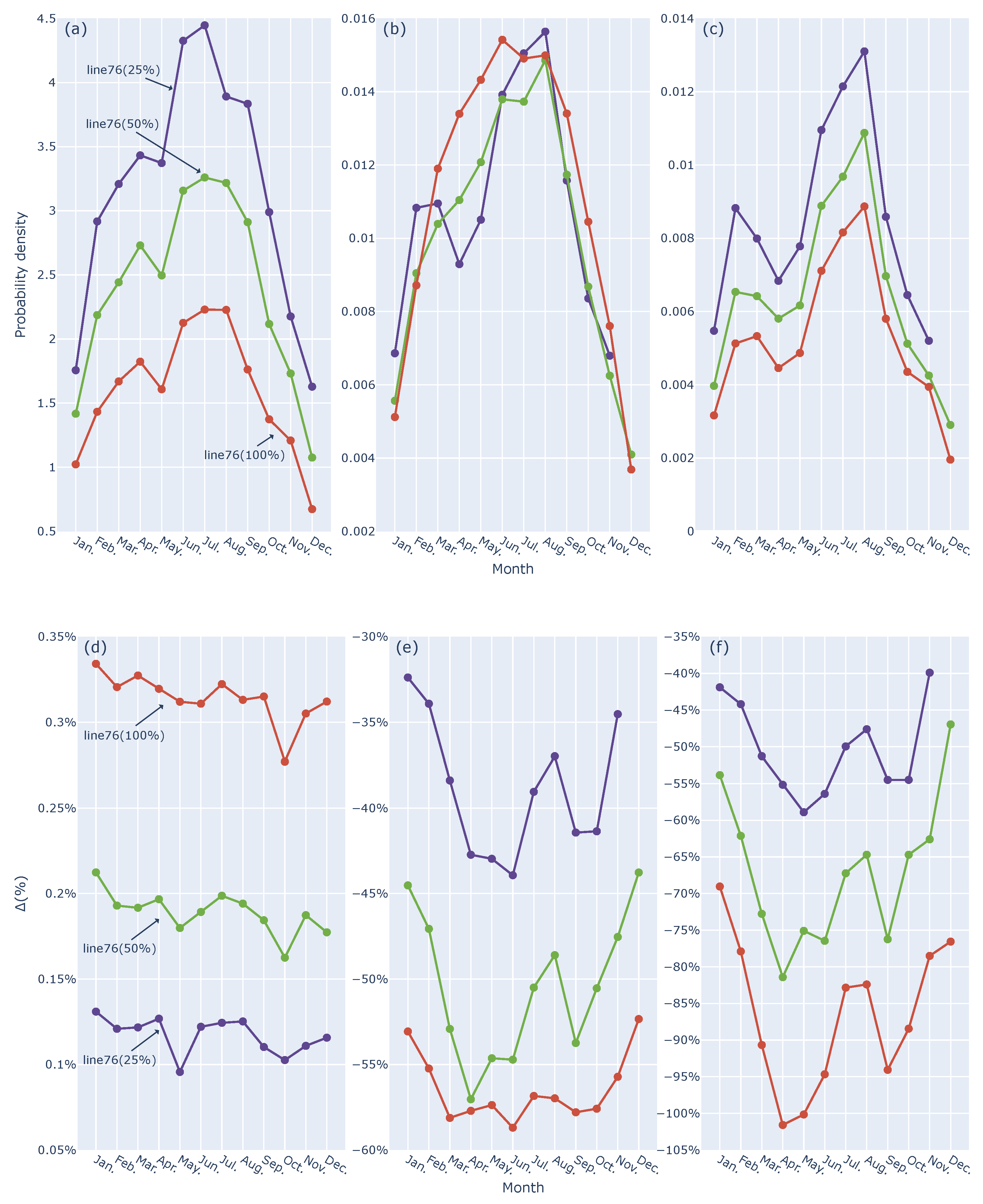
Figure 8 is intended to clarify and summarize the behavior observed in Figure 6. In each of the subplots of this figure, the monthly evolution of two parameters is displayed. On the upper row, the second local maximum value of the probability density function is shown, because the maximum value is centered on the variation with value 0%, which corresponds mostly to the night hours, as mentioned above. On the lower row, the displacement of this second modal maximum along the x-axis is represented, i.e., which variation of the fundamental magnitude will be more probable on a monthly basis.
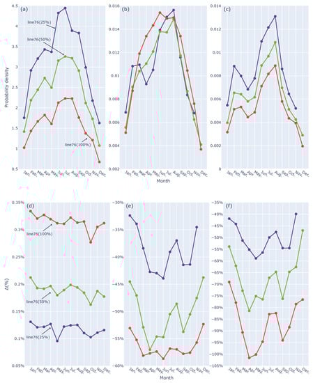
Figure 8.
Monthly evolution of most probable value of voltage, current, and active power, neglecting maximum with 0% variation. Upper row displays density probability of most probable variation: voltage (a), current (b), and active power (c). Lower row displays most probable value of percentage variation of fundamental magnitude with respect to case with 0% photovoltaic penetration rate: voltage (d), current (e), and active power (f).
Figure 8 shows that, for the bus voltage located at line76, the probability increases in the central months when there is greater climatic stability in Spain. However, the monthly evolution of the most probable value (Figure 8d) does not undergo significant variations. On the other hand, the evolution with the photovoltaic penetration is clear, having an annual average value of 0.325% for the case with 100% photovoltaic penetration, while this displacement has an average value of 0.125% per year in the case of 25% photovoltaic penetration.
The Figure 8b does not reveal a clear difference in the value of the probability density of the current maximum with PV penetration, as seen with voltage. In addition, the trends are less uniform as they depend on both generation and system demand profiles. Both current and power evolution do show a trend in the most probable variation of current and power. This effect follows a trend inversely proportional to the variation in the probability density. That is, the maximum is further away from the value without percentage variation of current and power compared to the case without PV penetration, and is more likely in the central months than in the winter months. Therefore, current and power take values in a greater range in these months as a result of demand and generation profiles.
6.2. Influence of the Distance between the Studied Bus and the Distribution Transformer
As explained in Section 6.1, voltage rises with penetration rate while active power and current decrease. However, this variation also depends on the studied bus position within the distribution network. Research shows that the presence of photovoltaic distribution generators increases the voltage in buses placed at load terminals at a higher rate than in the start of lines. This is due to not only the effect of distributed generators, but also the reduction in power losses produced in lines which in an scenario without photovoltaic systems causes a voltage in lines lower than the nominal one. Power and current variate in the opposite sense, since the higher variation is produced in lines placed in distribution transformer terminals, where power is not covered by auto-consumption system flows. As a result, if there exist generators all along the network, current decreases proportionally with the number of generators.
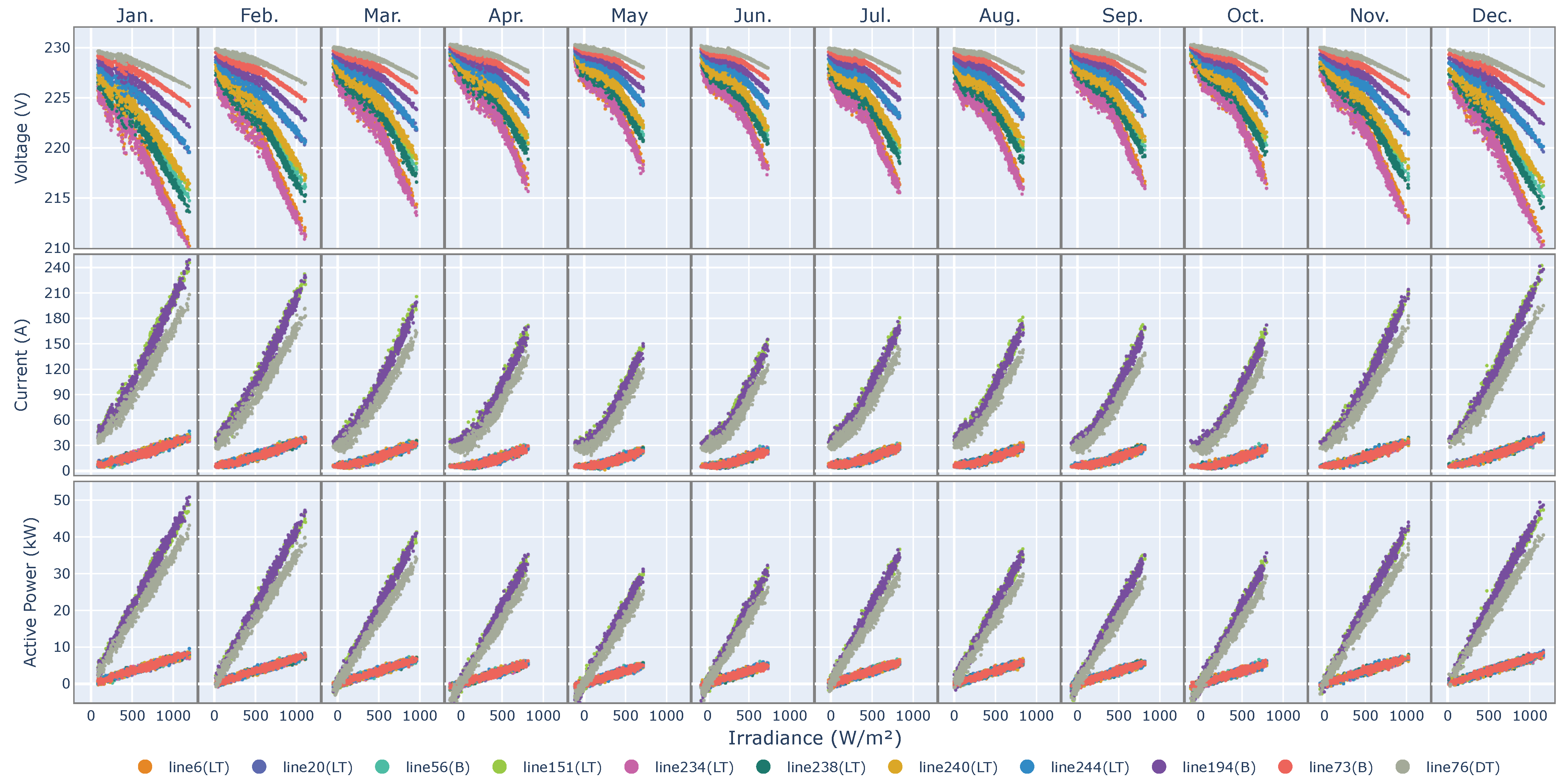
Following this idea, a bus for each one of the three characteristic positions in network is selected to illustrate the difference between them: line234, placed at load terminals; line151, placed in a bifurcation point; and line76, placed in distribution transformer terminals. Figure 9, where voltage and active power of these selected buses in function of incident irradiance is plotted, shows that the fluctuation between voltage in most productive hours and nightly hours increases as the point is getting further from the distribution transformer. This variation calculated for line234, line151, and line76 is respectively, 2.6%, 0.87%, and 0.43%. This variation is directly proportional with the penetration rate and incident irradiance.
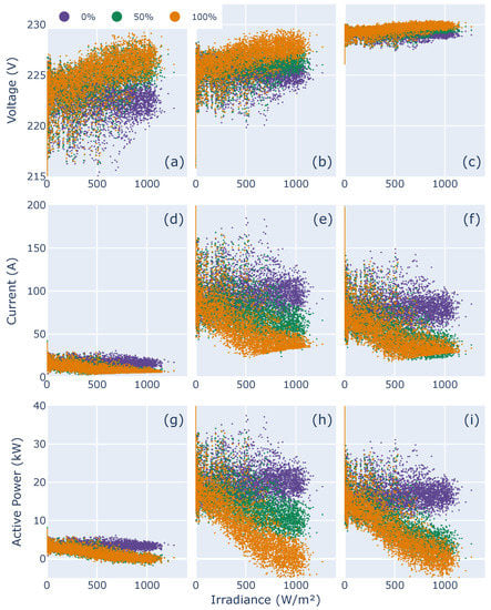
Figure 9.
Scatter plot of hourly data of voltage module (V), current module (A), and active power (kW) versus incident irradiance (W/m) for a complete year. Comparative between three studied lines: line234, bus placed in load terminal (subfigures (a,d,g)); line151, bus placed in a branching point (subfigures (b,e,h)); and line76, bus placed in transformer terminals (subfigures (c,f,i)), for different values of photovoltaic penetration: 0% (blue points), 50% (green points), 100% (orange points).
However, power and current do not follow a direct proportional variation with penetration rate, but they follow a pattern dependent on generators placed downstream the studied bus. In Figure 9, while in voltage subplots variations in three studied buses follow the same trend, it is not the case in active power subplots where three different trends are shown. In line234 there are two marked patterns that correspond to the case where there is a photovoltaic system in load terminals or not, and in line151, there are three distinguishable patterns driven by the number of generators downstream of the studied bus. This demonstrates the influence of generators near the studied bus and those downstream of it over other generators placed further.
6.3. Influence of the Ratio between Generated and Consumed Power
Another major variable of influence is the amount of energy that the conventional grid transfers to the studied feeder. This amount of energy is hourly estimated as:
where
- : energy that conventional grid transfers to the studied feed per hour
- c: number of costumers (loads) of a network
- g: number of generators related with a penetration rate
- : average consumed energy by load and hour
- : average generated energy by photovoltaic system and hour
- i: index of hour
The way the fundamental magnitudes are affected by this amount of energy is shown in Figure 10 for all the studied lines and a scenario with 100% penetration rate (all the buildings have installed a PV system). On this basis, the first remarkable aspect is that, in summer months, there are a small number of hours when the energy that the conventional grid transfers to the studied feeder takes negative values. These hours are the ones when the whole studied feeders are completely self-sufficient (self-sufficiency describes the amount of photovoltaic energy generated in relation to the total amount of energy consumed by the system.), and this means that all the consumed energy is generated inside the network and some kilowatts are discharged into the conventional grid.
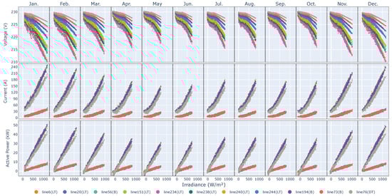
Figure 10.
Scatter plot of voltage, current, and active power evolution with total power provided by conventional electric grid. Comparative of 11 studied buses of Scenario 1 with 100% penetration rate.
In addition, while self-consumption rate rises (moves to the left in the X-axis), voltage in all points of the network rises following mainly two trends. When there is a low self-sufficiency rate, the voltage decreases linearly with externally provided power; however, it loses this linearity when self-sufficiency rate increases, approaching 230 . Consequently, when self-sufficiency rate increases, voltages become more similar between them, independent of their location, and approaching its value to the rated voltage. For example, if only values calculated in the 100% penetration rate scenario are compared (Figure 10), highest variation between points in distribution transformer terminals and load terminals in February is 6.5%, while in May (higher self-sufficiency rate) it is only 1.3%. Active power varies linearly with the amount of energy that conventional grid transfers to the studied feeder because of definition of that magnitude. However, active power scatter plot in Figure 10 shows the zero-crossing point below which the system as a whole is fully self-sufficient.
The reduction in voltage between lines benefits the power losses decrease and the load efficiency, provided that voltages do not grow beyond safety and legal limits.
6.4. Influence of Building Typology and Network Topology
Once the general aspects were analyzed, in this section some aspects about how the building typology and network topology affects the performance of LV distribution networks are briefly stated as a result of comparing the analysis of three scenarios.
On the subject of building typology, systematic analysis was not developed since influence of consumption patterns and proper details of photovoltaic systems implementation should be taken into account; thus, analysis should be extrapolated to hundred of locations with different social and technical features. However, as explained in Section 6.3, if self-sufficiency rate grows in the whole network, voltage rises approaching the load terminals voltage to the distribution transformer terminals’ voltage.
On the subject of network topology, voltage and power fluctuations are exacerbated by network extension and its irregularity.
When comparing two scenarios with different amount of branching points, they differ in the voltage increment between load terminals. While the voltage increment in the most regularly studied scenario could be approximated to zero, in the other one it rises to 0.5%. It is caused by branch irregularities, such as load imbalances or differences between line lengths.
Regularity also affects number of loads per branch that weigh mostly on power and current performance rates. Other irregularity factors could be taken into account in further research such as single-phase loads, different consumption trends, or electric characteristics.
To avoid load imbalances, in networks with large irregularities and a high photovoltaic penetration degree the location of PV generators should be carefully analyzed.
6.5. Seasonality and Hourly Profiles
Since photovoltaic generation changes with irradiance as well as consumption profiles are related to meteorological factors and fluctuations in voltage, current and active power are subsequently intensified in certain daytime hours and seasons.
The larger voltage fluctuations are produced at the central hours of the day when the effect of off-peak demand hours is added to the increment of photovoltaic generation. Magnitudes at days with low peak-irradiance are mainly driven by consumption profiles. Comparison between winter and summer months in Figure 10 reflects how in the colder ones the cloud of points has a larger data dispersion, and they are mainly driven by consumption profiles (as shown also in Figure 6 and Figure 7, which show December’s lack of variation with photovoltaic penetration), while in summer, this dispersion is reduced. This is caused by Spanish summer daytime weather, which means more climatically uniform days and less common cloudiness. In addition, power and intensity are more sensitive to irradiance fluctuations than voltage that grows gradually.
7. Conclusions
A software tool for analysis of urban LV-distribution networks based on data from different sources was developed to study the effects on lines of large penetration rates. This tool uses OpenDSS as simulation engine and Matlab as data processor and interface. It offers flexibility in source data and studied scenarios election. Specifically, in this research three selected scenarios located in Madrid were studied, deepening insights into the variables that directly affect the three fundamental magnitudes. Both the code implemented and the results of the analysis were published in an open source website, https://juliauru.github.io/SGDenBT/ (accessed on 13 February 2022), using a free software license.
This study, which leaves behind the study of utility networks and large size distribution generators for feeding large areas in a town or city carried out in other research, analyzes a cluster of real LV-distribution networks in Madrid from the distribution transformer to each building service connection. This perspective is of great importance because the performance of this grid directly affects users, and the traditional primary and secondary power controls imposed by the electricity operator do not have a direct downstream influence on the distribution transformer.
Results demonstrate that the voltage in buses rises with PV penetration rate, while active power and current decreases. However, at least in our analysis, this trend is also defined by weather variables, most likely because Spain has a remarkable atmospheric phenomena stability. Due to that, in summer months, generation profiles override consumption fluctuations. In contrast, in winter months consumption guides voltage and power profiles.
In addition, these variations of fundamental magnitudes depend on the studied bus position within the distribution network. Specifically, variation between voltage in most productive hours and nightly hours increases as the point gets further from the distribution transformer. This variation is directly proportional to the penetration rate and irradiance incident on the generator. However, power and current do not follow this linear trend, but a pattern dependent on generators placed downstream to the studied bus does instead.
If the urban distribution network is analyzed as a whole, when the self-sufficiency of the global system increases, voltages may raise in all studied buses whose values approach the rated voltage. Consequently, voltage differences between all the buses of the network decrease and losses are reduced too, resulting in a better load performance (if rated voltage is not surpassed). Other factors affecting the network performance are network topology and building typology.
Finally, two related research lines are of interest:
- Energy forecasting.Forecasting the AC power delivered to the grid by a PV system is a research area of considerable importance [14,15]. Both plant owners and electric system operators can benefit from forecasting because it helps to minimize technical risks to the grid, reduce expenses related to the uncertainty of generation, program the dispatch of conventional power generators, and maximize profits with the sale of electricity. Although the usefulness of forecasting is clear in the context of utility-scale PV plants, its application with small-scale urban systems is not direct. Individual owners of the systems are not interested in this approach, and the network operator cannot make decisions based on the future performance of the individual systems. However, forecasting the long-term aggregated performance of a group of systems in a definite urban area could provide useful information for taking decisions on network modifications or improvements, or for the inclusion of new agents such as a fleet of electrical vehicles. The methods and tools developed in this paper can be combined with a PV power forecast procedure, such as the one developed in [16], which is left as a future line of research.
- Grid expansion and optimization.As previously stated, the integration of photovoltaic systems in urban low-voltage grids is generally feasible without substantial changes in conventional distribution networks. These systems tend to improve the performance of the network in terms of losses and loads. However, the increasing levels of PV integration in low-voltage grids may require additional measures to assure the optimal performance of the network [3]. Grid expansion (replacing distribution transformers or increasing conductor cross-section), usage of voltage regulators, grid optimization (changing grid topology or reactive power feed-in), and grid operation and planning are the measures of the catalog of a distribution system operator. The primary reason for using these measures is ensuring compliance with the permissible limits for voltage and current. According to our results and under the technical conditions assumed in the simulations, the variations in voltage and currents are low enough so that no additional measure is needed. However, the calculation procedure and the simulation tools can be used to explore different scenarios with weaker grids and higher levels of PV penetration, which is left as a future line of research.
Author Contributions
J.U.-S. contributed to the method, software, data analysis, visualization and writing—original draft preparation; O.P.-L. contributed to conceptualization, resources, method, data analysis, visualization, writing—review, editing, and supervision. All authors have read and agreed to the published version of the manuscript.
Funding
The APC was funded by the Community of Madrid within the framework of the Multiannual Agreement with the Technical University of Madrid in the line of action Program of Excellence for the University Academic Staff.
Institutional Review Board Statement
Not applicable.
Informed Consent Statement
Not applicable.
Data Availability Statement
The developed software, the processed input data, the output data series, and the extended graphical results are available on an open source website (https://juliauru.github.io/SGDenBT/, accessed on 13 February 2022) using a free software license.
Conflicts of Interest
The authors declare no conflict of interest.
Abbreviations
The following abbreviations are used in this manuscript:
| MDPI | Multidisciplinary Digital Publishing Institute |
| LT | Load Terminals |
| DT | Distribution Transformer |
| GCPS | Grid-connected photovoltaic systems |
| LV | Low voltage |
| PV | Photovoltaic |
Appendix A. Geometrical Definition of Studied Buses
Table A1 shows the coordinates of the buses studied and their classification according to their position within the network.
Table A1.
Selected buses of network. DT stands for bus placed in transformer terminals, LT for bus placed in load terminals, and B for bus placed in branching points.
Table A1.
Selected buses of network. DT stands for bus placed in transformer terminals, LT for bus placed in load terminals, and B for bus placed in branching points.
| Scenario 1. | |||
| NAME | BUS 1 | BUS 2 | TYPE |
| line6 | (−91.0, 118.7) | (−88.1, 119.2) | LT |
| line20 | (−74.8, 95.9) | (−75.3, 98.9) | LT |
| line56 | (−19.5, 91.4) | (−19.0, 88.4) | B |
| line73 | (−1.3, 27.9) | (4.0, 34.6) | B |
| line76 | (0.0, 0.0) | (6.5, 3.2) | DT |
| line151 | (19.4, 111.6) | (28.4, 113.1) | LT |
| line194 | (34.4, 21.6) | (33.5, 35.3) | B |
| line234 | (83.0, 167.6) | (80.1, 167.1) | LT |
| line238 | (87.6, 140.7) | (87.10, 143.6) | LT |
| line240 | (93.5, 87.6) | (96.40, 88.1) | LT |
| line244 | (97.7, 80.9) | (94.8, 80.5) | LT |
| Scenario 2. | |||
| NAME | BUS 1 | BUS 2 | TYPE |
| line1 | (−106.70, −63.70) | (−106.60, −66.90) | LT |
| line2 | (−106.20, −88.60) | (−106.20, −92.00) | LT |
| line4 | (−105.70, −136.20) | (−139.70, −146.90) | LT |
| line41 | (−69.60, −117.90) | (−69.30, −132.30) | LT |
| line69 | (−42.40, −102.40) | (−38.00, −102.30) | B |
| line116 | (−10.70, 109.00) | (−10.70, 106.00) | LT |
| line139 | (−1.70, 21.90) | (13.10, 22.00) | LT |
| line155 | (0.00, 0.00) | (0.20, −2.90) | DT |
| line188 | (14.30, −87.10) | (14.40, −84.90) | LT |
| line211 | (30.60, 1.50) | (30.50, 4.50) | LT |
| line221 | (37.70, 94.40) | (42.60, 94.40) | LT |
| line226 | (46.30, −20.40) | (46.40, −22.90) | LT |
| line230 | (49.70, −73.70) | (49.70, −75.90) | LT |
| line233 | (50.40, −118.70) | (50.50, −121.10) | LT |
| line239 | (53.50, 37.20) | (53.20, 47.50) | B |
| line266 | (83.30, 37.90) | (83.20, 44.90) | LT |
| Scenario 3. | |||
| NAME | BUS 1 | BUS 2 | TYPE |
| line17 | (−46.80, −90.40) | (−47.70, −89.00) | LT |
| line28 | (−22.00, 38.40) | (−22.10, 35.20) | LT |
| line43 | (0.00, 0.00) | (−6.70, 2.00) | DT |
| line44 | (0.00, 0.00) | (−6.60, 3.40) | DT |
| line45 | (0.00, 0.00) | (−2.10, 8.30) | DT |
| line46 | (0.00, 0.00) | (1.60, 7.20) | DT |
| line48 | (0.00, 60.80) | (2.50, 57.10) | LT |
| line53 | (3.30, −9.10) | (0.00, 0.00) | DT |
| line71 | (61.70, 10.90) | (47.90, 10.60) | LT |
| line75 | (72.40, 11.00) | (72.40, 13.30) | LT |
References
- Stewart, E.; MacPherson, J.; Vasilic, S.; Nakafuji, D.; Aukai, T. Analysis of High-Penetration Levels of Photovoltaics into the Distribution Grid on Oahu, Hawaii; NREL: Golden, CO, USA, Technical Report; 2013.
- Ebad, M.; Grady, W.M. An approach for assessing high-penetration PV impact on distribution feeders. Electr. Power Syst. Res. 2016, 133, 347–354. [Google Scholar] [CrossRef]
- Bayer, B.; Matschoss, P.; Thomas, H.; Marian, A. The German experience with integrating photovoltaic systems into the low-voltage grids. Renew. Energy 2018, 119, 129–141. [Google Scholar] [CrossRef]
- Urquhart, A.J.; Thomson, M. Assumptions and approximations typically applied in modeling LV networks with high penetrations of low carbon technologies. In Proceedings of the 3rd Solar Integration Workshop, London, UK, 21–22 October 2013. [Google Scholar]
- Santos-Martin, D.; Lemon, S. Simplified Modeling of Low Voltage Distribution Networks for PV Voltage Impact Studies. IEEE Trans. Smart Grid 2016, 7, 1924–1931. [Google Scholar] [CrossRef]
- Tonkoski, R.; Turcotte, D.; El-Fouly, T.H. Impact of high PV penetration on voltage profiles in residential neighborhoods. IEEE Trans. Sustain. Energy 2012, 3, 518–527. [Google Scholar] [CrossRef]
- Liu, Y.; Bebic, J.; Kroposki, B.; Bedout, J.D.; Ren, W. Distribution system voltage performance analysis for high-penetration PV. In Proceedings of the 2008 IEEE Energy 2030 Conference, Atlanta, GA, USA, 17–18 November 2008. [Google Scholar] [CrossRef]
- Nguyen, A.; Velay, M.; Schoene, J.; Zheglov, V.; Kurtz, B.; Murray, K.; Torre, B.; Kleissl, J. High PV penetration impacts on five local distribution networks using high resolution solar resource assessment with sky imager and quasi-steady state distribution system simulations. Sol. Energy 2016, 132, 221–235. [Google Scholar] [CrossRef]
- Thomson, M.; Infield, D.G. Impact of widespread photovoltaics generation on distribution systems. IET Renew. Power Gener. 2007, 1, 33–40. [Google Scholar] [CrossRef]
- Thomson, M.; Infield, D.G. Network power-flow analysis for a high penetration of distributed generation. IEEE Trans. Power Syst. 2007, 22, 1157–1162. [Google Scholar] [CrossRef]
- EPIA. Connecting the Sun: Solar Photovoltaics on the Road to Large-Scale Grid Integration; Technical Report; EPIA: Brussels, Belgium, 2012. [Google Scholar]
- Emilia Román López, E.C.M.; Romanillos, G.; Sánchez, C. Potencial de Generación de Energía Solar térmica y Fotovoltaica en los Edificios Residenciales Españoles en su Contexto Urbano; Ministerio de Fomento del Gobierno de España: Madrid, Spain, Technical Report; 2019. [Google Scholar] [CrossRef]
- Boletín Oficial del Estado (BOE). Resolución de 16 de diciembre de 2019, de la Dirección General de Política Energética y Minas, por la que se aprueba el perfil de consumo y el método de cálculo a efectos de liquidación de energía, aplicables para aquellos consumidores tipo 4 y tipo 5 que no dispongan de registro horario de consumo, según el Real Decreto 1110/2007, de 24 de agosto, por el que se aprueba el Reglamento Unificado de Puntos de Medida del Sistema Eléctrico, para el año 2020; Boletín Oficial del Estado (BOE): Madrid, Spain, 2019. [Google Scholar]
- Antonanzas, J.; Osorio, N.; Escobar, R.; Urraca, R.; de Pison, F.M.; Antonanzas-Torres, F. Review of photovoltaic power forecasting. Sol. Energy 2016, 136, 78–111. [Google Scholar] [CrossRef]
- Yang, D.; Alessandrini, S.; Antonanzas, J.; Antonanzas-Torres, F.; Badescu, V.; Beyer, H.G.; Blaga, R.; Boland, J.; Bright, J.M.; Coimbra, C.F.; et al. Verification of deterministic solar forecasts. Sol. Energy 2020, 210, 20–37. [Google Scholar] [CrossRef]
- Almeida, M.P.; Perpiñán, O.; Narvarte, L. PV power forecast using a nonparametric PV model. Sol. Energy 2015, 115, 354–368. [Google Scholar] [CrossRef]

Publisher’s Note: MDPI stays neutral with regard to jurisdictional claims in published maps and institutional affiliations. |
© 2022 by the authors. Licensee MDPI, Basel, Switzerland. This article is an open access article distributed under the terms and conditions of the Creative Commons Attribution (CC BY) license (https://creativecommons.org/licenses/by/4.0/).