Generated Value of Electricity Versus Incurred Cost for Solar Arrays under Conditions of High Solar Penetration

Abstract

This work considers an emerging value-based paradigm for solar generation under high penetration, in light of its conflicting cycles of supply and demand. The resulting swings in electricity prices, in locales such as California, call into question the aim of optimizing solar arrays solely in terms of accumulated electrical power. Thus, this work studies solar arrays in terms of value, as an accumulated product of electrical power and price, where solar arrays that generate greater electrical power over more profitable early- and late-day hours yield improved value. Experimental, theoretical, and economic analyses are given to characterize the industry-standard angled-panel, an alternative V-groove, and a new U-groove array over a 5-year study. The trends and projections suggest that the industry-standard angled-panel array realizes the best value-based performance at present, although it will likely be outperformed in the foreseeable future by the V-groove array.

1. Introduction

Rising demand for energy and climatic implications have led to growing reliance on renewable energy sources, with solar energy at the forefront. Solar energy is a clean and renewable source whose global use has grown at an annual rate of roughly 25% in the past few years [1]. Nonetheless, this growth has revealed an unanticipated challenge in regions of high solar penetration.

The challenge arises through solar power’s creation of conflicting cycles for supply and demand, in that photovoltaic (PV) supply peaks at midday hours while demand peaks at early- and late-day hours. This can drastically affect electricity prices, as the PV overgeneration at midday hours causes a dip, in the form of a belly, and the escalating demand at late-day hours triggers a sharp rise, in the form of a neck. This bimodal profile for electricity prices emerged in locales with high solar penetration, such as California, where it was first identified in 2013 by the California Independent System Operator (CAISO) and named the “Duck Curve” due to its profile [2]. The Duck Curve, illustrated in Figure 1 as electricity price versus time of day in California [3], is of mounting concern because its profile disincentivizes solar power generation—and may curb the growth of PV systems. Moreover, its steep rise in demand often cannot be matched by the ramp rates of traditional power generation systems, leading to concerns on grid instability [4,5].

Given the growing concerns over the Duck Curve, various strategies have been proposed as a response to PV overgeneration under high solar penetration. Several strategies have targeted energy storage during the times of PV overgeneration to be supplied during times of high demand. For example, battery storage has been investigated for use with PV systems having net metering [6] and tariff incentives [7]. Nonetheless, it was found that batteries are not cost-effective with net metering in effect (at present) and that batteries would only become economically viable with a drop in their unit cost (to £138/kWh).

Likewise, energy storage has been investigated in the form of electrolysis in hydrogen fuel cells [8] and pumped hydro [9], although the added infrastructure costs and conversion efficiencies for the energy storage ultimately dictate the success or failure of each strategy. Furthermore, alternative forms of energy storage must be deployed with thought to the geographic locale and the added complexity [10]. As an alternative response to PV overgeneration, strategies have been proposed for energy forecasting/management and load balancing/regulation. Forecasting was proposed for PV systems in the form of energy management systems [11], while load balancing was considered for regulation of ancillary services, such as the charging of electric vehicles [12] and powering of air conditioners and refrigeration units [13]. Ultimately, the greatest chance for success in maintaining PV generation under conditions of high solar penetration will come from a coordinated approach, with the strategies managing PV overgeneration, as described above, and strategies mitigating PV overgeneration, as proposed in this work.

In this work, PV overgeneration is targeted with thought to the design of solar arrays and their generated value of electricity. The present power-based paradigm focuses solely on the quantity of solar power produced, which extols solar arrays that yield the greatest electrical power. In contrast, under a value-based paradigm, both the quantity of electrical power and the time at which it is generated are considered. The solar arrays are then characterized and optimized according to the monetary value of their generated electricity. Solar arrays generating electrical power over a broader duration of time, especially spanning the low-supply and high-demand hours with higher electricity prices, would yield greater value and thus be more desirable. The core ideas for this work can be seen in the pioneering work of Perez et al., who looked at the economics of overbuilding and curtailing PV systems [14,15] and/or compensation and tariffs [16], and the work of Borenstein [17], who highlighted the importance of economics in designing and implementing PV systems. Several follow-up studies applied these principles in optimizing standalone solar modules [18,19,20,21]. The work proposed here goes further by optimizing and comparing several solar arrays. This is done to see if the industry-standard angled-panel array remains as the optimal choice under the emerging conditions of high solar penetration, or if it could be outperformed by an alternative solar array. To the authors’ best knowledge, the proposed study of solar arrays according to generated value is the first of its kind.

The analyses are carried out on three fundamental solar arrays in static deployments. (The focus is on static deployments given tracking systems’ added infrastructural costs [22] and potential for shadowing when constrained in area [23]). The industry-standard angled-panel array is considered along with an alternative V-groove array and a new U-groove array. The flat-panel array is also considered, but it is used as a nominal geometry by which the other arrays’ performance levels are compared. Experimental analyses are put forward to define characteristics for the constituent silicon solar cells, which can exhibit time-varying functionality and nonideality in realistic/field conditions. Theoretical analyses are applied to quantify each array’s ability to capture incident optical power. The experimental and theoretical analyses are then integrated within overarching economic analyses of the arrays to contrast their generated value of electricity versus incurred cost. This is done for a 5-year study in the locale of Bakersfield, California, which is subject to high solar penetration and prominent Duck Curve characteristics. The findings reveal that the proposed V-groove and U-groove arrays can exhibit improved performance over the industry-standard angled-panel array when considering the generated value of electricity. It is hoped that the work put forward here can become a framework for optimization of solar arrays under the emerging value-based paradigm.

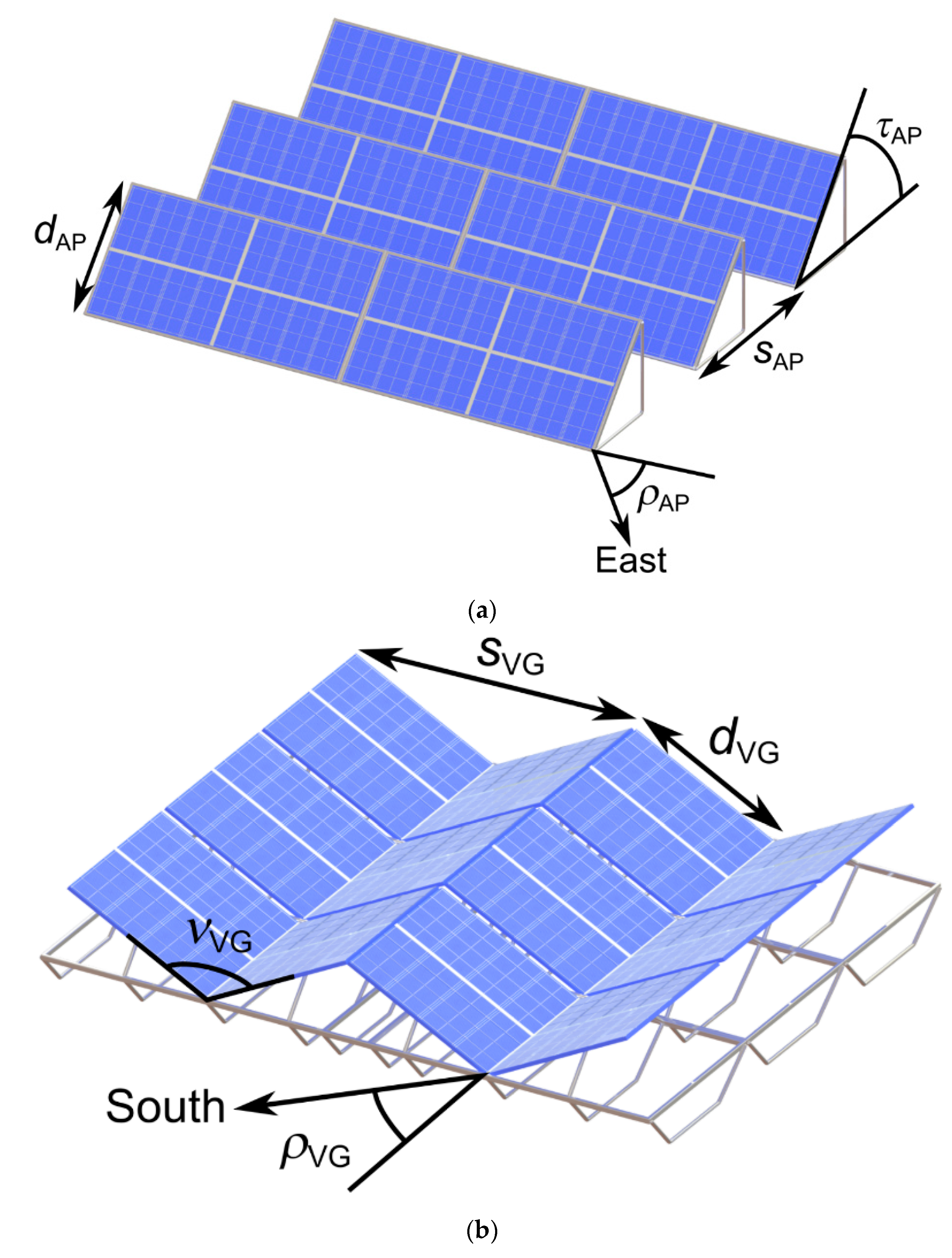
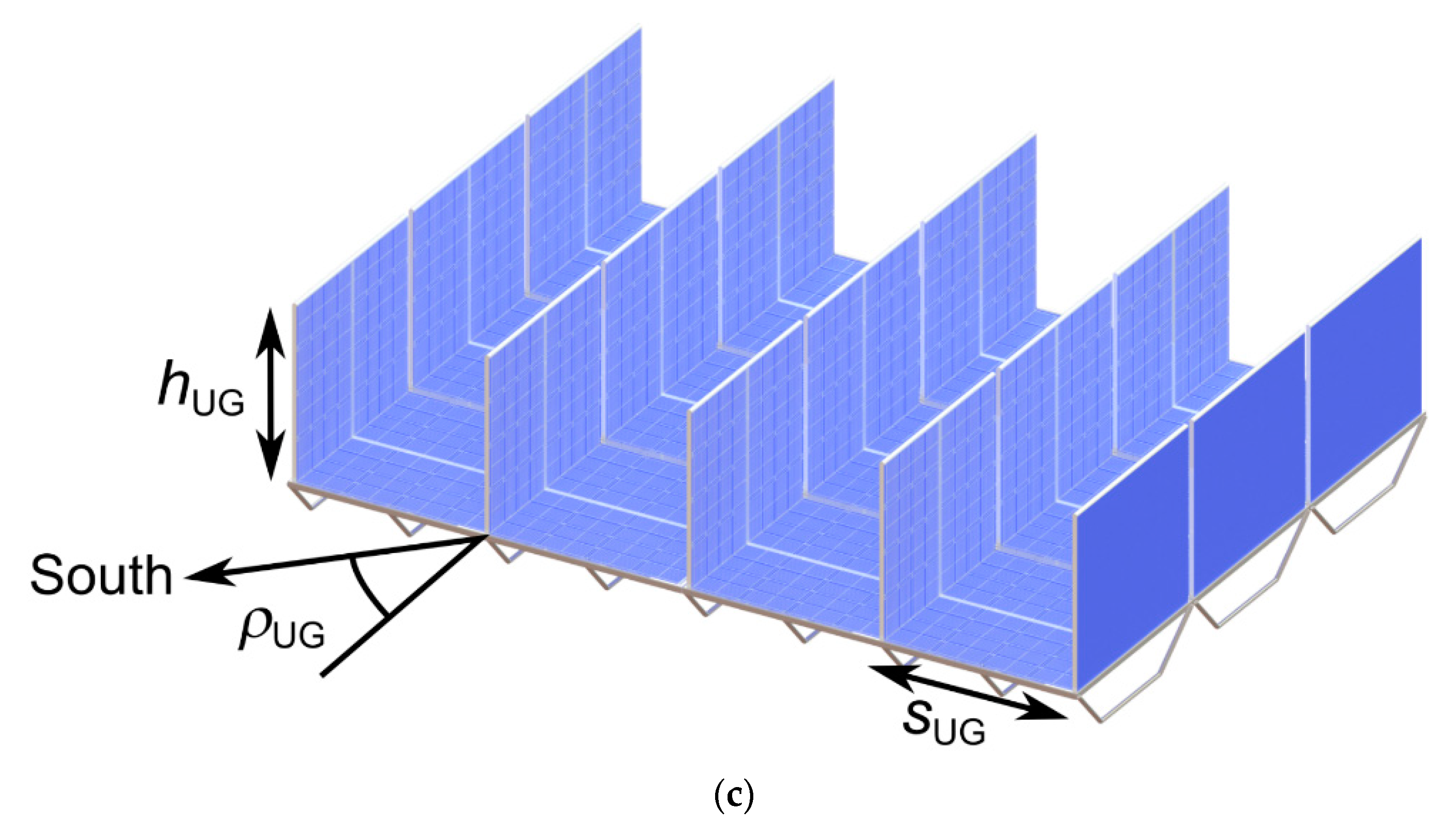
2. Solar Array Geometries

The considered solar arrays enable scalability in that they can be formed by simple geometric tiling of commercial rectangular PV modules, eliminating manufacturing or customization beyond the norm. Moreover, the arrays can be rastered over a two-dimensional plane to fill any installation area. Figure 2 shows the three solar arrays of interest.

The angled-panel array in Figure 2a is the industry standard for large installations. The array has rows of PV modules with four key geometric parameters: an azimuthal rotation angle of ρ_AP between the rows’ bearing and the (east-west) circle of latitude, a tilt angle of τ_AP above the horizontal, a transverse distance of d_AP across each surface, and a spacing of s_AP between the rows. Such a geometry is relatively straightforward to implement. However, its performance over the course of a day can be subject to issues of shadowing, as seen in [24,25], convective cooling, as introduced in [26] and applied in [27,28,29,30], and time-varying electricity prices, as proposed in this work.

The V-groove array in Figure 2b is a structure known to improve performance of thin-film photovoltaics [31] due to its ability to trap internal reflections. It consists of V-shaped corrugations of PV modules with four key geometric parameters: an azimuthal rotation angle of ρ_VG between the corrugations’ bearing and the (north-south) line of longitude, an interior v-angle of ν_VG between the top surfaces, a transverse distance of d_VG across each surface, and a spacing of s_VG = 2d_VGsin(ν_VG/2) between the rows. This array has been popular for tandem solar cells, with differing bandgaps for opposing sides [31,32], as it yields photogenerated charge carriers with less excess kinetic energy and thus greater conversion efficiency. Nonetheless, in this work, we recognize that the V-shaped grooves can also improve light capture during the early- and late-day hours, when electricity prices are the highest, suggesting that it may generate an enhanced value of electricity.

The U-groove array in Figure 2c has rows of walls, with PV modules on the opposing surfaces, on top of a planar surface of PV modules. It is characterized by three key geometric parameters: an azimuthal rotation angle of ρ_UG between the walls’ bearing and the (north-south) line of longitude, a height of h_UG for the walls, and a spacing of s_UG between the walls. To the authors’ best knowledge, such a geometry has not been studied for solar arrays, but it has the potential to broaden the duration of light capture over the course of a day beyond that of the V-groove array. This is because the U-groove array’s bottom effectively captures light for high-angled (midday) illumination, while the walls continue light capture for low-angled (early- and late-day) illumination via internal reflections. Our work weighs the increase in generated value of electricity for this array against its increased cost, with a comparison to the angled-panel and V-groove arrays.

The solar arrays that are compared in this work were first optimized in terms of their geometric parameters. For this optimization, it was recognized that larger arrays, with many PV modules, have an advantage over their counterparts built from fewer PV modules. This is because arrays with greater numbers of PV modules can better adapt to shadowing via blocking diodes that disconnect the shadowed modules. To separate this effect of scale from the inherent performance differences of the arrays, it was necessary to select a standardized scale for comparison. Hence, the minimal size was selected, where each flat surface consists of a single PV module functioning as a single solar cell. The arrays were then optimized and analysed with a set transverse distance (in the case of the angled-panel and V-groove arrays) or set height (in the case of the U-groove array).

3. Analyses

The investigated solar arrays were subjected to experimental, theoretical, and economic analyses, as detailed in the following subsections. The experimental analyses focused on the constituent solar cells in characterizing their time-varying functionality and nonideality in realistic/field deployments. The theoretical analyses quantified the light-capturing ability of these solar cells as applied within the solar arrays. This was done with consideration to all manners of solar illumination, including specular (direct) and diffuse (indirect) incidence as well as the ensuing specular (mirror-like) and diffuse (scattered) reflections within the arrays. The economic analyses then merged the experimental and theoretical findings to define the generated value versus incurred cost for each solar array over a 5-year study under conditions of high solar penetration.

3.1. Experimental Analyses (of the Constituent Solar Cells)

The experimental analyses described here were used to characterize silicon solar cells under realistic/field conditions, with thought to their time-varying functionality and nonideality via self-heating, peripheral wiring, etc. The solar cells were monocrystalline silicon with an efficiency of 18% and area of 76.2 × 76.2 mm². They had alkaline-etched surface texturing and were capped by an ethylene vinyl acetate-film encapsulant and a 3-mm-thick low-iron-glass protective layer. This was done to mimic the packaging of solar cells within a PV module. (Such capping protects the solar cells but can lead to specular reflections within the array and self-heating of the solar cells). The solar cells were tested in an assortment of array types and orientations on the rooftop of a four-storey building in the locale of 49.939° N, 119.394° W. The elevated setting was chosen to yield characterizations with minimal obstructions over the full course of a day.

Current versus voltage measurements were acquired by an electrical circuit at 5-min intervals. For each measurement, the solar cell’s load resistance was varied and its current-voltage (I–V) curves were recorded, with an open-circuit state between the measurements. A total of 276 I–V curves were collected, with the results used to define the underlying parameters of the solar cells. The I–V characteristics were analysed according to a simplified form [33] of the double-diode solar cell equation [34], which can be cast in the form of the semi-empirical implicit relation

$$\begin{array}{l}{J}_{\mathrm{pv}}(\theta )={\displaystyle \underset{300\mathrm{nm}}{\overset{1200\mathrm{nm}}{\int }}{n}_{\lambda }{R}_{\mathsf{\lambda }}(\lambda )\hspace{0.17em}S(\lambda ,\mathrm{AM}(\theta ))}\hspace{0.17em}d\lambda -J_{\mathrm{sat}1}\exp (\hspace{0.17em}(V+J_{\mathrm{pv}}{R}_{\mathrm{s}})/V_{\mathrm{T}}\hspace{0.17em})\\ \hspace{1em}\hspace{1em}\hspace{1em}\hspace{1em}-J_{\mathrm{sat}2}\exp (\hspace{0.17em}(V+J_{\mathrm{pv}}{R}_{\mathrm{s}})/n_{\mathrm{d}}{V}_{\mathrm{T}}\hspace{0.17em})-(V-J_{\mathrm{pv}}{R}_{\mathrm{s}})/R_{\mathrm{sh}}.\end{array}$$

(1)

Here, J_pv(θ) is the measured current density at a solar zenith angle of θ, V is the measured voltage, and V_T is the junction thermal voltage. The first term defines the photocurrent density as a product of a responsivity scaling factor, n_λ, the normalized spectral responsivity, R_λ(λ), as a function of the wavelength, λ, and the spectral irradiance distribution, S(λ,AM(θ)), as a function of the wavelength, λ, and air mass (AM) at the given solar zenith angle, AM(θ). The spectral responsivity of the silicon solar cells was estimated from several sources [35,36,37,38] and applied here as a wavelength-dependent quantity. This was done to better characterize the high-value early- and late-day light, for which the long atmospheric path lengths shift the spectrum away from the standard AM1.5 spectrum [39]. The second term contains the first saturation current density, J_sat1, and series resistance, R_s. The third term contains the second saturation current density, J_sat2, and diode ideality factor, n_d, which is assumed to be 2 as a common assumption [40]. The fourth term contains the shunt resistance, R_sh.

The experimental I–V characteristics were fit to the above equation to yield values for the five parameters. Fitting for the responsivity scaling factor gives n_r = 0.742. Fitting for the first saturation current density suggests that the temperature of the solar cell is above the ambient. We attributed this to self-heating at a rate of 25 °C/(1000 W/m²), in accordance with [41]. This J_sat1 is the result of bulk and surface recombination in the solar cell, which depends upon the minority charge carrier density and thus scales in proportion to the square of the intrinsic charge-carrier density. The intrinsic charge-carrier varies with temperature, T, according to T^3/2exp(–E_g/2k_BT), where E_g = 1.1 eV is the bandgap energy of silicon and k_B is Boltzmann’s constant, and so J_sat1 follows T³exp(–E_g/k_BT) [42]. Such a relation gives a first saturation current density of J_sat1 = 471 fA/cm² at a solar cell temperature of 25 °C, which is comparable to values in the literature [40]. Fitting for the second saturation current density, J_sat2, suggests that the I-V characteristics have only a weak dependence on it, in that it shows only a slight rise at midday due to increased temperature. This J_sat2 is the result of trap-assisted recombination in the junction, with the rate of recombination proportional to the product of intrinsic charge-carrier density and temperature, and so J_sat2 follows T^5/2exp(–E_g/2k_BT). The temperature dependence seen here is weaker than that of the first saturation current density, but it is still important [43]. A second saturation current density of J_sat2 = 15.4 nA/cm² is extracted here for a temperature of 25 °C. This is comparable to the values seen in the literature and is attributed to the strong edge recombination of commercial silicon solar cells [40]. Fitting for the series resistance yields large values that are dominated by the peripheral wiring. Thus, a closer to average [39], but still large, value of R_s = 3 Ω·cm² is used here. Fitting for the shunt resistance yields R_sh = 37.74 kΩ·cm², which is in accordance with the literature [40].

Ultimately, the generated electrical power from the solar arrays will result from the optoelectronic conversion of the constituent solar cells, as defined here, and the captured optical power of the solar cells in the assembled arrays, as given in the next subsection.

3.2. Theoretical Analyses (of the Assembled Solar Arrays)

The theoretical analyses put forward here target explicit expressions for the captured optical power densities of the solar arrays. The metric of captured optical power density is defined as the total optical power transmitted into the solar cells within each array per unit area on the horizontal surface, i.e., installation area. The expressions are derived from first principles, to avoid common assumptions that can lose validity at large solar zenith angles. This is done while considering all manners of angle-dependent solar illumination, including specular (direct) and diffuse (indirect) incidence as well as the ensuing specular (mirror-like) and diffuse (scattered) reflections within the arrays. Aspects related to the specular illumination can be seen in a prior publication of the authors [44], while the full analytical details can be seen in one author’s thesis [45].

Specular illumination comes about from direct incidence of sunlight, and it is characterized in this work for the sun at a solar azimuth angle of ϕ and solar zenith angle of θ. The AM value for such illumination is defined by the relation [46]

$$\mathrm{AM}(\theta )=\frac{1{.002432\cos }^2\theta +0.148386\cos \theta +0.0096467}{{\cos }^3\theta +0{.149864\cos }^2\theta +0.0102963\cos \theta +0.000303978}.$$

(2)

An empirical relation is used here, in lieu of the common approximation of AM(θ) ≈ secθ, to quantify effects of the Earth’s curvature and the refraction of its atmosphere at large solar zenith angles, when the sun is near the horizon. These large angles are important to this study given the higher electricity prices, and the potential for increased generated value, at the early- and late-day hours. The specular solar irradiance is then defined as the directly incident solar power per unit area over the horizontal surface, as defined by

$$I_{\mathrm{solar}}^{\mathrm{spec}}(\theta )=\hspace{0.17em}{\displaystyle \underset{300\mathrm{nm}}{\overset{1200\mathrm{nm}}{\int }}S(\lambda ,\mathrm{AM}(\theta ))\hspace{0.17em}\hspace{0.17em}\cos \theta \hspace{0.17em}d\lambda }.$$

(3)

Here, the solar power per unit area normal to the illumination and per unit wavelength, λ, is defined by the solar irradiance distribution S(λ,AM(θ)) = S(λ,AM = 1.5)^{(AM(θ)/1.5)/}S(λ,AM = 0.0)^{(AM(θ)/1.5−1)}, where S(λ,AM = 1.5) and S(λ,AM = 0.0) are the well-known solar irradiance distributions of the AM1.5 and AM0.0 spectra, respectively [47,48]. The cosθ appears here due to the differing orientations of unit area in the specular solar irradiance and S(λ,AM(θ)). The specular solar irradiance is applied here with wavelength dependence embedded in it, although the analyses can also be carried out using the wavelength-dependent S(λ,AM(θ)), with integration over this distribution at the end. Such an approach enables the use of a wavelength-dependent reflectance. Nonetheless, we have found that both approaches yield similar results, and so the simpler formulation with the specular solar irradiance is presented in this section.

Diffuse illumination comes about from indirect incidence of sunlight, due to scattering in the atmosphere, and it is defined in this work by the diffuse solar irradiance. This irradiance quantifies the diffuse solar power incident per unit area over the horizontal surface and is defined by

$$I_{\mathrm{solar}}^{\mathrm{diff}}(\theta )=\{\begin{array}{ll}(39.78\hspace{0.17em}{\mathrm{W}/\mathrm{m}}^2){\cos }^{0.35}\theta +(79.3059\hspace{0.17em}{\mathrm{W}/\mathrm{m}}^2){\cos }^{0.66}\theta ,& \theta \le 1.53\hspace{0.17em}\hspace{0.17em}\mathrm{rad},\\ (1200.2\hspace{0.17em}{\mathrm{W}/\mathrm{m}}^2){(1.64\hspace{0.17em}\mathrm{rad}-\theta )}^{1.8},& 1.53\hspace{0.17em}\hspace{0.17em}\mathrm{rad}<\theta \le 1.64\hspace{0.17em}\hspace{0.17em}\mathrm{rad},\\ 0,& \theta >1.64 \mathrm{rad}.\end{array}$$

(4)

This piecewise function is formed by fitting empirical data for diffuse light at small solar zenith angles [49] to empirical data for diffuse light at large solar zenith angles [50]. This better quantifies the pronounced effects of scattering during the early- and late-day hours.

Ultimately, the specular and diffuse solar irradiance can be applied to each array to characterize its light-capturing ability for specular (direct) and diffuse (indirect) incidence as well as its ensuing specular (mirror-like) and diffuse (scattered) reflections. This is done with the flat-panel array as a benchmark for comparison. The specular, diffuse, and total captured optical power densities of this flat-panel array are defined simply by

$$P_{\mathrm{FP}}^{\mathrm{cap},\mathrm{spec}}(\theta )=I_{\mathrm{solar}}^{\mathrm{spec}}(\theta )(1-R),$$

(5)

$$P_{\mathrm{FP}}^{\mathrm{cap},\mathrm{diff}}(\theta )=I_{\mathrm{solar}}^{\mathrm{diff}}(\theta )(1-R), \mathrm{and}$$

(6)

$$P_{\mathrm{FP}}^{\mathrm{cap}}(\theta )=P_{\mathrm{FP}}^{\mathrm{cap},\mathrm{spec}}(\theta )+P_{\mathrm{FP}}^{\mathrm{cap},\mathrm{diff}}(\theta ),$$

(7)

respectively. Here, R is the reflectance of the PV module’s upper surface, assuming negligible grid coverage by the contacts (which typically cover only a few percent of the surface area). In the next subsections, the specular, diffuse, and total captured optical power densities are computed for the more complex angled-panel, V-groove, and U-groove arrays.

3.2.1. Angled-Panel Array

We first consider the captured optical power density of the angled-panel array for solar illumination via specular (direct) and diffuse (indirect) incidence as well as ensuing diffuse (scattered) reflections within the array. Specular (mirror-like) reflections are not considered here because it is assumed that the PV modules have matte backings with little luster. The modules are implemented in this angled-panel array with a rotation angle of ρ_AP, tilt angle of τ_AP, transverse distance of d_AP, and spacing of s_AP, as shown in Figure 2a.

Specular illumination of the angled-panel array manifests from direct incidence of sunlight onto the front of its modules. The direct solar illumination is characterized by a vector oriented along the azimuth angle of ϕ and zenith angle of θ. The projection of this vector into the plane of incidence, passing through the (north-south) line of longitude and zenith, lies at an angle of

$${\gamma }_{\mathrm{AP}}(\varphi ,\theta )=\arctan (\tan \theta \cos \varphi )$$

(8)

with respect to the zenith. We use this angle to find the total optical power incident on the front surfaces of the modules per unit area over the horizontal surface. It can be shown that the resulting specular incident optical power density of the angled-panel array is

$$\begin{array}{l}{P}_{\mathrm{AP}}^{\mathrm{inc},\mathrm{spec}}(\varphi ,\theta )=\\ \{\begin{array}{c}\begin{array}{l}{I}_{\mathrm{solar}}^{\mathrm{spec}}(\theta )(\tan ({\gamma }_{\mathrm{AP}}(\varphi ,\theta ))\sin ({\tau }_{\mathrm{AP}})+\cos ({\tau }_{\mathrm{AP}}))d_{\mathrm{AP}}/s_{\mathrm{AP}},\hspace{0.17em}\\ \hspace{1em}{\tau }_{\mathrm{AP}}-\frac{\pi }{2}<{\gamma }_{\mathrm{AP}}(\varphi ,\theta )<{\tau }_{\mathrm{AP}}-\frac{\pi }{2}+\arccos \left(\frac{2d_{\mathrm{AP}}^2+s_{\mathrm{AP}}^2-2d_{\mathrm{AP}}{s}_{\mathrm{AP}}\cos ({\tau }_{\mathrm{AP}})}{2d_{\mathrm{AP}}\sqrt{d_{\mathrm{AP}}^2+s_{\mathrm{AP}}^2-2d_{\mathrm{AP}}{s}_{\mathrm{AP}}\cos ({\tau }_{\mathrm{AP}})}}\right),\\ I_{\mathrm{solar}}^{\mathrm{spec}}(\theta ),\\ \hspace{1em}{\tau }_{\mathrm{AP}}-\frac{\pi }{2}+\arccos \left(\frac{2d_{\mathrm{AP}}^2+s_{\mathrm{AP}}^2-2d_{\mathrm{AP}}{s}_{\mathrm{AP}}\cos ({\tau }_{\mathrm{AP}})}{2d_{\mathrm{AP}}\sqrt{d_{\mathrm{AP}}^2+s_{\mathrm{AP}}^2-2d_{\mathrm{AP}}{s}_{\mathrm{AP}}\cos ({\tau }_{\mathrm{AP}})}}\right)\le {\gamma }_{\mathrm{AP}}(\varphi ,\theta )<\frac{\pi }{2},\hspace{0.17em}\hspace{0.17em}\hspace{0.17em}\hspace{0.17em}\hspace{0.17em}\hspace{0.17em}\hspace{0.17em}\hspace{0.17em}\hspace{0.17em}\hspace{0.17em}\end{array}\end{array}\end{array}$$

(9)

where the piecewise cases correspond to full and partial illumination on the front of the modules. The specular captured optical power density of the angled-panel array is then

$$P_{\mathrm{AP}}^{\mathrm{cap},\mathrm{spec}}(\varphi ,\theta )=(1-R)P_{\mathrm{AP}}^{\mathrm{inc},\mathrm{spec}}(\varphi ,\theta ).$$

(10)

Diffuse illumination of the angled-panel array manifests from indirect incidence of sunlight in the atmosphere onto the front of its modules and scattered reflections within the array. The reflectance on the front surface of the modules is R, as defined in the prior section, and the reflectance on the ground and matte backing of the modules is taken to be R′ = 0.75, in accordance with [51].

We enumerate the internal reflections by the integer n and consider thin strips of area running along the length of the array, with each having a width of δ. On the front surface, back surface, and ground, each strip is indexed by i, j, and k, respectively, with each located at a distance off the PV-module-to-ground contact point of d_i, d_j, and d_k, respectively. It can be shown that prior to any reflections, n = 0, the angled-panel array has diffuse incident optical power densities on the front surface, back surface, and ground of

$$P_{\mathrm{AP},\mathrm{front}}^{\mathrm{inc},\mathrm{diff}}(\varphi ,\theta ;n=0,i)=\frac{I_{\mathrm{solar}}^{\mathrm{diff}}(\theta )\delta }{2s_{\mathrm{AP}}}\left(1-\frac{h_{\mathrm{AP}}-d_i-s_{\mathrm{AP}}\cos ({\tau }_{\mathrm{AP}})}{\sqrt{{(h_{\mathrm{AP}}-d_i)}^2+s_{\mathrm{AP}}^2-2(h_{\mathrm{AP}}-d_i)s_{\mathrm{AP}}\cos ({\tau }_{\mathrm{AP}})}}\right),$$

(11)

$$P_{\mathrm{AP},\mathrm{back}}^{\mathrm{inc},\mathrm{diff}}(\varphi ,\theta ;n=0,j)=\frac{I_{\mathrm{solar}}^{\mathrm{diff}}(\theta )\delta }{2s_{\mathrm{AP}}}\left(1-\frac{h_{\mathrm{AP}}-d_j+s_{\mathrm{AP}}\cos ({\tau }_{\mathrm{AP}})}{\sqrt{{(h_{\mathrm{AP}}-d_j)}^2+s_{\mathrm{AP}}^2+2(h_{\mathrm{AP}}-d_j)s_{\mathrm{AP}}\cos ({\tau }_{\mathrm{AP}})}}\right), \mathrm{and}$$

(12)

$$\begin{array}{l}{P}_{\mathrm{AP},\mathrm{ground}}^{\mathrm{diff},\mathrm{inc}}(\varphi ,\theta ;n=0,k)=\\ \hspace{0.17em}\frac{I_{\mathrm{solar}}^{\mathrm{diff}}(\theta )\delta }{2s_{\mathrm{UG}}}\hspace{0.17em}(\hspace{0.17em}\hspace{0.17em}\sin \left(\arctan \left(\frac{d_k+h_{\mathrm{AP}}\cos ({\tau }_{\mathrm{AP}})}{h_{\mathrm{AP}}\sin ({\tau }_{\mathrm{AP}})}\right)\right)-\sin \left(\arctan \left(\frac{d_k-s_{\mathrm{UG}}+h_{\mathrm{AP}}\cos ({\tau }_{\mathrm{AP}})}{h_{\mathrm{AP}}\sin ({\tau }_{\mathrm{AP}})}\right)\right)\hspace{0.17em}\hspace{0.17em}),\end{array}$$

(13)

respectively. Subsequent diffuse reflections on the surfaces are then characterized by Lambertian scatter patterns [52], which are methodically tracked as cascaded projections off of each surface and onto the neighbouring surfaces. It can be shown that, following n reflections, the angled-panel array has diffuse incident optical power densities on the front surface, back surface, and ground of

$$\begin{array}{l}{P}_{\mathrm{AP},\mathrm{front}}^{\mathrm{diff},\mathrm{inc}}(\varphi ,\theta ;n>0,i)=\\ \hspace{0.17em}{\displaystyle \sum _{k=1}^{s_{\mathrm{AP}}/\delta }{P}_{\mathrm{AP},\mathrm{ground}}^{\mathrm{diff},\mathrm{inc}}(\varphi ,\theta ;n-1,k)\frac{R’}{2}\left(\begin{array}{l}\frac{d_i+(d_k-\delta /2)\cos ({\tau }_{\mathrm{AP}})}{\sqrt{d_i^2+{(d_k-\delta /2)}^2+2d_i(d_k-\delta /2)\cos ({\tau }_{\mathrm{AP}})}}\\ -\frac{d_i+(d_k+\delta /2)\cos ({\tau }_{\mathrm{AP}})}{\sqrt{d_i^2+{(d_k+\delta /2)}^2+2d_i(d_k+\delta /2)\cos ({\tau }_{\mathrm{AP}})}}\end{array}\right)}\\ \hspace{0.17em}+{\displaystyle \sum _{j=1}^{h_{\mathrm{AP}}/\delta }{P}_{\mathrm{AP},\mathrm{back}}^{\mathrm{diff},\mathrm{inc}}(\varphi ,\theta ;n-1,j)\hspace{0.17em}\hspace{0.17em}\frac{R’}{2}\hspace{0.17em}\hspace{0.17em}\left(\begin{array}{l}\sin \left(\arctan \left(\frac{d_i-d_j+\delta /2+s_{\mathrm{AP}}\cos ({\tau }_{\mathrm{AP}})}{s_{\mathrm{AP}}\sin ({\tau }_{\mathrm{AP}})}\right)\right)\\ -\sin \left(\arctan \left(\frac{d_i-d_j-\delta /2+s_{\mathrm{AP}}\cos ({\tau }_{\mathrm{AP}})}{s_{\mathrm{AP}}\sin ({\tau }_{\mathrm{AP}})}\right)\right)\end{array}\right)},\end{array}$$

(14)

$$\begin{array}{l}{P}_{\mathrm{AP},\mathrm{back}}^{\mathrm{diff},\mathrm{inc}}(\varphi ,\theta ;n>0,j)=\\ {\displaystyle \sum _{k=1}^{s_{\mathrm{AP}}/\delta }{P}_{\mathrm{AP},\mathrm{ground}}^{\mathrm{diff},\mathrm{inc}}(\varphi ,\theta ;n-1,k)\frac{R’}{2}\left(\begin{array}{l}\frac{d_j-(s_{\mathrm{AP}}-d_k-\delta /2)\cos ({\tau }_{\mathrm{AP}})}{\sqrt{d_j^2+{(s_{\mathrm{AP}}-d_k-\delta /2)}^2-2d_j(s_{\mathrm{AP}}-d_k-\delta /2)\cos ({\tau }_{\mathrm{AP}})}}\\ -\frac{d_j-(s_{\mathrm{AP}}-d_k+\delta /2)\cos ({\tau }_{\mathrm{AP}})}{\sqrt{d_j^2+{(s_{\mathrm{AP}}-d_k+\delta /2)}^2-2d_j(s_{\mathrm{AP}}-d_k+\delta /2)\cos ({\tau }_{\mathrm{AP}})}}\end{array}\right)}\\ +{\displaystyle \sum _{i=1}^{h_{\mathrm{AP}}/\delta }{P}_{\mathrm{AP},\mathrm{front}}^{\mathrm{diff},\mathrm{inc}}(\varphi ,\theta ;n-1,i)\hspace{0.17em}\hspace{0.17em}\frac{R}{2}\hspace{0.17em}\hspace{0.17em}\left(\begin{array}{l}\sin \left(\arctan \left(\frac{d_i-d_j+\delta /2+s_{\mathrm{AP}}\cos ({\tau }_{\mathrm{AP}})}{s_{\mathrm{AP}}\sin ({\tau }_{\mathrm{AP}})}\right)\right)\\ -\sin \left(\arctan \left(\frac{d_i-d_j-\delta /2+s_{\mathrm{AP}}\cos ({\tau }_{\mathrm{AP}})}{s_{\mathrm{AP}}\sin ({\tau }_{\mathrm{AP}})}\right)\right)\end{array}\right)},\hspace{0.17em}\hspace{0.17em}\hspace{0.17em}\hspace{0.17em}\mathrm{and}\end{array}$$

(15)

$$\begin{array}{l}{P}_{\mathrm{AP},\mathrm{ground}}^{\mathrm{diff},\mathrm{inc}}(\varphi ,\theta ;n>0,k)=\\ \hspace{0.17em}\hspace{0.17em}\hspace{0.17em}\hspace{0.17em}{\displaystyle \sum _{i=1}^{h_{\mathrm{AP}}/\delta }{P}_{\mathrm{AP},\mathrm{front}}^{\mathrm{diff},\mathrm{inc}}(\varphi ,\theta ;n-1,i)\frac{R}{2}\left(\begin{array}{l}\frac{d_k+(d_i-\delta /2)\cos ({\tau }_{\mathrm{AP}})}{\sqrt{d_k^2+{(d_i-\delta /2)}^2+2d_k(d_i-\delta /2)\cos ({\tau }_{\mathrm{AP}})}}\\ -\frac{d_k+(d_i+\delta /2)\cos ({\tau }_{\mathrm{AP}})}{\sqrt{d_k^2+{(d_i+\delta /2)}^2+2d_k(d_i+\delta /2)\cos ({\tau }_{\mathrm{AP}})}}\end{array}\right)}\\ +{\displaystyle \sum _{j=1}^{h_{\mathrm{AP}}/\delta }{P}_{\mathrm{AP},\mathrm{back}}^{\mathrm{diff},\mathrm{inc}}(\varphi ,\theta ;n-1,j)\frac{R’}{2}\left(\begin{array}{l}\frac{s_{\mathrm{AP}}-d_k-(d_j-\delta /2)\cos ({\tau }_{\mathrm{AP}})}{\sqrt{{(s_{\mathrm{AP}}-d_k)}^2+{(d_j-\delta /2)}^2-2(s_{\mathrm{AP}}-d_k)(d_j-\delta /2)\cos ({\tau }_{\mathrm{AP}})}}\\ -\frac{s_{\mathrm{AP}}-d_k-(d_j+\delta /2)\cos ({\tau }_{\mathrm{AP}})}{\sqrt{{(s_{\mathrm{AP}}-d_k)}^2+{(d_j+\delta /2)}^2-2(s_{\mathrm{AP}}-d_k)(d_j+\delta /2)\cos ({\tau }_{\mathrm{AP}})}}\end{array}\right)},\end{array}$$

(16)

respectively. These diffuse incident optical power densities are computed for all consecutive reflections throughout the structure until they have been reduced by five orders of magnitude. The optical power densities, having been captured by all of the strips over the front surface, indexed by i, for all reflections, and indexed by n, are then summed to define the diffuse captured optical power density of the angled-panel array as

$$P_{\mathrm{AP}}^{\mathrm{cap},\mathrm{diff}}(\varphi ,\theta )={\displaystyle \sum _{i=1}^{h_{\mathrm{UG}}/\delta }{\displaystyle \sum _{n=0}^{\infty }(1-R)}{P}_{\mathrm{AP},\mathrm{front}}^{\mathrm{inc},\mathrm{diff}}(\varphi ,\theta ;n,i)}\hspace{0.17em}.$$

(17)

Finally, the total captured optical power density of the angled-panel array is computed by

$$P_{\mathrm{AP}}^{\mathrm{cap}}(\varphi ,\theta )=P_{\mathrm{AP}}^{\mathrm{cap},\mathrm{spec}}(\varphi ,\theta )+P_{\mathrm{AP}}^{\mathrm{cap},\mathrm{diff}}(\varphi ,\theta ).$$

(18)

3.2.2. V-Groove Array

We next consider the captured optical power density of the V-groove array for solar illumination via specular (direct) and diffuse (indirect) incidence and the ensuing specular (mirror-like) and diffuse (scattered) reflections within the array. The PV modules are implemented in the V-groove array with a rotation angle of ρ_VG, an interior v-angle of ν_VG, a transverse distance of d_VG, and a spacing of s_VG = 2d_VGsin(ν_VG/2), as shown in Figure 2b.

Specular illumination of the V-groove array manifests from direct incidence of sunlight onto the front of its modules and mirror-like reflections within the array. As before, the direct solar illumination is characterized by a vector oriented along the azimuth angle of ϕ and zenith angle of θ. However, the distinct east- and west-facing sides of the V-groove array here demand that the projections of this vector into the plane of incidence, passing through the (east-west) line of latitude and zenith, be characterized by distinct angles of γ_VG,east(ϕ,θ;n) and γ_VG,west(ϕ,θ;n), respectively. Likewise, the east- and west-facing sides have distances from the vertex to the lower edges of incident illumination of ℓ_VG,east(ϕ,θ;n) and ℓ_VG,west(ϕ,θ;n), respectively, and distances from the vertex to the upper edges of incident illumination of u_VG,east(ϕ,θ;n) and u_VG,west(ϕ,θ;n), respectively, where n is the number of reflections. By methodically tracking the cascaded incidence, reflection, and projection of light within the V-groove array, we can state

$${\gamma }_{\mathrm{VG},\mathrm{east}/\mathrm{west}}^{}(\varphi ,\theta ;n)=\{\begin{array}{c}(+/-)\hspace{0.17em}\hspace{0.17em}\arctan (\tan \theta \sin \varphi ),\hspace{0.17em}\hspace{0.17em}\hspace{0.17em}\hspace{0.17em}\hspace{0.17em}\hspace{0.17em}\hspace{0.17em}\hspace{0.17em}\hspace{0.17em}\hspace{0.17em}\hspace{0.17em}\hspace{0.17em}\hspace{0.17em}\hspace{0.17em}\hspace{0.17em}\hspace{0.17em}\hspace{0.17em}n=0,\\ {\gamma }_{\mathrm{VG},\mathrm{west}/\mathrm{east}}^{}(\varphi ,\theta ;n-1)+{\nu }_{\mathrm{VG}},\hspace{0.17em}\hspace{0.17em}\hspace{0.17em}\hspace{0.17em}\hspace{0.17em}\hspace{0.17em}\hspace{0.17em}\hspace{0.17em}\hspace{0.17em}\hspace{0.17em}\hspace{0.17em}n>0.\end{array}$$

(19)

$$\begin{array}{l}{\ell }_{\mathrm{VG},\mathrm{east}/\mathrm{west}}^{}(\varphi ,\theta ;n)=\\ \{\begin{array}{ll}{d}_{\mathrm{VG}}\max \left(\frac{\sin (\hspace{0.17em}{\gamma }_{\mathrm{VG},\mathrm{east}/\mathrm{west}}^{}(\varphi ,\theta ;n)\hspace{0.17em}\hspace{0.17em}-{\nu }_{\mathrm{VG}})}{\sin (\pi -\hspace{0.17em}\hspace{0.17em}{\gamma }_{\mathrm{VG},\mathrm{east}/\mathrm{west}}^{}(\varphi ,\theta ;n)\hspace{0.17em}\hspace{0.17em}-{\nu }_{\mathrm{VG}})},0\right),& n=0,\hspace{1em}\\ {\ell }_{\mathrm{VG},\mathrm{west}/\mathrm{east}}^{}(\varphi ,\theta ;n-1)\frac{\sin (\hspace{0.17em}\hspace{0.17em}\hspace{0.17em}{\gamma }_{\mathrm{VG},\mathrm{east}/\mathrm{west}}^{}(\varphi ,\theta ;n)\hspace{0.17em}-{\nu }_{\mathrm{VG}}/2\hspace{0.17em})}{\sin (\hspace{0.17em}\pi -\hspace{0.17em}\hspace{0.17em}{\gamma }_{\mathrm{VG},\mathrm{east}/\mathrm{west}}^{}(\varphi ,\theta ;n)\hspace{0.17em}-{\nu }_{\mathrm{VG}}/2\hspace{0.17em})},& n>0,\hspace{1em}\hspace{1em}\end{array}\mathrm{and}\end{array}$$

(20)

$$\begin{array}{l}{u}_{\mathrm{VG},\mathrm{east}/\mathrm{west}}^{}(\varphi ,\theta ;n)=\\ \{\begin{array}{ll}{d}_{\mathrm{VG}},& n=0,\\ u_{\mathrm{VG},\mathrm{west}/\mathrm{east}}^{}(\varphi ,\theta ;n-1)\hspace{0.17em}\frac{\sin (\hspace{0.17em}{\gamma }_{\mathrm{VG},\mathrm{east}/\mathrm{west}}^{}(\varphi ,\theta ;n)-{\nu }_{\mathrm{VG}}/2\hspace{0.17em})}{\sin (\hspace{0.17em}\pi -{\gamma }_{\mathrm{VG},\mathrm{east}/\mathrm{west}}^{}(\varphi ,\theta ;n)-{\nu }_{\mathrm{VG}}/2\hspace{0.17em})},& n>0.\end{array}\end{array}$$

(21)

from which the specular incident and captured optical power densities can be cast as

$$P_{\mathrm{VG},\mathrm{east}/\mathrm{west}}^{\mathrm{inc},\mathrm{spec}}(\varphi ,\theta ;n)\hspace{0.17em}=\{\begin{array}{c}\begin{array}{l}{I}_{\mathrm{solar}}^{\mathrm{spec}}\left(\theta \right)\hspace{0.17em}(u_{\mathrm{VG},\mathrm{east}/\mathrm{west}}^{}(\varphi ,\theta ;n)-{\ell }_{\mathrm{VG},\mathrm{east}/\mathrm{west}}^{}(\varphi ,\theta ;n))\hspace{0.17em}\\ \hspace{1em}\hspace{1em}(\sin ({\nu }_{\mathrm{VG}}/2)+(+/-)\hspace{0.17em}\tan \theta \sin \varphi \cos ({\nu }_{\mathrm{VG}}/2))/s_{\mathrm{VG}},\hspace{0.17em}\hspace{0.17em}n=0,\hspace{0.17em}\end{array}\\ R\hspace{0.17em}{P}_{\mathrm{VG},\mathrm{west}/\mathrm{east}}^{\mathrm{inc},\mathrm{spec}}(\varphi ,\theta ;n-1)/s_{\mathrm{VG}},\hspace{0.17em}\hspace{0.17em}\hspace{0.17em}\hspace{0.17em}\hspace{0.17em}\hspace{0.17em}\hspace{0.17em}\hspace{0.17em}\hspace{0.17em}\hspace{0.17em}\hspace{0.17em}\hspace{0.17em}\hspace{0.17em}\hspace{0.17em}\hspace{0.17em}\hspace{0.17em}\hspace{0.17em}\hspace{0.17em}\hspace{0.17em}\hspace{0.17em}\hspace{0.17em}\hspace{0.17em}\hspace{0.17em}\hspace{0.17em}n>0,\hspace{0.17em}\hspace{0.17em}\end{array}\mathrm{and}$$

(22)

$$P_{\mathrm{VG},\mathrm{east}/\mathrm{west}}^{\mathrm{cap},\mathrm{spec}}(\varphi ,\theta ;n)=(1-R)\hspace{0.17em}{P}_{\mathrm{VG},\mathrm{east}/\mathrm{west}}^{\mathrm{inc},\mathrm{spec}}(\varphi ,\theta ;n).$$

(23)

Here, and in the remainder of this work, the labels ‘·/·’ in the subscripts are instantiated according to the order of their arguments. Thus, the expressions above can be evaluated for the east-facing side (as the first argument) or west-facing side (as the second argument) using the same order of arguments on each expression’s right hand side. This is done with the operator ‘(+/−)’ assigning ‘+’ for the first argument or ‘−’ for the second argument. The operator ‘max(·,·)’ returns the greater of its two arguments. The stepping through n reflections is carried out while testing for a condition in which the incidence on a given side of the array extends above its upper edge, i.e., u_VG,east/west(ϕ,θ;n) > d_VG. When this occurs, the upper edge of the illuminated area is truncated at u_VG,east/west(ϕ,θ;n) = d_VG and the specular incident optical power density is scaled to

$$P_{\mathrm{VG},\mathrm{east}/\mathrm{west}}^{\mathrm{inc},\mathrm{spec}}(\varphi ,\theta ;n)=P_{\mathrm{VG},\mathrm{east}/\mathrm{west}}^{\mathrm{inc},\mathrm{spec}}(\varphi ,\theta ;n)’\hspace{0.17em}\hspace{0.17em}\frac{d_{\mathrm{VG}}-{\ell }_{\mathrm{VG},\mathrm{east}/\mathrm{west}}^{}(\varphi ,\theta ;n)}{u_{\mathrm{VG},\mathrm{east}/\mathrm{west}}^{}(\varphi ,\theta ;n)\hspace{0.17em}’-{\ell }_{\mathrm{VG},\mathrm{east}/\mathrm{west}}^{}(\varphi ,\theta ;n)},$$

(24)

where the primed variables denote the unscaled variables. Stepping through n reflections continues until any one of these three conditions is met: the reflected light travels away from the opposing side of the V-groove array, i.e., γ_VG,east/west(ϕ,θ;n) + 0.5ν_VG > π; the reflected light travels towards but fully misses the opposing side of the V-groove array, i.e., ℓ_VG,east/west(ϕ,θ;n) > d_VG; or the incident optical power density is reduced by nine orders of magnitude. When one of the conditions is met, the power densities on both sides are summed to define the specular captured optical power density of the V-groove array as

$$\begin{array}{l}{P}_{\mathrm{VG}}^{\mathrm{cap},\mathrm{spec}}(\varphi ,\theta )=\hspace{0.17em}{\displaystyle \sum _{n=1,3,5,\hspace{0.17em}\dots }{P}_{\mathrm{VG},\mathrm{east}}^{\mathrm{cap},\mathrm{spec}}(\varphi ,\theta ;n)}+{\displaystyle \sum _{n=0,2,4,\hspace{0.17em}\dots }{P}_{\mathrm{VG},\mathrm{east}}^{\mathrm{cap},\mathrm{spec}}(\varphi ,\theta ;n)}\\ \hspace{0.17em}\hspace{0.17em}\hspace{0.17em}\hspace{0.17em}\hspace{0.17em}\hspace{0.17em}\hspace{0.17em}\hspace{0.17em}\hspace{0.17em}\hspace{0.17em}\hspace{0.17em}\hspace{0.17em}\hspace{0.17em}\hspace{0.17em}\hspace{0.17em}\hspace{0.17em}\hspace{0.17em}\hspace{0.17em}\hspace{0.17em}\hspace{0.17em}\hspace{0.17em}\hspace{0.17em}\hspace{0.17em}\hspace{0.17em}\hspace{0.17em}\hspace{0.17em}\hspace{0.17em}\hspace{0.17em}+{\displaystyle \sum _{n=1,3,5,\hspace{0.17em}\dots }{P}_{\mathrm{VG},\mathrm{west}}^{\mathrm{cap},\mathrm{spec}}(\varphi ,\theta ;n)}+{\displaystyle \sum _{n=0,2,4,\hspace{0.17em}\dots }{P}_{\mathrm{VG},\mathrm{west}}^{\mathrm{cap},\mathrm{spec}}(\varphi ,\theta ;n)}.\end{array}$$

(25)

Diffuse illumination of the V-groove array manifests from indirect incidence of sunlight in the atmosphere onto the front of its modules and scattered reflections within the array. We again consider thin strips of area of width δ running along the length of the array. On the east- or west-facing sides of the array, each strip is indexed by i or j, respectively, and each is located at a distance up from the vertex of d_i or d_j, respectively.

For no reflections, n = 0, the diffuse incident optical power densities on elements i and j are the product of the aforementioned diffuse solar irradiance and the fraction of sky that is visible by each element. It can then be shown that the diffuse incident optical power density on the east- or west-facing sides of the V-groove array is defined by

$$\begin{array}{l}{P}_{\mathrm{VG},\mathrm{east}/\mathrm{west}}^{\mathrm{inc},\mathrm{diff}}(\varphi ,\theta ;n=0,i/j)=\\ \hspace{0.17em}\hspace{0.17em}\hspace{0.17em}\hspace{0.17em}\hspace{0.17em}\frac{I_{\mathrm{solar}}^{\mathrm{diff}}(\theta )\delta }{2s_{\mathrm{VG}}}\hspace{0.17em}\left(1-\frac{(d_{\mathrm{VG}}-d_{i/j})-2{\sin }^2({\nu }_{\mathrm{VG}}/2)d_{\mathrm{VG}}}{\sqrt{{(d_{\mathrm{VG}}-d_{i/j})}^2+4{\sin }^2({\nu }_{\mathrm{VG}}/2)d_{\mathrm{VG}}^2-4(d_{\mathrm{VG}}-d_{i/j}){\sin }^2({\nu }_{\mathrm{VG}}/2)d_{\mathrm{VG}}}}\right),\end{array}$$

(26)

where the labels ‘·/·’ in the subscripts are again instantiated according to their order.

Following n reflections, the diffuse incident optical power density on element i is the summed product of the surface reflectivity, R, the diffuse solar irradiance on element j, and a Lambertian scattering factor that characterizes the diffuse reflection and coupling of light from element j onto element i. Likewise, the diffuse incident optical power density on element j is the summed product of the surface reflectivity, R, the diffuse solar irradiance on element i, and a Lambertian scattering factor that characterizes the diffuse reflection and coupling from element i onto element j. This defines the diffuse incident optical power density of the V-groove array as

$$\begin{array}{l}{P}_{\mathrm{VG},\mathrm{east}/\mathrm{west}}^{\mathrm{inc},\mathrm{diff}}(\varphi ,\theta ;n,i/j)={\displaystyle \sum _{j/i=1}^{d_{\mathrm{VG}}/\delta }\frac{R\hspace{0.17em}{P}_{\mathrm{VG},\mathrm{west}/\mathrm{east}}^{\mathrm{inc},\mathrm{diff}}(\varphi ,\theta ;n-1,j/i)}{2s_{\mathrm{VG}}}}\\ \hspace{0.17em}\hspace{0.17em}\hspace{0.17em}\hspace{0.17em}\hspace{0.17em}\hspace{0.17em}\hspace{0.17em}\hspace{0.17em}\hspace{0.17em}\times (\frac{(d_{\mathrm{VG}}-d_{i/j})-(d_{\mathrm{VG}}-d_{j/i}-\delta /2)\cos ({\nu }_{\mathrm{VG}})}{\sqrt{{(d_{\mathrm{VG}}-d_{i/j})}^2+{(d_{\mathrm{VG}}-d_{j/i}-\delta /2)}^2-2(d_{\mathrm{VG}}-d_{i/j})(d_{\mathrm{VG}}-d_{j/i}-\delta /2)\cos ({\nu }_{\mathrm{VG}})}}\hspace{0.17em}\\ \hspace{0.17em}\hspace{0.17em}\hspace{0.17em}\hspace{0.17em}\hspace{0.17em}\hspace{0.17em}\hspace{0.17em}\hspace{0.17em}\hspace{0.17em}\hspace{0.17em}\hspace{0.17em}\hspace{0.17em}\hspace{0.17em}\hspace{0.17em}-\frac{(d_{\mathrm{VG}}-d_{i/j})-(d_{\mathrm{VG}}-d_{j/i}+\delta /2)\cos ({\nu }_{\mathrm{VG}})}{\sqrt{{(d_{\mathrm{VG}}-d_{i/j})}^2+{(d_{\mathrm{VG}}-d_{j/i}+\delta /2)}^2-2(d_{\mathrm{VG}}-d_{i/j})(d_{\mathrm{VG}}-d_{j/i}+\delta /2)\cos ({\nu }_{\mathrm{VG}})}}).\end{array}$$

(27)

where the labels ‘·/·’ in the subscripts are again instantiated according to their order. The diffuse captured optical power density of the V-groove array is then found by summing the power densities on both sides, according to

$$P_{\mathrm{VG}}^{\mathrm{cap},\mathrm{diff}}(\varphi ,\theta )={\displaystyle \sum _{i=1}^{d_{\mathrm{VG}}/\delta }{\displaystyle \sum _{n=0}^{\infty }(1-R)}}{P}_{\mathrm{VG},\mathrm{east}}^{\mathrm{inc},\mathrm{diff}}(\varphi ,\theta ;n,i)\hspace{0.17em}+\hspace{0.17em}{\displaystyle \sum _{j=1}^{d_{\mathrm{VG}}/\delta }{\displaystyle \sum _{n=0}^{\infty }(1-R)}}{P}_{\mathrm{VG},\mathrm{west}}^{\mathrm{inc},\mathrm{diff}}(\varphi ,\theta ;n,j).$$

(28)

Finally, the total captured optical power density of the V-groove array is calculated by summing the results above from specular and diffuse illumination, by way of

$$P_{\mathrm{VG}}^{\mathrm{cap}}(\varphi ,\theta )=P_{\mathrm{VG}}^{\mathrm{cap},\mathrm{spec}}(\varphi ,\theta )+P_{\mathrm{VG}}^{\mathrm{cap},\mathrm{diff}}(\varphi ,\theta ).$$

(29)

3.2.3. U-Groove Array

We next consider the captured optical power density of the U-groove array for solar illumination via specular (direct) and diffuse (indirect) incidence as well as the ensuing specular (mirror-like) and diffuse (scattered) reflections within the array. The PV modules are implemented in this U-groove array with a rotation angle of ρ_UG, wall height of h_UG, and wall-to-wall spacing of s_UG, as shown in Figure 2c.

Specular illumination of the U-groove array manifests from direct incidence of sunlight onto the front of its modules and mirror-like reflections within the array. As before, the direct solar illumination is characterized by a vector oriented along the azimuth angle of ϕ and zenith angle of θ. The analysis follows that of the V-groove array, but for this array it becomes necessary to distinguish between two cases.

The high-angled-illumination case arises at small solar zenith angles when the bottom of the U-groove array receives direct solar illumination. In this case, the array’s horizontal-to-vertical aspect ratio, N_UG = s_UG/h_UG, meets the condition tanθ|sinϕ| < N_UG, which we can characterize by θ < θ_UG = arctan(N_UG/|sinϕ|). For this case, the specular captured optical power densities of the directly illuminated and shaded walls are given by

$$\begin{array}{l}{P}_{\mathrm{UG},\mathrm{dir}(\mathrm{east}/\mathrm{west})}^{\mathrm{cap},\mathrm{spec}}(\varphi ,\theta <{\theta }_{\mathrm{UG}})=\\ \hspace{1em}\{\begin{array}{ll}{I}_{\mathrm{solar}}^{\mathrm{spec}}(\theta )h_{\mathrm{UG}}(1-R^2)\tan \theta \left|\sin \varphi \right|/s_{\mathrm{UG}},& 2\tan \theta \left|\sin \varphi \right|\hspace{0.17em}\hspace{0.17em}\le N_{\mathrm{UG}}, \mathrm{and}\\ I_{\mathrm{solar}}^{\mathrm{spec}}(\theta )h_{\mathrm{UG}}(1-R)((1-R)\tan \theta |\sin \varphi |+R{N}_{\mathrm{UG}})/s_{\mathrm{UG}},& 2\tan \theta \left|\sin \varphi \right|\hspace{0.17em}\hspace{0.17em}>N_{\mathrm{UG}},\end{array}\end{array}$$

(30)

$$\begin{array}{l}{P}_{\mathrm{UG},\mathrm{shd}(\mathrm{east}/\mathrm{west})}^{\mathrm{cap},\mathrm{spec}}(\varphi ,\theta <{\theta }_{\mathrm{UG}})=\\ \hspace{0.17em}\hspace{0.17em}\hspace{0.17em}\hspace{0.17em}\hspace{0.17em}\{\begin{array}{ll}0,& 2\tan \theta \left|\sin \varphi \right|\hspace{0.17em}\le N_{\mathrm{UG}},\\ I_{\mathrm{solar}}^{\mathrm{spec}}(\theta )h_{\mathrm{UG}}(1-R)R^2\hspace{0.17em}(2\tan \theta |\sin \varphi |-N_{\mathrm{UG}})/s_{\mathrm{UG}},& 2\tan \theta \left|\sin \varphi \right|\hspace{0.17em}\hspace{0.17em}>N_{\mathrm{UG}},\end{array}\end{array}$$

(31)

respectively. Here, ‘dir(east/west)’ instantiates ‘east’ or ‘west’ if the direct solar illumination strikes the east- or west-facing wall, respectively, and ‘shd(east/west)’ instantiates ‘east’ or ‘west’ if shade exists on the east- or west-facing wall, respectively. The results are then summed to define the specular captured optical power density of both walls as

$$P_{\mathrm{UG},\mathrm{walls}}^{\mathrm{cap},\mathrm{spec}}(\varphi ,\theta <{\theta }_{\mathrm{UG}})=P_{\mathrm{UG},\mathrm{east}}^{\mathrm{cap},\mathrm{spec}}(\varphi ,\theta <{\theta }_{\mathrm{UG}})+P_{\mathrm{UG},\mathrm{west}}^{\mathrm{cap},\mathrm{spec}}(\varphi ,\theta <{\theta }_{\mathrm{UG}}),$$

(32)

while the specular captured optical power density of the bottom can be defined simply by

$$P_{\mathrm{UG},\mathrm{bottom}}^{\mathrm{cap},\mathrm{spec}}(\varphi ,\theta <{\theta }_{\mathrm{UG}})=I_{\mathrm{solar}}^{\mathrm{spec}}(\theta )(1-R)(N_{\mathrm{UG}}-\tan \theta |\sin \varphi |(1-R))/N_{\mathrm{UG}}.$$

(33)

The low-angled-illumination case arises at large solar zenith angles when the bottom of the U-groove array does not receive direct solar illumination. Here, the array’s horizontal-to-vertical aspect ratio, N_UG = s_UG/h_UG, ascribes to tanθ|sinϕ| ≥ N_UG and thus θ ≥ θ_UG = arctan(N_UG/|sinϕ|). As the number of reflections can become arbitrarily large here, steps are used to track the cascaded incidence, reflection, and projection of illumination within this array. For each east- and west-facing wall, we define the distance above the ground to the lower and upper edges of incident illumination as ℓ_UG,east/west(ϕ,θ ≥ θ_UG;n) and u_UG,east/west(ϕ,θ ≥ θ_UG;n), respectively. The stepping through n reflections is carried out like that of the V-groove array. However, here we test for a condition where incidence on a wall extends above its upper edge, i.e., u_UG,east/west(ϕ,θ ≥ θ_UG;n) > h_UG, and a condition where incidence on a wall reaches the bottom of the U-groove array, i.e., ℓ_UG,east/west(ϕ,θ ≥ θ_UG;n = r) < 0, where the integer r denotes the reflection at which this occurs. With such definitions, we can state that the specular optical power density on each wall is given by

$$\begin{array}{l}{P}_{\mathrm{UG},\mathrm{east}/\mathrm{west}}^{\mathrm{cap},\mathrm{spec}}(\varphi ,\theta \ge {\theta }_{\mathrm{UG}};n)\\ \hspace{1em}=\{\begin{array}{ll}(1-R)P_{\mathrm{UG},\mathrm{east}/\mathrm{west}}^{\mathrm{inc},\mathrm{spec}}(\varphi ,\theta \ge {\theta }_{\mathrm{UG}};n),& n\ne r,\\ (1-R)P_{\mathrm{UG},\mathrm{east}/\mathrm{west}}^{\mathrm{inc},\mathrm{spec}}(\varphi ,\theta \ge {\theta }_{\mathrm{UG}};n)\tan \theta \left|\sin \varphi \right|& \\ \hspace{1em}\hspace{1em}\times (u_{\mathrm{UG},\mathrm{east}/\mathrm{west}}^{}(\varphi ,\theta \ge {\theta }_{\mathrm{UG}};n)-R{\ell }_{\mathrm{UG},\mathrm{east}/\mathrm{west}}^{}(\varphi ,\theta \ge {\theta }_{\mathrm{UG}};n))/s_{\mathrm{UG}},& n=r.\end{array}\end{array}$$

(34)

For no reflections, n = 0, the above variables are calculated according to

$$u_{\mathrm{UG},\mathrm{east}/\mathrm{west}}^{}(\varphi ,\theta \ge {\theta }_{\mathrm{UG}};n=0)=h_{\mathrm{UG}},$$

(35)

$${\ell }_{\mathrm{UG},\mathrm{east}/\mathrm{west}}^{}(\varphi ,\theta \ge {\theta }_{\mathrm{UG}};n=0)=(1-N_{\mathrm{UG}}/(\tan \theta \left|\sin \varphi \right|))h_{\mathrm{UG}}, \mathrm{and}$$

(36)

$$\begin{array}{ll}{P}_{\mathrm{UG},\mathrm{east}/\mathrm{west}}^{\mathrm{inc},\mathrm{spec}}(\varphi ,\theta \ge {\theta }_{\mathrm{UG}};n=0)=& I_{\mathrm{solar}}^{\mathrm{spec}}(\theta )(u_{\mathrm{UG},\mathrm{east}/\mathrm{west}}^{}(\varphi ,\theta \ge {\theta }_{\mathrm{UG}};n=0)\\ & -{\ell }_{\mathrm{UG},\mathrm{east}/\mathrm{west}}^{}(\varphi ,\theta \ge {\theta }_{\mathrm{UG}};n=0))(\tan \theta \left|\sin \varphi \right|)/s_{\mathrm{UG}}.\end{array}$$

(37)

Following reflections, n > 0, the variables are calculated according to

$$\begin{array}{l}{\ell }_{\mathrm{UG},\mathrm{east}/\mathrm{west}}^{}(\varphi ,\theta \ge {\theta }_{\mathrm{UG}};n)=\\ \hspace{1em}\hspace{1em}\{\begin{array}{ll}+{\ell }_{\mathrm{UG},\mathrm{west}/\mathrm{east}}^{}(\varphi ,\theta \ge {\theta }_{\mathrm{UG}};n-1)-s_{\mathrm{UG}}/(\tan \theta |\sin \varphi |),& n-1<r,\\ -{\ell }_{\mathrm{UG},\mathrm{west}/\mathrm{east}}^{}(\varphi ,\theta \ge {\theta }_{\mathrm{UG}};n-1),& n-1=r,\\ +{\ell }_{\mathrm{UG},\mathrm{west}/\mathrm{east}}^{}(\varphi ,\theta \ge {\theta }_{\mathrm{UG}};n-1)+s_{\mathrm{UG}}/(\tan \theta |\sin \varphi |),& n-1>r,\end{array}\end{array}$$

(38)

$$\begin{array}{l}{u}_{\mathrm{UG},\mathrm{east}/\mathrm{west}}^{}(\varphi ,\theta \ge {\theta }_{\mathrm{UG}};n)=\\ \hspace{0.17em}\hspace{0.17em}\hspace{0.17em}\hspace{0.17em}\hspace{0.17em}\hspace{0.17em}\hspace{0.17em}\hspace{0.17em}\hspace{0.17em}\hspace{0.17em}\hspace{0.17em}\hspace{0.17em}\hspace{0.17em}\hspace{0.17em}\hspace{0.17em}\hspace{0.17em}\hspace{0.17em}\hspace{0.17em}\min ({\ell }_{\mathrm{UG},\mathrm{east}/\mathrm{west}}^{}(\varphi ,\theta \ge {\theta }_{\mathrm{UG}};n)+s_{\mathrm{UG}}/(\tan \theta \left|\sin \varphi \right|),h_{\mathrm{UG}}),\end{array} \mathrm{and}$$

(39)

$$\begin{array}{l}{P}_{\mathrm{UG},\mathrm{east}/\mathrm{west}}^{\mathrm{inc},\mathrm{spec}}(\varphi ,\theta \ge {\theta }_{\mathrm{UG}};n)=\\ \hspace{0.17em}\hspace{0.17em}\hspace{0.17em}\hspace{0.17em}\hspace{0.17em}\hspace{0.17em}\hspace{0.17em}\hspace{0.17em}\hspace{0.17em}\hspace{0.17em}\{\begin{array}{l}R\hspace{0.17em}{P}_{\mathrm{UG},\mathrm{west}/\mathrm{east}}^{\mathrm{inc},\mathrm{spec}}(\varphi ,\theta \ge {\theta }_{\mathrm{UG}};n-1),\hspace{0.17em}\hspace{0.17em}\hspace{0.17em}\hspace{0.17em}\hspace{0.17em}n-1\ne r\hspace{0.17em}\hspace{0.17em}\hspace{0.17em}\hspace{0.17em}\hspace{0.17em}\hspace{0.17em}\mathrm{and}\hspace{0.17em}\hspace{0.17em}\hspace{0.17em}\hspace{0.17em}\hspace{0.17em}{u}_{\mathrm{UG},\mathrm{east}/\mathrm{west}}^{}(\varphi ,\theta \ge {\theta }_{\mathrm{UG}};n)\ne h_{\mathrm{UG}},\\ R\hspace{0.17em}{P}_{\mathrm{UG},\mathrm{west}/\mathrm{east}}^{\mathrm{inc},\mathrm{spec}}(\varphi ,\theta \ge {\theta }_{\mathrm{UG}};n-1)\tan \theta \left|\sin \varphi \right|(h_{\mathrm{UG}}-{\ell }_{\mathrm{UG},\mathrm{east}/\mathrm{west}}^{}(\varphi ,\theta \ge {\theta }_{\mathrm{UG}};n))/s_{\mathrm{UG}},\\ \hspace{1em}\hspace{1em}\hspace{1em}\hspace{1em}\hspace{1em}\hspace{1em}\hspace{1em}\hspace{1em}\hspace{1em}\hspace{1em}\hspace{1em}\hspace{1em}\hspace{1em}n-1\ne r\hspace{0.17em}\hspace{0.17em}\hspace{0.17em}\hspace{0.17em}\hspace{0.17em}\hspace{0.17em}\mathrm{and}\hspace{0.17em}\hspace{0.17em}\hspace{0.17em}\hspace{0.17em}\hspace{0.17em}{u}_{\mathrm{UG},\mathrm{east}/\mathrm{west}}^{}(\varphi ,\theta \ge {\theta }_{\mathrm{UG}};n)=h_{\mathrm{UG}},\\ R^2{P}_{\mathrm{UG},\mathrm{west}/\mathrm{east}}^{\mathrm{inc},\mathrm{spec}}(\varphi ,\theta \ge {\theta }_{\mathrm{UG}};n-1),\hspace{0.17em}\hspace{0.17em}\hspace{0.17em}n-1=r\hspace{0.17em}\hspace{0.17em}\hspace{0.17em}\hspace{0.17em}\hspace{0.17em}\hspace{0.17em}\mathrm{and}\hspace{0.17em}\hspace{0.17em}\hspace{0.17em}\hspace{0.17em}\hspace{0.17em}{u}_{\mathrm{UG},\mathrm{east}/\mathrm{west}}^{}(\varphi ,\theta \ge {\theta }_{\mathrm{UG}};n)\ne h_{\mathrm{UG}},\\ R^2{P}_{\mathrm{UG},\mathrm{west}/\mathrm{east}}^{\mathrm{inc},\mathrm{spec}}(\varphi ,\theta \ge {\theta }_{\mathrm{UG}};n-1)\tan \theta \left|\sin \varphi \right|(h_{\mathrm{UG}}-{\ell }_{\mathrm{UG},\mathrm{east}/\mathrm{west}}^{}(\varphi ,\theta \ge {\theta }_{\mathrm{UG}};n))/s_{\mathrm{UG}},\\ \hspace{1em}\hspace{1em}\hspace{1em}\hspace{1em}\hspace{1em}\hspace{1em}\hspace{1em}\hspace{1em}\hspace{1em}\hspace{1em}\hspace{1em}\hspace{1em}\hspace{1em}n-1=r\hspace{0.17em}\hspace{0.17em}\hspace{0.17em}\hspace{0.17em}\hspace{0.17em}\hspace{0.17em}\mathrm{and}\hspace{0.17em}\hspace{0.17em}\hspace{0.17em}\hspace{0.17em}\hspace{0.17em}{u}_{\mathrm{UG},\mathrm{east}/\mathrm{west}}^{}(\varphi ,\theta \ge {\theta }_{\mathrm{UG}};n)=h_{\mathrm{UG}},\end{array}\end{array}$$

(40)

where the operator ‘min(·,·)’ returns the lesser of its two arguments. The stepping through n reflections continues until one of two conditions is met: the reflected light travels towards but misses the opposing wall, i.e., ℓ_UG,east/west(ϕ,θ ≥ θ_UG;n) > h_UG, or the incident optical power density has been reduced by nine orders of magnitude. Following either condition, the specular captured optical power density for both walls is computed via

$$\begin{array}{l}{P}_{\mathrm{UG},\mathrm{walls}}^{\mathrm{cap},\mathrm{spec}}(\varphi ,\theta \ge {\theta }_{\mathrm{UG}})=\\ \hspace{0.17em}\hspace{0.17em}\hspace{0.17em}\hspace{0.17em}\hspace{0.17em}\hspace{0.17em}\hspace{0.17em}\hspace{0.17em}{\displaystyle \sum _{n=1,3,5\dots }{P}_{\mathrm{UG},\mathrm{shd}(\mathrm{east}/\mathrm{west})}^{\mathrm{cap},\mathrm{spec}}(\varphi ,\theta \ge {\theta }_{\mathrm{UG}};n)}+{\displaystyle \sum _{n=0,2,4,\dots }{P}_{\mathrm{UG},\mathrm{dir}(\mathrm{east}/\mathrm{west})}^{\mathrm{cap},\mathrm{spec}}(\varphi ,\theta \ge {\theta }_{\mathrm{UG}};n)},\end{array}$$

(41)

and the specular captured optical power density of the bottom is computed via

$$\begin{array}{l}{P}_{\mathrm{UG},\mathrm{bottom}}^{\mathrm{cap},\mathrm{spec}}(\varphi ,\theta \ge {\theta }_{\mathrm{UG}})\hspace{0.17em}=(1-R)\hspace{0.17em}{P}_{\mathrm{UG},\mathrm{east}/\mathrm{west}}^{\mathrm{inc},\mathrm{spec}}(\varphi ,\theta \ge {\theta }_{\mathrm{UG}},n=r)\\ \hspace{0.17em}\hspace{0.17em}\hspace{0.17em}\hspace{0.17em}\times (R\hspace{0.17em}{u}_{\mathrm{UG},\mathrm{east}/\mathrm{west}}^{}(\varphi ,\theta \ge {\theta }_{\mathrm{UG}},n=r)-{\ell }_{\mathrm{UG},\mathrm{east}/\mathrm{west}}^{}(\varphi ,\theta \ge {\theta }_{\mathrm{UG}},n=r))\tan \theta \left|\sin \varphi \right|/s_{\mathrm{UG}}.\end{array}$$

(42)

The specular captured optical power density of the U-groove array is then defined by

$$P_{\mathrm{UG}}^{\mathrm{cap},\mathrm{spec}}(\varphi ,\theta )=\{\begin{array}{cc}{P}_{\mathrm{UG},\mathrm{walls}}^{\mathrm{cap},\mathrm{spec}}(\varphi ,\theta <{\theta }_{\mathrm{UG}})+P_{\mathrm{UG},\mathrm{bottom}}^{\mathrm{cap},\mathrm{spec}}(\varphi ,\theta <{\theta }_{\mathrm{UG}}),& \hspace{1em}\hspace{1em}\hspace{1em}\theta <{\theta }_{\mathrm{UG}},\\ P_{\mathrm{UG},\mathrm{walls}}^{\mathrm{cap},\mathrm{spec}}(\varphi ,\theta \ge {\theta }_{\mathrm{UG}})+P_{\mathrm{UG},\mathrm{bottom}}^{\mathrm{cap},\mathrm{spec}}(\varphi ,\theta \ge {\theta }_{\mathrm{UG}}),& \hspace{1em}\hspace{1em}\hspace{1em}\theta \ge {\theta }_{\mathrm{UG}}.\end{array}$$

(43)

Diffuse illumination of the U-groove array manifests from indirect incidence of sunlight in the atmosphere onto the front of its modules and scattered reflections within the array. We again consider thin strips of area running along the length of the array with each having a width of δ. On the east-facing wall, west-facing wall, or bottom, each strip is indexed by i, j, or k, respectively, and each is located at a distance above the ground of d_i, a distance above the ground of d_j, or a distance from the east-facing wall of d_k, respectively.

For no reflections, n = 0, we can express the diffuse incident optical power densities of the east-facing wall, west-facing wall, and bottom as

$$P_{\mathrm{UG},\mathrm{east}}^{\mathrm{inc},\mathrm{diff}}(\varphi ,\theta ;n=0,i)=\frac{I_{\mathrm{solar}}^{\mathrm{diff}}(\theta )\delta }{2s_{\mathrm{UG}}}\left(1-\frac{(h_{\mathrm{UG}}-d_i)}{\sqrt{{(h_{\mathrm{UG}}-d_i)}^2+s_{\mathrm{UG}}^2}}\right),$$

(44)

$$P_{\mathrm{UG},\mathrm{west}}^{\mathrm{inc},\mathrm{diff}}(\varphi ,\theta ;n=0,j)=\frac{I_{\mathrm{solar}}^{\mathrm{diff}}(\theta )\delta }{2s_{\mathrm{UG}}}\hspace{0.17em}\left(1-\frac{(h_{\mathrm{UG}}-d_j)}{\sqrt{{(h_{\mathrm{UG}}-d_j)}^2+s_{\mathrm{UG}}^2}}\right), \mathrm{and}$$

(45)

$$P_{\mathrm{UG},\mathrm{bottom}}^{\mathrm{diff},\mathrm{inc}}(\varphi ,\theta ;n=0,k)=\frac{I_{\mathrm{solar}}^{\mathrm{diff}}(\theta )\delta }{2s_{\mathrm{UG}}}\hspace{0.17em}\left(\sin \left(\arctan \left(\frac{s_{\mathrm{UG}}-d_k}{h_{\mathrm{UG}}}\right)\right)-\sin \left(\arctan \left(\frac{-d_k}{h_{\mathrm{UG}}}\right)\right)\right),$$

(46)

respectively. Subsequent diffuse reflections on the surfaces are then characterized by Lambertian scatter patterns, as before, which are methodically tracked as projections off of each surface and onto the neighbouring surfaces.

Following n reflections, the U-groove array has diffuse incident optical power densities on the east-facing wall, west-facing wall, and bottom of

$$\begin{array}{l}{P}_{\mathrm{UG},\mathrm{east}}^{\mathrm{diff},\mathrm{inc}}(\varphi ,\theta ;n>0,i)=\\ \hspace{0.17em}\hspace{0.17em}\hspace{0.17em}{\displaystyle \sum _{k=1}^{s_{\mathrm{UG}}/\delta }{P}_{\mathrm{UG},\mathrm{bottom}}^{\mathrm{diff},\mathrm{inc}}(\varphi ,\theta ;n-1,k)R\left(\frac{d_i}{2\sqrt{d_i^2+{(d_k-\delta /2)}^2}}-\frac{d_i}{2\sqrt{d_i^2+{(d_k+\delta /2)}^2}}\right)}\\ +{\displaystyle \sum _{j=1}^{h_{\mathrm{UG}}/\delta }{P}_{\mathrm{UG},\mathrm{west}}^{\mathrm{diff},\mathrm{inc}}(\varphi ,\theta ;n-1,j)R\frac{1}{2}\left(\sin \left(\arctan \left(\frac{d_j-d_i+\delta /2}{s_{\mathrm{UG}}}\right)\right)-\sin \left(\arctan \left(\frac{d_j-d_i-\delta /2}{s_{\mathrm{UG}}}\right)\right)\right)},\end{array}$$

(47)

$$\begin{array}{l}{P}_{\mathrm{UG},\mathrm{west}}^{\mathrm{diff},\mathrm{inc}}(\varphi ,\theta ;n>0,j)=\\ \hspace{0.17em}\hspace{0.17em}\hspace{0.17em}\hspace{0.17em}\hspace{0.17em}{\displaystyle \sum _{k=1}^{s_{\mathrm{UG}}/\delta }{P}_{\mathrm{UG},\mathrm{bottom}}^{\mathrm{diff},\mathrm{inc}}(\varphi ,\theta ;n-1,k)R\left(\frac{d_j}{2\sqrt{d_j^2+{(s_{\mathrm{UG}}-d_k-\delta /2)}^2}}-\frac{d_j}{2\sqrt{d_j^2+{(s_{\mathrm{UG}}-d_k+\delta /2)}^2}}\right)}\\ +{\displaystyle \sum _{i=1}^{h_{\mathrm{UG}}/\delta }{P}_{\mathrm{UG},\mathrm{east}}^{\mathrm{diff},\mathrm{inc}}(\varphi ,\theta ;n-1,1)R\frac{1}{2}\left(\sin \left(\arctan \left(\frac{d_i-d_j+\delta /2}{s_{\mathrm{UG}}}\right)\right)-\sin \left(\arctan \left(\frac{d_i-d_j-\delta /2}{s_{\mathrm{UG}}}\right)\right)\right)},\hspace{0.17em}\mathrm{and}\end{array}$$

(48)

$$\begin{array}{l}{P}_{\mathrm{UG},\mathrm{bottom}}^{\mathrm{inc},\mathrm{diff}}(\varphi ,\theta ;n>0,k)=\\ \hspace{0.17em}\hspace{0.17em}\hspace{0.17em}{\displaystyle \sum _{i=1}^{h_{\mathrm{UG}}/\delta }R\hspace{0.17em}{P}_{\mathrm{UG},\mathrm{east}}^{\mathrm{inc},\mathrm{diff}}(\varphi ,\theta ;n-1,i)\left(\frac{d_k}{2\sqrt{d_k^2+{(d_i-\delta /2)}^2}}-\frac{d_k}{2\sqrt{d_k^2+{(d_i+\delta /2)}^2}}\right)}\\ +{\displaystyle \sum _{j=1}^{h_{\mathrm{UG}}/\delta }R\hspace{0.17em}{P}_{\mathrm{UG},\mathrm{west}}^{\mathrm{inc},\mathrm{diff}}(\varphi ,\theta ;n-1,j)\left(\frac{s_{\mathrm{UG}}-d_k}{2\sqrt{{(s_{\mathrm{UG}}-d_k)}^2+{(d_j-\delta /2)}^2}}-\frac{s_{\mathrm{UG}}-d_k}{2\sqrt{{(s_{\mathrm{UG}}-d_k)}^2+{(d_j+\delta /2)}^2}}\right)},\end{array}$$

(49)

respectively. These diffuse incident optical power densities are computed for all reflections throughout the structure until they have been reduced by five orders of magnitude. The diffuse captured optical power density of the U-groove array is then found by summing the power densities on both walls and the bottom, which can be expressed as

$$\begin{array}{l}{P}_{\mathrm{UG}}^{\mathrm{cap},\mathrm{diff}}(\varphi ,\theta )={\displaystyle \sum _{i=1}^{h_{\mathrm{UG}}/\delta }{\displaystyle \sum _{n=0}^{\infty }(1-R)}{P}_{\mathrm{UG},\mathrm{east}}^{\mathrm{inc},\mathrm{diff}}(\varphi ,\theta ;n,i)}+{\displaystyle \sum _{j=1}^{h_{\mathrm{UG}}/\delta }{\displaystyle \sum _{n=0}^{\infty }(1-R)}}{P}_{\mathrm{UG},\mathrm{west}}^{\mathrm{inc},\mathrm{diff}}(\varphi ,\theta ;n,j)\\ \hspace{0.17em}\hspace{0.17em}\hspace{0.17em}\hspace{0.17em}\hspace{0.17em}\hspace{0.17em}\hspace{0.17em}\hspace{0.17em}\hspace{0.17em}\hspace{0.17em}+{\displaystyle \sum _{k=1}^{s_{\mathrm{UG}}/\delta }{\displaystyle \sum _{n=0}^{\infty }(1-R)}}{P}_{\mathrm{UG},\mathrm{bottom}}^{\mathrm{inc},\mathrm{diff}}(\varphi ,\theta ;n,k).\end{array}$$

(50)

Finally, the total captured optical power density of the U-groove array is calculated by summing the results above from specular and diffuse illumination, giving

$$P_{\mathrm{UG}}^{\mathrm{cap}}(\varphi ,\theta )=P_{\mathrm{UG}}^{\mathrm{cap},\mathrm{spec}}(\varphi ,\theta )+P_{\mathrm{UG}}^{\mathrm{cap},\mathrm{diff}}(\varphi ,\theta ).$$

(51)

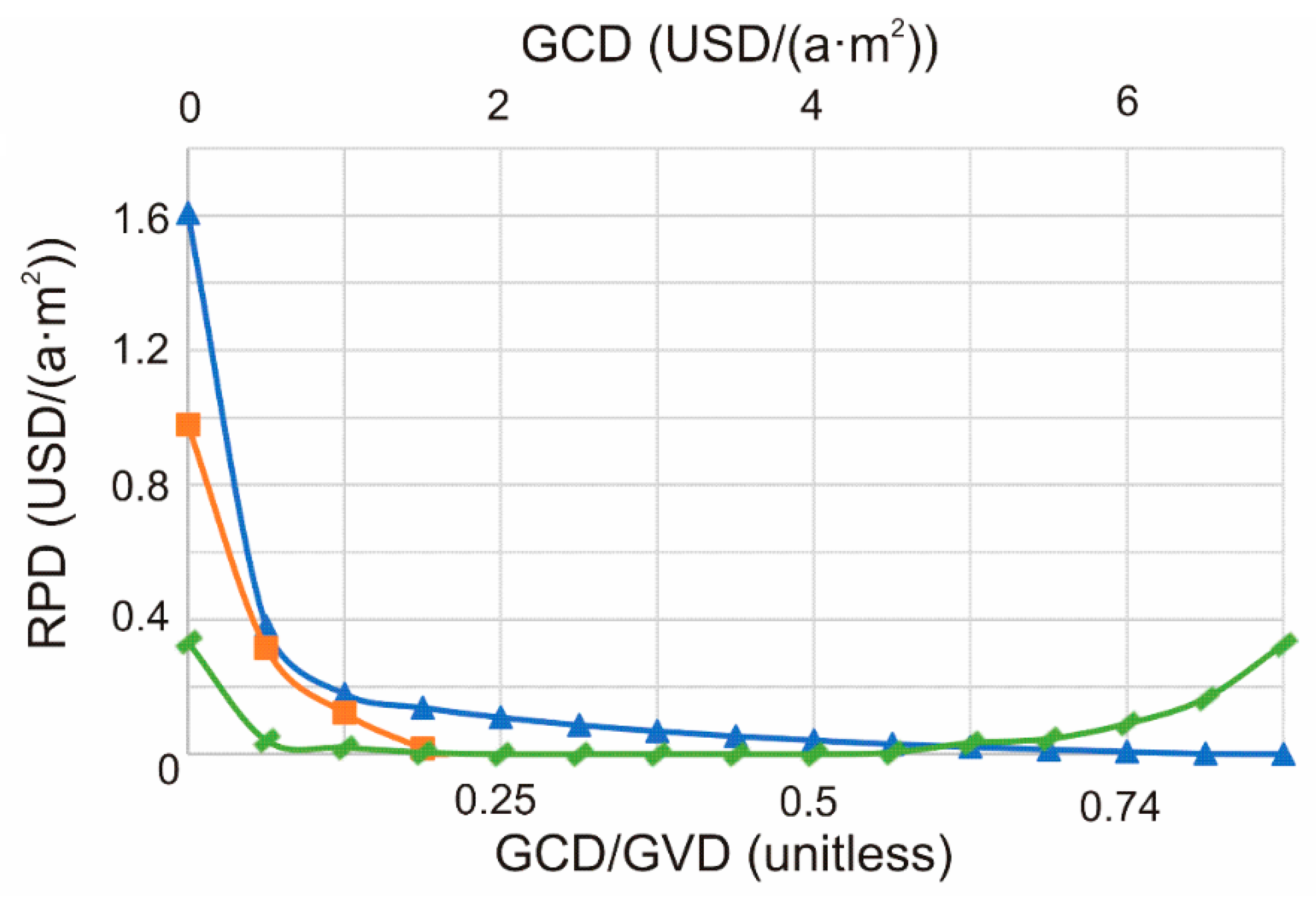
3.3. Economic Analyses (of Generated Value versus Incurred Cost)

The economic analyses of the solar arrays consider their generated value of electricity versus their incurred cost under conditions of high solar penetration. The focus of the study was Bakersfield, California (35° N, 119° W) given its proximity to several hotspots for solar power generation and its vicinity to Los Angeles, where there is a high density of solar rooftop installations. The locale was studied from 2013 to 2018 with temperature data drawn from the National Oceanic and Atmospheric Administration (NOAA) Online Weather Data Service [53] and electricity price data consisting of day-ahead marginal prices from CAISO’s Open-Access Same-Time Information System (OASIS) [3]. Data were collected at 1-h intervals over the 5-year study with negative prices treated as zero. Such zeroing assumed that the solar generation would be disconnected during times of negative electricity prices, which is a fair assumption. The study proceeds as follows:

• Specular and diffuse solar irradiance is computed via Equations (3) and (4), respectively;
• The captured optical power density is then computed for each of the flat-panel, angled-panel, V-groove, and U-groove arrays via Equations (7), (18), (29) and (51), respectively;
• The generated electrical power is then computed for each array using its captured optical power density, the NOAA temperature data from [53], and the I–V characteristics of Equation (1), assuming that each array has one maximum power point tracking (MPPT) system;
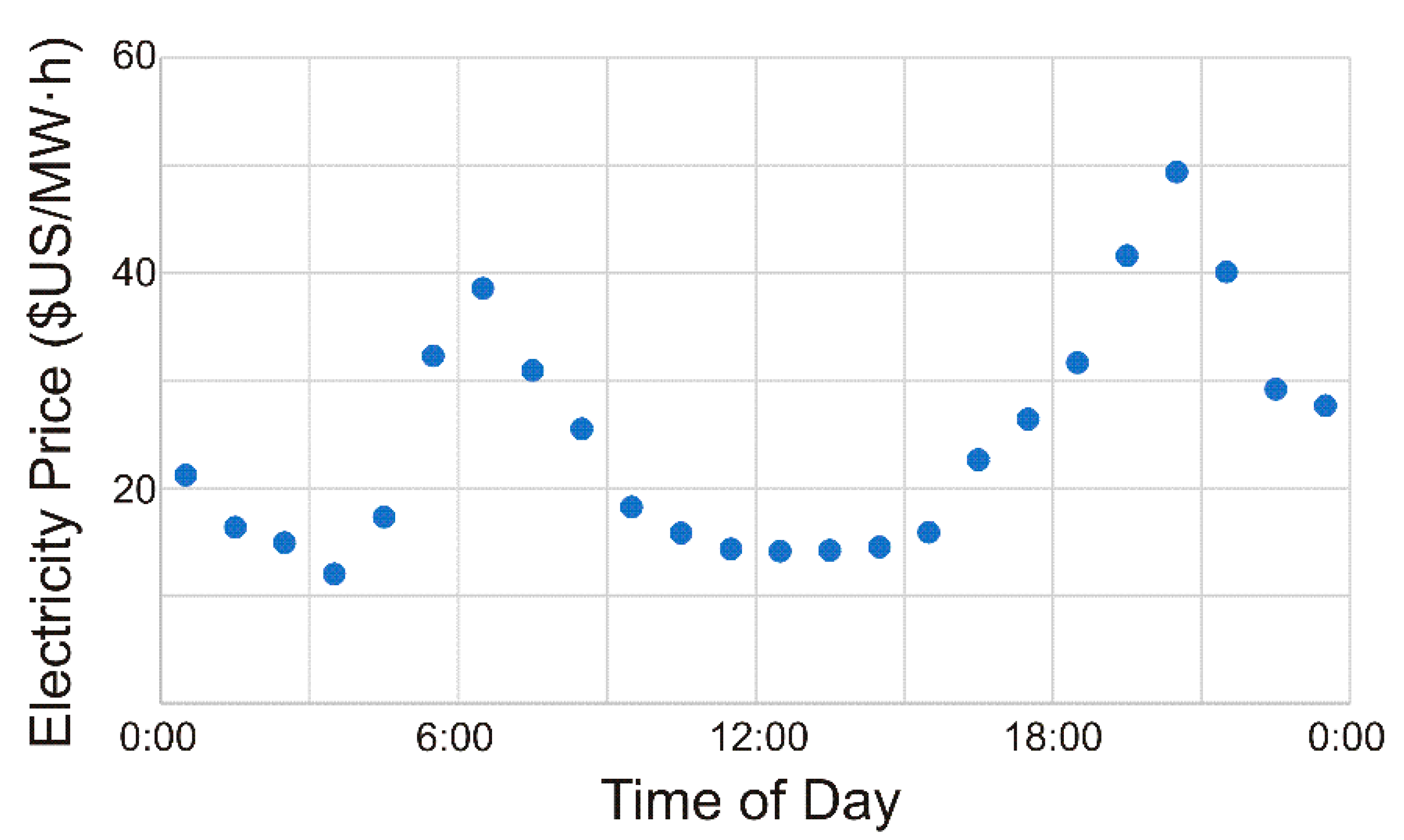
• The generated value of electricity is then computed for each array as an accumulating product of generated electrical power and CAISO OASIS electricity pricing data from [3].

The solar arrays are compared in this work by a metric that we will refer to as the relative profit density (RPD). The term profit is applied here because this metric quantifies the accumulated value of electricity generated by a solar array less its costs in United States Dollars (USD). The terms relative and density signify that the results for a given solar array are normalized with respect to those of the flat-panel array and quoted per annum and unit area. The area here refers to the solar array’s installation area, spanning the horizontal plane. For all but the flat-panel array, this area differs from the solar array’s surface area, which spans the three-dimensional surface of the actual solar cells. The metric of RPD introduced here is similar to prior economic analyses of solar arrays [54], and parallels the metric used by Awad et al. [55], although this study encompasses time-varying electricity prices in its characterization of accumulated values and costs.

The RPD of a given solar array is derived from its total profit, which is the difference between its total generated value and incurred cost over its lifespan. Thus, the total profit can be expressed as v_GLA − (c_f + c_aA + c_sC_GA), where the subscript G identifies the solar array geometry as flat-panel (FP), angled-panel (AP), V-groove (VG), or U-groove (UG). The total generated value is stated here as a product of the solar array’s generated value of electricity per annum and unit area, v_G, lifespan, L, and installation area, A. The total cost is denoted by the terms in parentheses. The first term is the fixed cost, c_f, which incorporates all costs that are roughly independent of the solar array size. In practice, most costs scale with array size to an extent, but costs such as permits and grid interconnection have little dependence on the array size. The second term, c_aA, includes an installation-area-dependent multiplier of c_a for costs that scale in proportion to the installation area, A, such as land cost. Note that the RPD in our work is relative, making the results independent of this (and the first) term. Thus, relative comparisons and generalized conclusions can be obtained without worry over these common costs, which often vary with the locale. The third term, c_sC_GA, scales in proportion to a constant surface-area-dependent multiplier, c_s, and the PV surface area, C_GA. A representative value of c_s = 175 USD/m² is used in our work, as discussed below, whereas the geometry-dependent cost factor, C_G, is calculated as the ratio of PV surface area to installation area. This gives C_G = 1, d_AP/s_AP, 2d_VG/s_VG, and (2h_UG + s_UG)/s_UG for the flat-panel, angled-panel, V-groove, and U-groove arrays, respectively. Ultimately, this third term shows us that arrays with higher vertical-to-horizontal aspect ratios, or more closely spaced/overlapping PV modules, will have these costs scale at an increased rate with respect to the installation area.

Given the above definitions, the RPD of a solar array can be defined as the difference between its total profit and that of the flat-panel array, normalized with respect to the lifespan, L, and installation area, A. Such differencing eliminates the common terms containing c_f and c_a. The RPD_G for the solar array geometry G can then be manipulated into

$${\mathrm{RPD}}_{\mathrm{G}}=\mathrm{GVD}(\hspace{0.17em}{V}_{\mathrm{G}}-1\hspace{0.17em})-\mathrm{GCD}(\hspace{0.17em}{C}_{\mathrm{G}}-1\hspace{0.17em}).$$

(52)

Here, the first term characterizes the solar array’s generated value of electricity per annum and unit area with respect to that of the flat-panel array. It includes a geometric value density (GVD) that is equivalent to the flat-panel array’s generated value of electricity per annum and unit area, i.e., v_FP, and a geometry-dependent value factor, V_G, that is the ratio of the value generated by the given solar array to that of the flat-panel array. Thus, V_G quantifies the extent to which a given solar array generates value over that of the flat-panel array with the GVD acting as an external scaling factor for this value. The second term characterizes the solar array’s surface-area-dependent costs per annum and unit area with respect to those of the flat-panel array. It includes a geometric cost density (GCD), which is equivalent to the surface-area-dependent multiplier divided by the lifespan, i.e., c_s/L, and a geometry-dependent cost factor, C_G. Thus, C_G quantifies the cost of a solar array over that of a flat-panel array with the GCD as an external scaling factor for this cost.

Clearly, the profit captured by a given solar array, as defined by the RPD, can be optimized by maximizing the value factor, V_G, and minimizing the cost factor, C_G. However, this must be done while recognizing that the GVD and GCD magnify the effects of value and cost while being set by prevailing supply-and-demand economics. The GVD is linked to cycles of supply and demand in electricity prices, such that it scales with midday electricity prices. Thus, economies having strong Duck Curve characteristics with reduced electricity prices at midday exhibit low GVD. This can be understood by recalling that the GVD quantifies the flat-panel array’s generated value of electricity per annum and unit area as a nominal value with the greatest sensitivity to diurnal fluctuations in electricity prices. (The other solar arrays have geometries that can better trap light at early- and late-day hours, which increases their value factor, V_G, and offers them some protection from diurnal fluctuations in electricity prices). The GCD is linked to supply and demand in costs of solar infrastructure. Thus, improvements and overall growth in the manufacture of PV modules over the past decade [56] has led to a steady decrease in the GCD. Based on the data of Fu et al. [56], such costs are approximately 7 USD/(a·m²) at present for a solar efficiency of 17% [57], such that a 1 m² solar module with a lifespan of 25 years would have an estimated cost (and thus surface-area-dependent multiplier) of c_s = 175 USD/m². The decline in GCD suggests that solar arrays with heightened aspect ratios and greater values of C_G may now outperform the industry-standard angled-panel array from the standpoint of value. Such a prospect is explored and discussed in the following section.

4. Results and Discussions

Results for the optimization and contrasting of the proposed solar arrays are shown in this section, with an overarching discussion on historical and future trends.

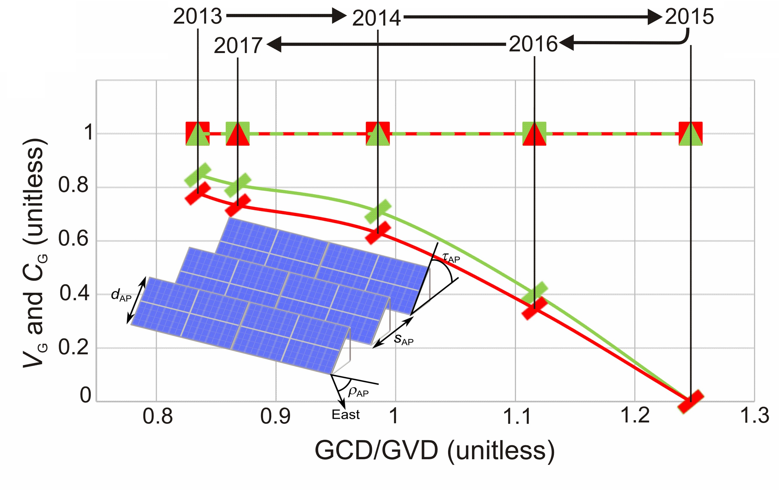
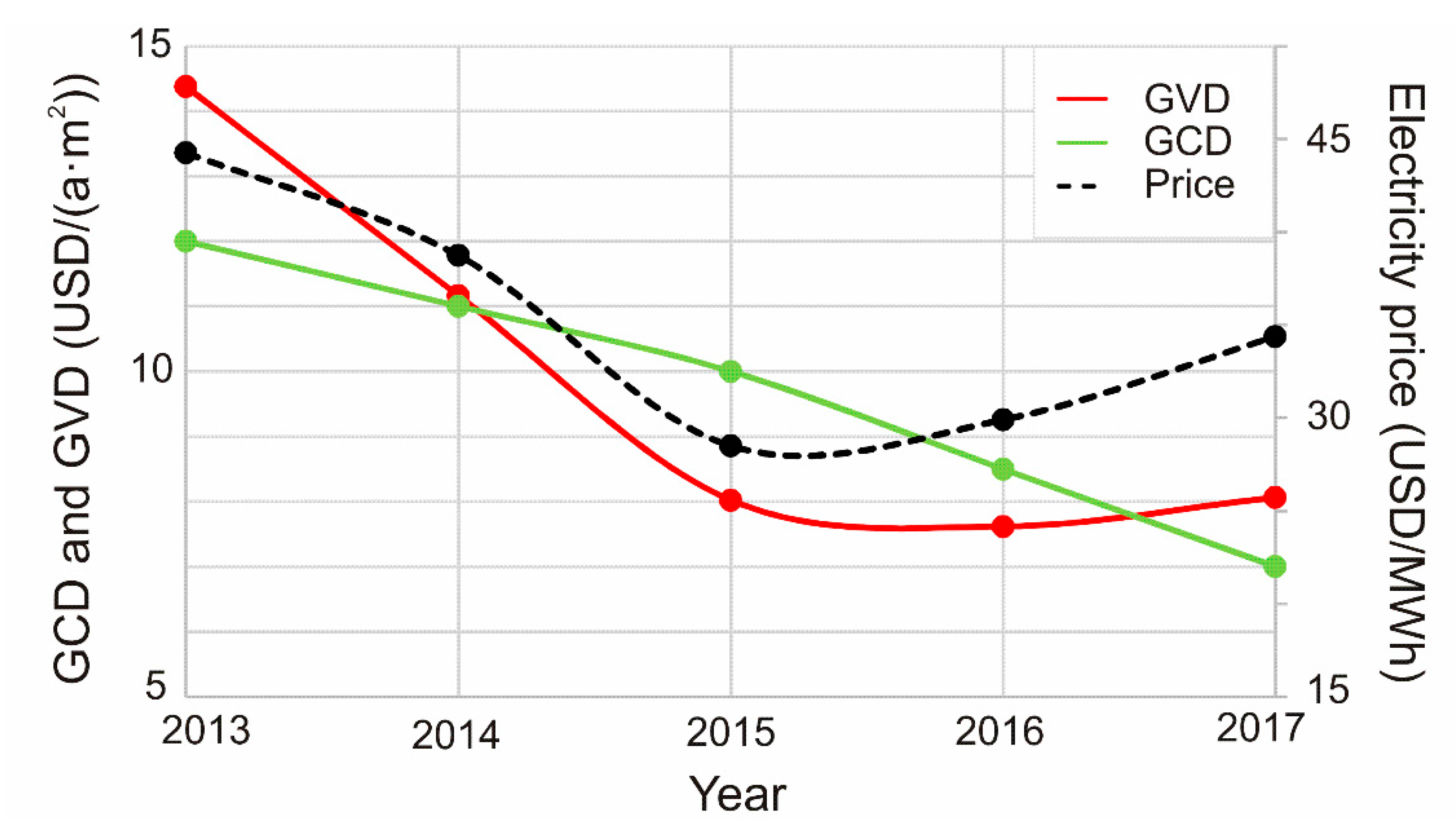
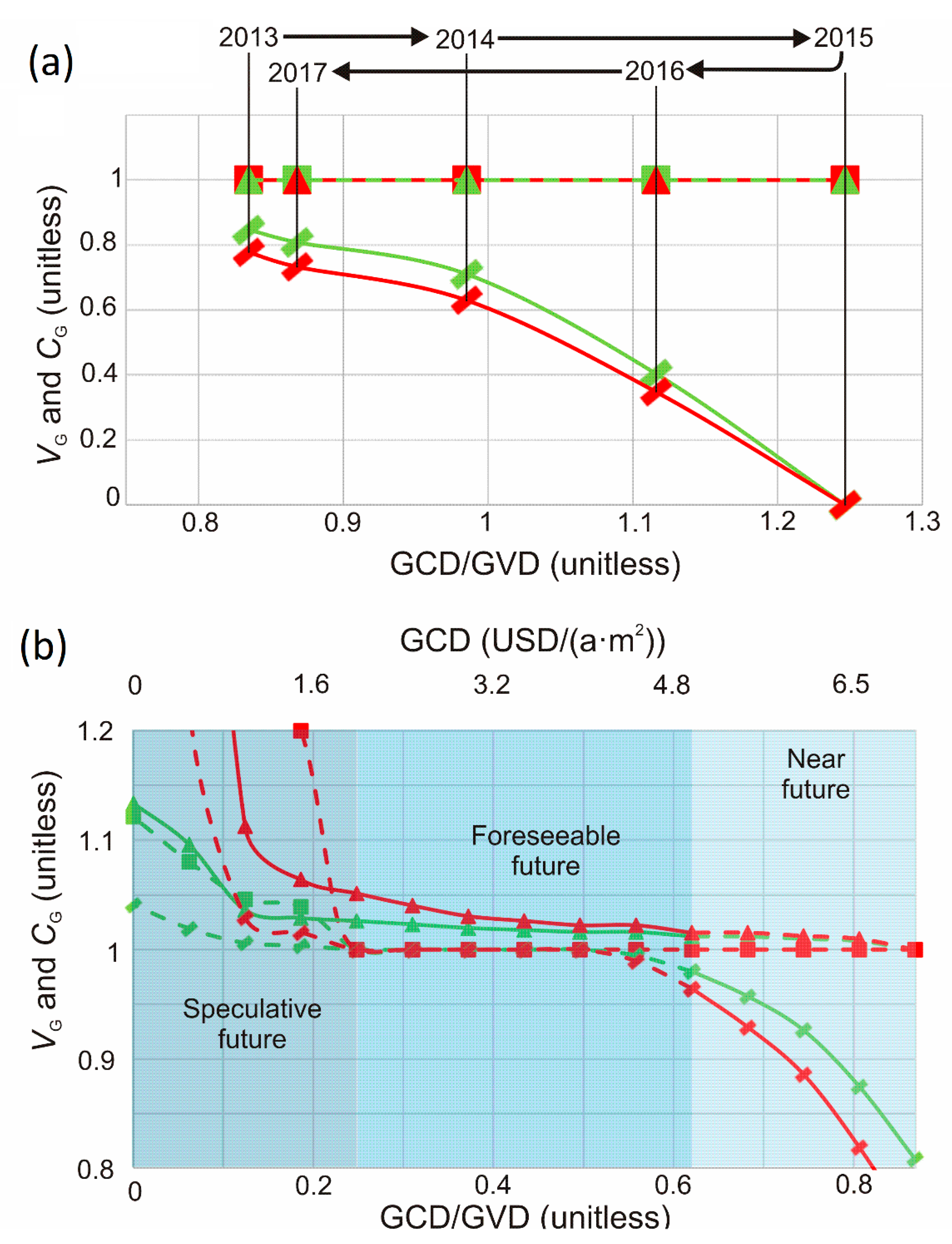
4.1. Historical Trends

The performance levels of the proposed solar arrays are linked to market conditions by way of the GVD and GCD, which are shown in Figure 3 for a 5-year history at the stated location in California (35° N, 119° W). The history starts on 1 July, 2013, and ends on 30 June, 2018, with each year spanning 1 July to 30 June. Thus, the five years of this study span 2013-14, 2014-15, 2015-16, 2016-17, and 2017-18.

The GVD, displayed as a solid red curve in Figure 3 against the left axis, is calculated from the flat-panel array’s value per annum and unit area given the average electricity price, displayed as a dotted black curve against the right axis. Here, the earlier 3 years exhibit roughly linear correlation between GVD and average electricity price, leading to overlapping curves, while the latter 2 years show divergence in the curves. Such trends can be understood by noting that the GVD is sensitive to diurnal cycles in electricity price, given that generated electrical power is greatest during midday hours and least during early- and late-day hours, while the average electricity price, as a mean over the day, is far less sensitive to these diurnal cycles. Thus, strengthening Duck Curve characteristics, with midday prices reducing below early- and late-day prices, preferentially reduce the GVD, decreasing the ratio between it and the average electricity price. This is seen in the latter 2 years, whereby the GVD remains roughly constant despite an increasing average electricity price. Over a longer term, we would see such Duck Curve characteristics manifest as a generalized reduction in the GVD.

The GCD, displayed as a solid green curve in Figure 3 against the left axis, is calculated by scaling the present-day infrastructure costs, which give the aforementioned 7 USD/(a·m²), over historical trends [56]. The evolving GCD is in contrast to the GVD, in that it shows a simple monotonic decrease over the displayed 5-year history.

Given the stated reductions in GVD, due to intensifying Duck Curve characteristics, and GCD, due to decreasing infrastructure costs, the goal to maximize profit can be cast as a competition between value and cost. The competition manifests via Equation (52), with the GVD and GCD magnifying effects of the value factor, V_G, and cost factor, C_G. The results show GVD decreasing at a slower rate than GCD, which has the first term dominate with V_G taking on greater importance than C_G. This suggests that the increased costs of complex solar arrays, from greater vertical-to-horizontal aspect ratios, are offset (to an extent) by their increased value generation under Duck Curve characteristics.

Given that each solar array’s value and cost are a function of its geometric parameters, as displayed in Figure 2 and defined in Section 2, the overall profit of each array must be computed and (ideally) maximized. Thus, the generated value is computed for each solar array, using the analyses of Section 3 for all combinations of parameters over the 5-year study. The parameters that yield a maximal value factor, V_G, and minimal cost factor, C_G, then give the greatest profit and maximal RPD. The V_G and C_G for the fully optimized angled-panel, V-groove, and U-groove arrays are shown in Figure 4, with Figure 4a showing the results over a 5-year history plotted against the GCD-to-GVD ratio. The (horizontal) unity line in this subfigure characterizes the flat-panel array. Thus, the separation of V_G and C_G from the unity line portrays the degree to which an optimal structure deviates from a flat-panel array. With this interpretation, we see the V-groove and U-groove arrays degenerate into the flat-panel array via their optimization, with optimal geometric parameters of ν_VG = 180° and s_UG = ∞, respectively, yielding unity V_G and C_G. This trend can be explained by noting that C_G can only be at or above unity for these arrays, and historical values of GCD have been high enough to have the optimization primarily minimize C_G. The trends exhibited by V_AP and C_AP are in contrast to this. They are far below unity, showing that the optimal angled-panel array deviates greatly from the flat-panel array. Thus, the reduced V_AP is deemed to be acceptable (and even optimal) given the associated reduction in C_AP. As the GCD-to-GVD ratio increases along the horizontal axis, the RPD optimization preferentially drives the C_AP down in spite of further reductions in V_AP, causing the optimal angled-panel array to deviate further from the flat-panel array. (An excessively high GCD causes both C_AP and V_AP to drop to zero, characterizing conditions antithetical to solar power generation, whereby a degenerate case of no solar cells is optimal). Conversely, as the GCD-to-GVD ratio decreases, the RPD optimization places greater importance on a heightened V_AP, causing the optimal angled-panel array to approach a flat-panel array. Such trends, of the angled-panel array approaching the flat-panel array and higher C_G values becoming acceptable, suggest that further decreases in GCD could make the angled-panel array non-viable and the V-groove and U-groove arrays viable.

The optimal geometric parameters for the angled-panel array for each of the previous 5 years are tabulated in

Table 1. Optimized values of geometric parameters for the angled-panel array for each year.

Year	sAP (mm)	τAP (°)	ρAP (°)
2013–2014	98	18	−5
2014–2015	121	27	−10
2015–2016	∞	41	−20
2016–2017	219	37	−20
2017–2018	104	21	−15

. The data shows that the lower values of V_AP and C_AP seen in Figure 4a correspond to larger spacings, s_AP, reducing the array density and thereby both geometry-dependent factors, as well as higher tilt angles, τ_AP, which increase as array self-shadowing decreases. For this value-based optimization, such angles ultimately reach 6° more than the latitude, which is slightly more than the tilt angles generally considered optimal for standalone PV modules under power-based optimization [58]. The rotation angle, ρ_AP, meanwhile, does not closely follow the geometry-dependent factors, but rather generally decreases with time, leading the array to point further west over time. This trend demonstrates the direct relation between the optimal values of ρ_AP and the severity of the Duck Curve characteristics, which has the west-facing solar cells preferentially capture light during the late-day hours when electricity prices are the highest.

Overall, given the general trend of a decreasing GCD-to-GVD ratio, value-based optimization is trending towards solar arrays of greater complexity, with higher values of V_G and C_G. Thus, the heightened values for the V-groove and U-groove arrays, even in spite of their higher costs, may allow them to outperform the angled-panel array in the future—a possibility that warrants the investigation in the following subsection.

4.2. Future Trends

The identification of future value-based trends is important for planning and design of new solar arrays, but such a goal is hampered by uncertainty in electricity prices and infrastructure costs. Nonetheless, it is possible to build a framework for future value-based design and analysis of solar arrays based upon trends in these prices and costs.

The electricity prices and infrastructure costs arising through the GVD and GCD have general trends. The GVD is highly dependent on the price of electricity, which fluctuates greatly over timespans of years, and it is also a relevant metric over the lifespan of an array, which can exceed 30 years [59]. Given these rapid fluctuations over a long span of time, and an assumption that the Duck Curve characteristics remain consistent over this span, the GVD is taken as a constant here. It is fixed at 8.06 USD/(a·m²), as defined earlier from the final year of the 5-year history. The electricity prices are also fixed at those observed during this final year. The GCD, in contrast, is easier to define. It has fallen with a rate of decrease that is slowing and is trending to a plateau. Thus, the GCD is treated as an independent variable in this work, with values spanning from the present 7 USD/(a·m²) down to an extreme of 0 USD/(a·m²), representing zero infrastructure costs.

The optimal RPD for the three arrays as a function of the GCD (and the corresponding GCD-to-GVD ratio) is shown in Figure 5. The optimization is performed for all geometric parameters but each array’s rotation angle, which is fixed at zero. Such a simplification is done to minimize the complexity of the optimization while recognizing from the prior section that the optimal rotation angle has only a weak dependence on the GVD and GCD. (While it is not presented here, it can be shown that optimization of the rotation angle yields significant changes in the RPD only near the lower and upper limits of the GCD in this figure). For the presented figure, the angled-panel array has a significant RPD at current values of the GCD, but the RPD quickly drops to zero as GCD decreases. Conversely, the V-groove array has zero RPD at current values of GCD, but the RPD increases as GCD drops. Thus, there is a point at a GCD of approximately 5 USD/(a·m²) where the two arrays have equivalent RPDs. If the GCD drops through this crossover point, the best-performing solar array will transition from the angled-panel array to the V-groove array. At very low GCD, the RPDs of the angled-panel and U-groove arrays increase, but neither array experiences enough performance improvement to surpass the V-groove array.

Figure 4b shows predictions for the value factor, V_G, and cost factor, C_G, in the future as a function of the GCD (and the corresponding GCD-to-GVD ratio). Given the decreasing GCD over the years, the right side of this subfigure can be interpreted as the present, and progression to the left on this subfigure can be cast as trends into the future. The trends are discussed here in ranges of GCD-to-GVD ratios corresponding to the near, foreseeable, and speculative future. (These ratios are based upon realistic parameters, and thus give reliable predictions of trends, but labels of near, foreseeable, and speculative are used here for timespans in the future, rather than precise years, because uncertainties in solar energy markets can affect the years in which such trends emerge.) The optimal geometric parameters for each array across these ranges are tabulated in

Table 2. Optimized values of geometric parameters for each array and each geometric cost density. Rotation angles are fixed at zero for optimization. For U-groove arrays at high geometry-dependent cost density values, precise optimization is not possible, as the arrays become arbitrarily large.

GCD (USD/(a·m2))	GCD/GVD	sAP (mm)	τAP (°)	νVG (°)	sUG (mm)
0	0	30	34	31	76.2
0.5	0.062	62	9	68	228.6
1	0.124	74	1	128	609.6
1.5	0.186	75	1	140	≥762
2	0.248	76.2	0	144	>7620
2.5	0.31	76.2	0	148	>7620
3	0.372	76.2	0	152	>7620
3.5	0.434	76.2	0	154	>7620
4	0.496	76.2	0	156	>7620
4.5	0.558	77	2	156	>7620
5	0.62	79	5	160	>7620
5.5	0.682	82	8	160	>7620
6	0.744	86	11	162	>7620
6.5	0.806	93	15	164	>7620
7	0.868	103	19	180	>7620

.

In the near future, moderately reduced silicon solar cell costs will lead to GCD-to-GVD ratios of 0.87 down to 0.62. In this range, the trend seen for the angled-panel array in Figure 4a continues, with V_AP and C_AP both approaching unity as the GCD decreases. This has the optimal angled-panel array approach the flat-panel array. Over this range, the optimal V-groove array has V_VG and C_VG slightly above unity, representing a small deviation from the flat-panel array, while the optimal U-groove array remains degenerate. These results are reflected in Figure 5, whereby the angled-panel array has a large positive RPD, the V-groove array has a small positive RPD, and the U-groove array has zero RPD over this range. Moreover, the optimal geometric parameters (tabulated in Table 2) show that the optimal V-groove array has a large ν_VG near 180°, and the optimal angled-panel array has initially large s_AP and τ_AP, which decrease towards 76.2 mm and 0°, respectively, as the GCD decreases. Such trends agree with predictions of Awad et al. [55]. Overall, the findings suggest the angled-panel array will continue to show the best performance in the near future, but its relative performance will lessen as the GCD decreases.

In the foreseeable future, significantly reduced silicon solar cell costs will lead the GCD-to-GVD ratio of 0.62 down to 0.25. In this range, Figure 4b shows all three arrays with V_G and C_G close to unity, suggesting the optimal arrays are all similar to a flat-panel array. The U-groove array remains degenerate across the entirety of this range. Following previously seen trends, the angled-panel array also becomes degenerate and remains that way across the majority of this range. Both of these are reflected in the zero RPD seen in Figure 5 and the degenerate parameters seen in Table 2. By contrast, while V_VG and C_VG remain close to unity, the V-groove array is not degenerate, but continues to display small positive values for the RPD and large ν_VG near but not equal to 180° over the entirety of this range. Ultimately, it can be said that the V-groove array will show the best performance over the foreseeable future—with stable performance in this range. None of the optimized parameters vary significantly with changing GCD-to-GVD ratios, which suggests that significant swings in the GVD caused by volatile electricity prices would not disrupt the performance of the V-groove array under these conditions.

In the speculative future, negligible silicon solar cell costs may lead to GCD-to-GVD ratios of 0.25 down to 0. In this range, Figure 4b shows V_G and C_G for all three arrays rising significantly above unity, with the increase in C_G being more dramatic than that of V_G. This suggests that increasing C_G above unity yields diminishing returns in increased V_G, which can only be justified if the GCD is very low, making costs unimportant. This scenario will only occur if the cost of silicon solar cells drops dramatically. Figure 5 shows that while the RPDs of all three arrays increase significantly in this range, the V-groove array remains the top-performing array over the full range. The optimal geometric parameters (tabulated in Table 2) show that the increased values and costs of all three arrays can be linked to high vertical-to-horizontal aspect ratios with the key geometric parameters of s_AP, ν_VG, and s_UG all decreasing significantly over this range. These more complex structures have significantly higher costs per unit area, but they yield improved light capture.

It is worth emphasizing that the above results are potential outcomes for economic conditions that are subject to uncertainty. First, while the decrease in the GCD is well-established, the rate at which this decrease occurs as well as where it will ultimately stabilize cannot be known with certainty. Second, the significant variations in the GVD are not easily characterized and may disguise additional long-term trends, while the observed trend due to the Duck Curve is contingent on future worsening or lessening of that phenomenon. Third, each array’s V_G depends upon hourly electricity prices in a manner that is not fully encompassed by the GVD, and the marginal electricity prices used in calculating the V_G and GVD do not fully represent the rates at which electricity is purchased from solar generation systems. Such rates are typically higher and less variable due to power purchase agreements and renewable energy subsidies [60]. Nonetheless, the core conclusions of this work are sound: The trends seen for the supply and demand of solar-generated power and solar cell prices will lead to shallow-angled V-groove arrays outperforming industry-standard angled-panel arrays, in terms of profit, with such arrays having reduced sensitivity to electricity price fluctuations.

Future studies may expand upon this work with added complexity. For example, tracking and non-tracking solar arrays could be analysed in terms of generated value of electricity versus incurred costs. However, such analyses must note that tracking systems have far higher infrastructure costs and the greatest benefits at large row separations (with reduced shadowing) [23]. Moreover, tracking solar arrays yield disproportionately high generated power from their unshadowed perimeters, and so the analyses could no longer be performed normalized with respect to (and thus independent of) the installation area. As a second example, off-ground distances of the solar arrays could be considered. This distance can impact the solar arrays’ costs, as higher off-ground distances demand larger support structures, as well as the solar arrays’ convective cooling, with higher off-ground distances yielding greater efficiency, as seen in [26,27,28,29,30]. Such cooling could be analysed by lessening the power-dependent self-heating, which was fixed in this work. This would decrease the saturation currents and series resistances and increase the efficiency. Lastly, the off-ground distance could be optimized for use with bifacial PV modules to maximize the capture of optical power from the surroundings [61].

5. Conclusions

This work considered an emerging value-based paradigm for solar power generation. Such a paradigm can manifest in conditions of high solar penetration due to conflicting cycles of supply and demand for electricity over the day. This yields dramatic swings in the price of electricity, as characterized by the Duck Curve in locales such as California, which calls into question the conventional aim of optimizing solar arrays solely in terms of their electrical power. Instead, it becomes necessary to consider the value as an accumulated product of electrical power and price. To this end, solar arrays that generate electrical power over a broader duration of time, spanning the low-supply and high-demand hours with higher electricity prices, would yield greater value and be more desirable.

In light of these emerging conditions, the presented work looked at the value-based performance of angled-panel, V-groove, and U-groove arrays. Experimental analyses were put forward to define characteristics for the constituent silicon solar cells, which can exhibit time-varying functionality and nonideality in realistic/field conditions, while theoretical analyses were applied to quantify each array’s ability to capture incident optical power. This was done with consideration for all manners of solar illumination, including specular (direct) and diffuse (indirect) incidence as well as the ensuing specular (mirror-like) and diffuse (scattered) reflections within the arrays. The experimental and theoretical analyses were then integrated within economic analyses using electrical price data and infrastructure costs. A 5-year history was tracked for a locale with high solar penetration to identify and contrast the optimal configurations of the arrays. The historical results showed that the optimal solar arrays are trending towards greater complexity, as higher vertical-to-horizontal aspect ratios, given the improved light-capturing abilities of these complex arrays over the early- and late-day hours and the decreasing infrastructure costs of the constituent solar cells. The analyses were then projected into the near, foreseeable, and speculative future. Findings for the near future showed that the angled-panel array will continue to exhibit the best performance, although its relative performance will decrease as infrastructure costs continue to decrease. Findings for the foreseeable future suggested that the V-groove array will begin to outperform the other arrays, with a level of performance that is relatively insensitive to electricity prices. Such stable operation is advantageous given the volatility that is seen in electricity prices. Findings for the speculative future suggested that all of the arrays will trend towards complex forms, with high vertical-to-horizontal aspect ratios, although the V-groove array will continue to yield the best performance. Ultimately, it is hoped that the insight put forward here will foster the continued study (and growth) of solar technology.

References

1. International Energy Agency (IEA). Photovoltaic Power System Programme (PVPS). In 2016 Snapshot of Global Photovoltaic Markets; IEA: Paris, France, 2016. [Google Scholar]
2. California Independent System Operator (CAISO). Demand Response and Energy Efficiency Roadmap: Maximizing Preferred Resources; CAISO: Folsom, California, 2013. [Google Scholar]
3. California Independent Systems Operator (CAISO) Open-Access Same-Time Information System (OASIS) website. Available online: https://oasis.caiso.com (accessed on 15 September 2018).
4. Li, M.; Pan, J.; Su, Q.; Niu, Y. Analyzing sensitivity of power system wind penetration to thermal generation flexibility. In Proceedings of the 2017 13th IEEE Conference on Automation Science and Engineering (CASE), Xi’an, China, 20–23 August 2017; pp. 1628–1632. [Google Scholar]
5. Obi, M.; Bass, R. Trends and challenges of grid-connected photovoltaic systems–A review. Renew. Sustain. Energy Rev. 2016, 58, 1082–1094. [Google Scholar] [CrossRef]
6. Janko, S.A.; Arnold, M.R.; Johnson, N.G. Implications of high-penetration renewables for ratepayers and utilities in the residential solar photovoltaic (PV) market. Appl. Energy 2016, 180, 37–51. [Google Scholar] [CrossRef]
7. Hassan, A.S.; Cipcigan, L.; Jenkins, N. Optimal battery storage operation for PV systems with tariff incentives. Appl. Energy 2017, 203, 422–441. [Google Scholar] [CrossRef]
8. Schoenung, S.M.; Keller, J.O. Commercial potential for renewable hydrogen in California. Int. J. Hydrog. Energy 2017, 42, 13321–13328. [Google Scholar] [CrossRef]
9. Zhang, N.; Lu, X.; McElroy, M.B.; Nielsen, C.P.; Chen, X.; Deng, Y.; Kang, C. Reducing curtailment of wind electricity in China by employing electric boilers for heat and pumped hydro for energy storage. Appl. Energy 2016, 184, 987–994. [Google Scholar] [CrossRef] [Green Version]
10. Gür, T.M. Review of electrical energy storage technologies, materials and systems: Challenges and prospects for large-scale grid storage. Energy Environ. Sci. 2018, 11, 2696–2767. [Google Scholar] [CrossRef]
11. Chaudhary, P.; Rizwan, M. Energy management supporting high penetration of solar photovoltaic generation for smart grid using solar forecasts and pumped hydro storage system. Renew. Energy 2018, 118, 928–946. [Google Scholar] [CrossRef]
12. Le Floch, C.; Belletti, F.; Moura, S. Optimal Charging of Electric Vehicles for Load Shaping: A Dual-Splitting Framework With Explicit Convergence Bounds. IEEE Trans. Transp. Electrif. 2016, 2, 190–199. [Google Scholar] [CrossRef]
13. Sanandaji, B.M.; Vincent, T.L.; Poolla, K. Ramping Rate Flexibility of Residential HVAC Loads. IEEE Trans. Sustain. Energy 2015, 7, 865–874. [Google Scholar] [CrossRef]
14. Perez, M.; Perez, R.; Rábago, K.R.; Putnam, M. Overbuilding & curtailment: The cost-effective enablers of firm PV generation. Sol. Energy 2019, 180, 412–422. [Google Scholar] [CrossRef]
15. Perez, R.; Perez, M.; Schlemmer, J.; Dise, J.; Hoff, T.E.; Swierc, A.; Keelin, P.; Pierro, M.; Cornaro, C. From Firm Solar Power Forecasts to Firm Solar Power Generation an Effective Path to Ultra-High Renewable Penetration a New York Case Study. Energies 2020, 13, 4489. [Google Scholar] [CrossRef]
16. Perez, R.; Rábago, K.R.; Trahan, M.; Rawlings, L.; Norris, B.; Hoff, T.; Putnam, M.; Perez, M. Achieving very high PV penetration–The need for an effective electricity remuneration framework and a central role for grid operators. Energy Policy 2016, 96, 27–35. [Google Scholar] [CrossRef] [Green Version]
17. Borenstein, S. The Market Value and Cost of Solar Photovoltaic Energy Production; Center for the Study of Energy Markets: Berkeley, CA, USA, 2008. [Google Scholar]
18. Hartner, M.; Ortner, A.; Hiesl, A.; Haas, R. East to west–The optimal tilt angle and orientation of photovoltaic panels from an electricity system perspective. Appl. Energy 2015, 160, 94–107. [Google Scholar] [CrossRef]
19. Rowlands, I.H.; Kemery, B.P.; Beausoleil-Morrison, I. Optimal solar-PV tilt angle and azimuth: An Ontario (Canada) case-study. Energy Policy 2011, 39, 1397–1409. [Google Scholar] [CrossRef]
20. Masrur, H.; Konneh, K.; Ahmadi, M.; Khan, K.; Othman, M.; Senjyu, T. Assessing the Techno-Economic Impact of Derating Factors on Optimally Tilted Grid-Tied Photovoltaic Systems. Energies 2021, 14, 1044. [Google Scholar] [CrossRef]
21. Maleki, S.A.M.; Hizam, H.; Gomes, C. Estimation of Hourly, Daily and Monthly Global Solar Radiation on Inclined Surfaces: Models Re-Visited. Energies 2017, 10, 134. [Google Scholar] [CrossRef] [Green Version]
22. Al-Rousan, N.; Isa, N.A.M.; Desa, M.K.M. Advances in solar photovoltaic tracking systems: A review. Renew. Sustain. Energy Rev. 2018, 82, 2548–2569. [Google Scholar] [CrossRef]
23. Vasantha, P.N.; Dehankar, S.; Raman, M.; Karnataki, K.; Shankar, G. Space optimization and backtracking for dual axis so-lar photovoltaic tracker. In Proceedings of the IEEE International WIE Conference on Electrical and Computer Engineering, Dhaka, Bangladesh, 19–20 December 2015; pp. 451–454. [Google Scholar]
24. Brecl, K.; Topic, M. Self-shading losses of fixed free-standing PV arrays. Renew. Energy 2011, 36, 3211–3216. [Google Scholar] [CrossRef]
25. Gordon, J.; Wenger, H.J. Central-station solar photovoltaic systems: Field layout, tracker, and array geometry sensitivity studies. Sol. Energy 1991, 46, 211–217. [Google Scholar] [CrossRef]
26. Vaillon, R.; Dupré, O.; Cal, R.B.; Calaf, M. Pathways for mitigating thermal losses in solar photovoltaics. Sci. Rep. 2018, 8, 13163. [Google Scholar] [CrossRef]
27. Stanislawski, B.; Margairaz, F.; Cal, R.; Calaf, M. Potential of module arrangements to enhance convective cooling in solar photovoltaic arrays. Renew. Energy 2020, 157, 851–858. [Google Scholar] [CrossRef]
28. Glick, A.; Smith, S.E.; Ali, N.; Bossuyt, J.; Recktenwald, G.; Calaf, M.; Cal, R.B. Influence of flow direction and turbulence intensity on heat transfer of utility-scale photovoltaic solar farms. Sol. Energy 2020, 207, 173–182. [Google Scholar] [CrossRef]
29. Glick, A.; Ali, N.; Bossuyt, J.; Calaf, M.; Cal, R.B. Utility-scale solar PV performance enhancements through system-level modifications. Sci. Rep. 2020, 10, 1–9. [Google Scholar] [CrossRef] [PubMed]
30. Glick, A.; Ali, N.; Bossuyt, J.; Recktenwald, G.; Calaf, M.; Cal, R.B. Infinite photovoltaic solar arrays: Considering flux of momentum and heat transfer. Renew. Energy 2020, 156, 791–803. [Google Scholar] [CrossRef]
31. Sista, S.; Hong, Z.; Chen, L.-M.; Yang, Y. Tandem polymer photovoltaic cells—current status, challenges and future outlook. Energy Environ. Sci. 2011, 4, 1606–1620. [Google Scholar] [CrossRef]
32. Andersson, B.V.; Würfel, U.; Inganäs, O. Full day modelling of V-shaped organic solar cell. Sol. Energy 2011, 85, 1257–1263. [Google Scholar] [CrossRef]
33. Ding, K.; Zhang, J.; Bian, X.; Xu, J. A simplified model for photovoltaic modules based on improved translation equations. Sol. Energy 2014, 101, 40–52. [Google Scholar] [CrossRef]
34. Humada, A.M.; Hojabri, M.; Mekhilef, S.; Hamada, H.M. Solar cell parameters extraction based on single and double-diode models: A review. Renew. Sustain. Energy Rev. 2016, 56, 494–509. [Google Scholar] [CrossRef] [Green Version]
35. Aberle, A.G.; Zhang, W.; Hoex, B. Advanced loss analysis method for silicon wafer solar cells. Energy Procedia 2011, 8, 244–249. [Google Scholar] [CrossRef] [Green Version]
36. Du, Y.; Tao, W.; Liu, Y.; Le, Z.; Zhang, M. Cell-to-Module Variation of Optical and Photovoltaic Properties for Monocrystalline Silicon Solar Cells with Different Texturing Approaches. ECS J. Solid State Sci. Technol. 2017, 6, P332–P338. [Google Scholar] [CrossRef]
37. Saynova, D.; Mihailetchi, V.; Geerligs, L.; Weeber, A. Comparison of high efficiency solar cells on large area n-type and p-type silicon wafers with screen-printed Aluminum-alloyed rear junction. In Proceedings of the 2008 33rd IEEE Photovolatic Specialists Conference, San Diego, CA, USA, 11–16 May 2008; pp. 1–5. [Google Scholar]
38. Solanki, C.S.; Singh, H.K. Anti-Reflection and Light Trapping in c-Si Solar Cells; Springer Nature: Singapore, 2017. [Google Scholar]
39. Riordan, C.; Hulstron, R. What is an air mass 1.5 spectrum? (solar cell performance calculations). In Proceedings of the IEEE Conference on Photovoltaic Specialists, Kissimmee, FL, USA, 21–25 May 1990; pp. 1085–1088. [Google Scholar]
40. Breitenstein, O. Understanding the current-voltage characteristics of industrial crystalline silicon solar cells by considering inhomogeneous current distributions. Opto-Electron. Rev. 2013, 21, 259–282. [Google Scholar] [CrossRef]
41. Koehl, M.; Heck, M.; Wiesmeier, S.; Wirth, J. Modeling of the nominal operating cell temperature based on outdoor weathering. Sol. Energy Mater. Sol. Cells 2011, 95, 1638–1646. [Google Scholar] [CrossRef]
42. Singh, P.; Ravindra, N. Temperature dependence of solar cell performance—an analysis. Sol. Energy Mater. Sol. Cells 2012, 101, 36–45. [Google Scholar] [CrossRef]
43. Wolf, M.; Noel, G.T.; Stirn, R.J. Investigation of the double exponential in the current-voltage characteristics of silicon solar cells. IEEE T. Electron. Dev. 1977, 24, 419–428. [Google Scholar] [CrossRef]
44. Boivin, A.B.; Westgate, T.M.; Holzman, J.F. Design and performance analyses of solar arrays towards a metric of energy value. Sustain. Energy Fuels 2018, 2, 2090–2099. [Google Scholar] [CrossRef]
45. Boivin, A.B. Performance and value of geometric solar arrays subject to cyclical electricity prices and high solar penetration. Master’s Thesis, The University of British Columbia, Kelowna, BC, Canada, 2019. [Google Scholar]
46. Young, A. Air mass and refraction. Appl. Opt. 1994, 33, 1108–1110. [Google Scholar] [CrossRef]
47. American Society for Testing and Materials (ASTM). G173-03 (2012) Standard Tables for Reference Solar Spectral Irradiances: Direct Normal and Hemispherical on 37° Tilted Surface; American Society for Testing and Materials: West Conshohocken, PA, USA, 2012. [Google Scholar] [CrossRef]
48. American Society for Testing and Materials (ASTM). E490-00a (2014) Standard Solar Constant and Zero Air Mass Solar Spectral Irradiance Tables; American Society for Testing and Materials: West Conshohocken, PA, USA, 2014. [Google Scholar] [CrossRef]
49. Becker, S. Calculation of direct solar and diffuse radiation in Israel. Int. J. Clim. 2001, 21, 1561–1576. [Google Scholar] [CrossRef]
50. Koomen, M.J.; Lock, C.; Packer, D.M.; Scolnik, R.; Tousey, R.; Hulburt, E.O. Measurements of the Brightness of the Twilight Sky. J. Opt. Soc. Am. 1952, 42, 353. [Google Scholar] [CrossRef]
51. Coblentz, W. The diffuse reflecting power of various substances. J. Wash. Acad. Sci. 1912, 2, 447–451. [Google Scholar] [CrossRef]
52. Liu, X.; Wu, Y.; Hou, X.; Liu, H. Investigation of the optical performance of a novel planar static PV concentrator with Lambertian rear reflectors. Buildings 2017, 7, 88. [Google Scholar] [CrossRef] [Green Version]
53. National Oceanic and Atmospheric Administration (NOAA) Online Weather Data website. Available online: https://w2.weather.gov/climate (accessed on 15 May 2019).
54. Darling, S.B.; You, F.; Veselka, T.; Velosa, A. Assumptions and the levelized cost of energy for photovoltaics. Energy Environ. Sci. 2011, 4, 3133–3139. [Google Scholar] [CrossRef]
55. Awad, H.; Gül, M.; Ritter, C.; Verma, P.; Chen, Y.; Salim, K.M.E.; Al-Hussein, M.; Yu, H.; Kasawski, K. Solar photovoltaic optimization for commercial flat rooftops in cold regions. In Proceedings of the IEEE Conference on Technologies for Sustainability, Phoenix, AZ, USA, 9–11 October 2016; pp. 39–46. [Google Scholar]
56. Fu, R.; Margolis, R.; Feldman, D. US Solar Photovoltaic System Cost Benchmark: Q1 2018; National Renewable Energy Laboratory: Golden, CO, USA, 2018. [Google Scholar]
57. Barbose, G.; Darghouth, N.; Millstein, D.; Cates, S.; DiSanti, N.; Widiss, R. Tracking the Sun IX: The Installed Price of Residential and Non-Residential Photovoltaic Systems in the United States; Lawrence Berkeley National Laboratory: Berkeley, CA, USA, 2016. [Google Scholar]
58. Lave, M.; Kleissl, J. Optimum fixed orientations and benefits of tracking for capturing solar radiation in the continental United States. Renew. Energy 2011, 36, 1145–1152. [Google Scholar] [CrossRef] [Green Version]
59. Mundada, A.S.; Prehoda, E.W.; Pearce, J.M. U.S. market for solar photovoltaic plug-and-play systems. Renew. Energy 2017, 103, 255–264. [Google Scholar] [CrossRef] [Green Version]
60. Timilsina, G.R.; Kurdgelashvili, L.; Narbel, P.A. Solar energy: Markets, economics and policies. Renew. Sustain. Energy Rev. 2012, 16, 449–465. [Google Scholar] [CrossRef]
61. Bouchakour, S.; Valencia-Caballero, D.; Luna, A.; Roman, E.; Boudjelthia, E.; Rodríguez, P. Modelling and Simulation of Bifacial PV Production Using Monofacial Electrical Models. Energies 2021, 14, 4224. [Google Scholar] [CrossRef]
Figure 1. The Duck Curve profile of electricity price versus time of day showing its characteristic bimodal peaks and midday trough. The data shows hourly electricity prices near Bakersfield, California, on 1 May 2018, compiled from day-head locational marginal pricing on the California Independent System Operator (CAISO) Open Access Same-Time Information System (OASIS) [3].
Solar 01 00003 g001
Figure 2. The solar arrays and their geometric parameters. (a) The angled-panel array, with its rotation angle, ρAP, tilt angle, τAP, transverse distance, dAP, and spacing, sAP. (b) The V-groove array, with its rotation angle, ρVG, v-angle, νVG, transverse distance, dVG, and spacing, sVG = 2dVGsin(νVG/2). (c) The U-groove array, with its rotation angle, ρUG, spacing, sUG, and height, hUG.
Solar 01 00003 g002aSolar 01 00003 g002b
Figure 3. Historical geometric value density (GVD) and geometric cost density (GCD). The GVD (in red) and GCD (in green) are shown plotted against the left axis, and the average electricity price (in dashed black) is shown plotted against the right axis, for the 5-year span of this study. Each data point characterizes a year of data beginning on 1 July of the stated year and ending on 30 June of the following year. Thus, the data points at 2013, 2014, 2015, 2016, and 2017 characterize data over 2013-14, 2014-15, 2015-16, 2016-17, and 2017-18, respectively.
Solar 01 00003 g003
Figure 4. Historical and future value factors (VG) and cost factors (CG). (a) Historical VG (in green) and CG (in red) as a function of the GCD-to-GVD ratio. The yearly progression is shown, where each data point represents a year of data beginning on 1 July of the labeled calendar year. (b) Future VG (in green) and CG (in red) as a function of the GCD-to-GVD ratio on the lower axis and GCD on the upper axis, with the results segmented into ranges denoting the near, foreseeable, and speculative future. The results are shown for the optimized angled-panel array (denoted by slashes), V-groove array (denoted by triangles), and U-groove array (denoted by squares). The best-performing array for each range is displayed with solid lines; the remaining arrays are displayed with dashed lines.
Solar 01 00003 g004
Figure 5. Future relative profit densities (RPD). The optimal RPD for the future is shown versus GCD-to-GVD ratio on the lower axis and GCD on the upper axis. The results are shown for the optimal angled-panel array (in green with slashes), V-groove array (in blue with triangles), and U-groove array (in orange with squares).
Solar 01 00003 g005