Analysis of an SVEIR with Reinfection Model of Tuberculosis Disease Spread with Saturated Infected Rate and Imperfect Vaccination

Abstract

This study proposes an SVEIR with a reinfection model of tuberculosis disease spread to examine the impact of saturated infection and imperfect vaccination. Vaccinated individuals are considered vulnerable, as they are still likely to be reinfected. As the recovered individuals still have bacteria in their bodies, they are likely to return to their latent class. The dynamic behavior of the proposed model was analyzed to understand both the local and global stability equilibrium points. To analyze the disease-free and endemic equilibrium stability, the Routh–Hurwitz Criterion and Center Manifold theorems were used, respectively. The local and global stability equilibrium state is entirely dependent on the effective reproduction number. If the effective reproduction number is less than one, the disease-free equilibrium point is locally and globally asymptotically stable, whereas if it is greater than one, the endemic equilibrium point is locally asymptotically stable. Numerical simulations show the time series of the solution of the model, phase-plane trajectory, elasticity indices, bifurcation diagram, partial rank correlation coefficients, and the sensitivity of the infected class to variations in the transmission rate represented both in the peak value and a heatmap. Furthermore, the contour plot illustrates that the disease transmission rate affects the effective reproduction number and the stability of equilibrium points.

1. Introduction

Tuberculosis (TB), caused by Mycobacterium tuberculosis, is one of the leading infectious diseases worldwide and poses substantial challenges to public health. Although TB primarily affects the lungs, it can also spread to other organs, such as the spine, kidneys, and brain, and to components of the lymphatic and central nervous systems. The disease often remains latent within hosts, whose immune systems can contain the pathogens. However, when immunity weakens, latent tuberculosis can progress to an active form, thereby increasing the risk of transmission and clinical severity [1]. Individuals with latent TB infection carry the bacterium but do not exhibit symptoms and cannot spread the disease to others. Nonetheless, some of these individuals might develop active TB, at which point they show symptoms and can transmit the infection to others [2].

To address this, the World Health Organization (WHO) has outlined the End TB Strategy, which aims to reduce TB incidence by 90% by 2035 compared to 2015 levels [3]. Achieving these targets requires a multifaceted approach, including vaccination, treatment of active TB cases, and management of latent infections to prevent reactivation [4]. The central pillar of this strategy is the development and implementation of effective vaccines, particularly those that can prevent reactivation in latently infected individuals [5,6]. Although the Bacillus Calmette–Guérin (BCG) vaccine has been a staple in the Expanded Program on Immunization (EPI) for many years, it continues to be the only authorized vaccine for tuberculosis (TB) and ranks among the most frequently administered vaccines worldwide [7]. However, its effectiveness in protecting against pulmonary TB is inconsistent, and the duration of its protection varies from 10 to 20 years [7,8].

In epidemiology, mathematical models have become essential for understanding the behavior and management of infectious diseases [9,10,11,12,13,14,15]. They enable researchers and policymakers to simulate disease transmission and evaluate the effectiveness of public health measures [16]. The SVIR epidemic model was presented to illustrate the effectiveness of vaccination [17]. Compartmental models that include vaccination have been widely adopted in TB transmission studies. However, many of these models assume perfect or time-invariant vaccine efficacy and neglect the possibility of waning immunity and breakthrough infection in vaccinated individuals. Consequently, vaccinated individuals may reenter the susceptible class over time, a phenomenon that must be reflected in more realistic tuberculosis (TB) transmission models. Recently, many models have been constructed including imperfect vaccination [4,18,19,20].

In modeling TB, the rate of transmission is often constructed as a bilinear model, which is commonly adopted in many studies. In fact, the saturated incidence naturally captures the diminishing returns in transmission as infection spreads. The saturated infection rate considers human behavior and the crowding effect, which naturally reduces the contact rate. This feature makes the SVEIR with reinfection model developed in this study more realistic than the linear unbound rate. Many models have been developed using this saturated incidence rate [21,22,23,24,25,26,27].

Motivated by earlier versions of SVEIL models [28] with additional considerations drawn from global dynamics studies of TB, including relapse and reinfection [29], imperfect vaccination [4], and the framework of [30] which includes slow and fast infection rates, we developed a susceptible–vaccinated–exposed–infected–recovered–reinfection (SVEIR with reinfection) model of TB transmission. This paper introduces a novel SVEIR with reinfection model that accounts for both imperfect vaccination and a saturated infection rate and acknowledges slow and fast infection rates. We conducted a comprehensive dynamic analysis, explored the existence and stability of the equilibria, and identified the conditions under which bifurcations may occur.

Furthermore, we performed a sensitivity analysis to understand the parameters that had the greatest influence on the disease transmission dynamics and control thresholds. This analysis provides valuable insights for optimizing intervention strategies and resource allocations.

The remainder of this paper is organized as follows: Section 2 provides the formulation of the SVEIR with the reinfection model and methods that assist the analysis. Section 3 presents a detailed mathematical analysis, including the positivity of the solution, invariant region, effective reproduction number, and existence and stability of the disease-free and endemic equilibrium points. Furthermore, the  bifurcation phenomenon is investigated. Section 4 presents the numerical simulations to show the analytical results. Section 5 provides a discussion, and Section 6 discusses the conclusions.

2. Model and Methods

In this section, we utilize a nonlinear ODE system of the SVEIR with reinfection type, which is an adaptation of the model created by [4,20]. We also considered the saturated rate of disease transmission. The total population is denoted by $N\left(t\right)$, which is subdivided into the following five sub-populations: Susceptible $S\left(t\right)$, Vaccinated $V\left(t\right)$, Exposed $E\left(t\right)$, Infected $I\left(t\right)$, and Recovered $R\left(t\right)$. Individuals who have undergone treatment can become reinfected if their immunity is compromised [4,29]. This assumption led to the use of the SVEIR with reinfection model to simulate the transmission dynamics. In this case, the recruitment rate into the population is denoted by $\Lambda$. All five subpopulations mentioned have the same rate of natural death $\mu$, while death due to TB disease is denoted as $\delta$. This SVEIR with reinfection model shows the flow of disease spread from susceptible individuals who become vaccinated, move to the vaccinated class, and might return to the susceptible class because the vaccine efficacy of imperfect vaccination can decrease over time. As a result, some of the vaccinated individuals might become infected and move to the exposed class at the rate of ${\beta }_1$. In fact, the disease transmission of the vaccinated individual, ${\beta }_1$, is less than the transmission disease in general, $\beta$; we assume ${\beta }_1<\beta$ and thus we write $\beta =\alpha \beta$, where $\alpha$ is the rate of risk reduction due to vaccination $(0<\alpha <1)$. Meanwhile, due to interaction with infected individuals in the susceptible class, the vulnerable individual will become either latent (exposed) at a rate $(1-p)\beta$ or directly infected at a rate of $p\beta$. Due to certain factors, the exposed individuals can develop and become actively infected individuals at a rate of $\tau$. Meanwhile, infected individuals may recover either as a result of treatment or through natural recovery and subsequently move to the recovered class at a rate of r. Due to the existence of reinfection, as mentioned previously, recovered individuals can return to the exposed class at a rate of $\sigma$. In addition, an earlier study reported that the reinfection rate may not always reflect the true risk in high-incidence settings, as it tends to be less significant than primary infections when considering the overall tuberculosis burden in a community [31]. Figure 1 illustrates the SVEIR with reinfection process of the TB transmission.

$$\left\{\begin{array}{cc}\hfill {\displaystyle \frac{dS}{dt}}& =\Lambda +\theta V-{\displaystyle \frac{\beta IS}{1+kI}}-(\xi +\mu )S,\hfill \\ \hfill {\displaystyle \frac{dV}{dt}}& =\xi S-{\displaystyle \frac{{\beta }_{1}VI}{1+kI}}-(\theta +\mu )V,\hfill \\ \hfill {\displaystyle \frac{dE}{dt}}& ={\displaystyle \frac{(1-p)\beta IS}{1+kI}}+{\displaystyle \frac{{\beta }_{1}VI}{1+kI}}+\sigma R-(\tau +\mu )E,\hfill \\ \hfill {\displaystyle \frac{dI}{dt}}& ={\displaystyle \frac{p\beta IS}{1+kI}}+\tau E-(r+\delta +\mu )I,\hfill \\ \hfill {\displaystyle \frac{dR}{dt}}& =rI-(\sigma +\mu )R,\hfill \end{array}\right.$$

(1)

given initial conditions

$$S\left(0\right),V\left(0\right),E\left(0\right),I\left(0\right),R\left(0\right)\ge 0$$

(2)

Figure 1. Schematic representation of the SVEIR model for tuberculosis transmission where reinfection is modeled as the flow from the recovered (R) class back to the exposed class (E).

All parameters of the system in (1) are assumed to be positive for all $t>0$. The parameters used are listed in Table 1.

Table 1. Description and dimensions of parameters and initial conditions in the SVEIR model (1).

Symbol	Description	Value	Dimension	Source
$S\left(0\right)$	Initial number of susceptible individuals	21 millions	individuals	Assumed
$V\left(0\right)$	Initial number of vaccinated individuals	1 million	individuals	Assumed
$E\left(0\right)$	Initial number of exposed individuals	0.2 million	individuals	Assumed
$I\left(0\right)$	Initial number of actively infected individuals	0.1 million	individuals	Assumed
$R\left(0\right)$	Initial number of recovered individuals	8 million	individuals	Assumed
$\Lambda$	Recruitment rate into susceptible class	5	individuals time−1	[4]
$\beta$	Transmission rate between susceptible and infected individuals	0.12, 0.3	time−1 individual−1	[4]
k	Saturation constant in incidence rate	0.1	individual−1	[21]
p	Fraction of infections that become immediately infectious	0.1	dimensionless	[30]
$\xi$	Vaccination rate of susceptibles	0.2, 0.8	time−1	[4]
$\theta$	Rate at which vaccinated individuals lose immunity	0.067	time−1	[4]
$\mu$	Natural death rate	0.15	time−1	[4]
$\alpha$	Reduction in infection risk due to vaccination	0.2	dimensionless	[4]
${\beta }_1=\alpha ·\beta$	Transmission rate between vaccinated and infected individuals	0.024, 0.06	time−1 individual−1	[4]
$\tau$	Rate of progression from exposed to infectious	0.02	time−1	[4]
r	Recovery rate from infection	0.302	time−1	[32]
$\delta$	Disease-induced death rate of infectious individuals	0.17	time−1	[28]
$\sigma$	Rate of reactivation (reinfection) from recovered to exposed	0.0013	time−1	[28]

3. Mathematical Model Analysis

To ensure biological relevance, all solutions of the model (1) must be nonnegative and bounded. In this section, the equilibrium points are investigated, and a local stability analysis is performed.

3.1. Positivity of Solutions

Initially, we confirmed that all state variables of the system remained nonnegative for all future time points, thereby ensuring the biological feasibility of the model.

Theorem 1. 

For a nonnegative initial condition, the solutions of the SVEIR with reinfection model in (1) are always non-negative for all $t>0$.

Proof. 

From the equation in (1), in the boundary of set ${\mathbb{R}}_{+}^5$, we have the following:

$$\begin{array}{cc}\hfill {\displaystyle \frac{dS}{dt}}(S=0)& =\Lambda +\theta V>0\hfill \\ \hfill {\displaystyle \frac{dV}{dt}}(V=0)& =\xi S\ge 0,\hfill \\ \hfill {\displaystyle \frac{dE}{dt}}(E=0)& ={\displaystyle \frac{(1-p)\beta IS}{1+kI}}+{\displaystyle \frac{{\beta }_{1}VI}{1+kI}}+\sigma R>0,\hfill \\ \hfill {\displaystyle \frac{dI}{dt}}(I=0)& =\tau E>0,\hfill \\ \hfill {\displaystyle \frac{dR}{dt}}(R=0)& =rI\ge 0,\hfill \end{array}$$

Since all directions on the boundary are non-negative, the solutions are pushed inward towards ${\mathbb{R}}_{+}^5$. Thus, if the initial condition (2) is nonnegative, then all solutions will remain within this region for all times $t>0$. Therefore, all solutions are nonnegative for all $t>0$.    □

3.2. Invariant Region

Subsequently, we demonstrated that the total population remains bounded and ultimately enters a biologically significant invariant region.

Theorem 2. 

Under non-negative conditions, the feasible region Ω of model (1) is defined by $\Omega =\left\{\left(S\left(t\right),V\left(t\right),E\left(t\right),I\left(t\right),R\left(t\right)\right)\in {\mathbb{R}}_{+}^5|0\le S\left(t\right)+V\left(t\right)+E\left(t\right)+I\left(t\right)+R\left(t\right)\le {\displaystyle \frac{\Lambda }{\mu }}\right\}.$

Proof. 

Let the total population at time t be given by

$${\displaystyle \frac{dN\left(t\right)}{dt}}={\displaystyle \frac{dS\left(t\right)}{dt}}+{\displaystyle \frac{dV\left(t\right)}{dt}}+{\displaystyle \frac{dE\left(t\right)}{dt}}+{\displaystyle \frac{dI\left(t\right)}{dt}}+{\displaystyle \frac{dR\left(t\right)}{dt}}=\Lambda -\mu N-\delta I\le \Lambda -\mu N.$$

(3)

Inequality (3) implies $0\le N\left(t\right)\le {\displaystyle \frac{\Lambda }{\mu }}+N\left(0\right)e^{-\mu t}$, where $N\left(0\right)$ is the initial condition of the total population. Therefore, we obtain ${lim}_{t\to \infty }N\left(t\right)\le {\displaystyle \frac{\Lambda }{\mu }}$, which means that the region of $\Omega$ is a positive invariant, so the solution of the model in (1) is bounded.    □

3.3. Disease-Free Equilibrium (DFE)

At the disease-free equilibrium, we assume no infection in the population; that is, $E=I=R=0$. Let the DFE be given by

$$(S,V,E,I,R)=(S^0,V^0,0,0,0),$$

Substituting into the model and setting the derivatives to zero, we obtain

$$\left\{\begin{array}{cc}\hfill 0& =\Lambda +\theta V-{\displaystyle \frac{\beta IS}{1+kI}}-(\xi +\mu )S,\hfill \\ \hfill 0& =\xi S-{\displaystyle \frac{{\beta }_{1}VI}{1+kI}}-(\theta +\mu )V.\hfill \end{array}\right.$$

(4)

Therefore, we obtain

$$\begin{array}{cc}\hfill S^0& ={\displaystyle \frac{\Lambda (\mu +\theta )}{\mu (\xi +\mu +\theta )}},\hfill \\ \hfill V^0& ={\displaystyle \frac{\Lambda \xi }{\mu (\xi +\mu +\theta )}}.\hfill \end{array}$$

3.4. Effective Reproduction Number

To compute the effective reproduction number ${\mathcal{R}}_0$, we used the next-generation matrix method considering the infected compartments $E,I$, and R as (A1). Because relapse is well documented and clinical recovery in tuberculosis is often non-sterilizing, we maintain the “recovered” class R inside the infected subsystem for next-generation construction applications. In our NGM, R is non-infectious $\left(F_R=0\right)$ but can return to E at rate $\sigma$, thereby re-entering the infectious pathway. This choice reflects the impact of relapse on the anticipated number of secondary cases and aligns with the NGM framework, which permits inclusion of non-infectious states that can develop into infectiousness through within-subsystem transfers. In the DFE, after linearization around $P^0=(S^0,V^0,0,0,0)$, we obtain Jacobian matrices, as seen in Appendix A.1. The effective reproduction number is given by ${\mathcal{R}}_v=\rho \left(F{V}^{-1}\right)$, where $\rho (·)$ denotes the spectral radius (dominant eigenvalue) of the matrix. The result is

$${\mathcal{R}}_v={\displaystyle \frac{(\sigma +\mu )A_1}{A_2{A}_3}},$$

(5)

where $A_1=\Lambda \left[(\theta +\mu )(\tau +\mu p)\beta +{\beta }_1\tau \xi \right]$, $A_2=[(\tau +\mu )(r+\mu +\delta )(\sigma +\mu )-\tau r\sigma ]$, and $A_3=\mu (\xi +\mu +\theta )$.

${\mathcal{R}}_v$ is the effective reproduction number of the epidemic. It is meant to estimate the number of new TB cases generated by an index case (a single infected individual in a completely susceptible population) in a community with a vaccination program. Similiarly, the basic reproduction number ${\mathcal{R}}_0$ is obtained by setting the parameters $\xi$ and $\theta$ in (5) to be zero:

$$\begin{array}{cc}\hfill {\mathcal{R}}_0& ={\displaystyle \frac{(\sigma +\mu )\left[\mu \Lambda (\tau +\mu p)\beta \right]}{A_2{\mu }^2}}.\hfill \end{array}$$

(6)

3.5. Local Stability of DFE

We examined the local stability characteristics of the disease-free equilibrium (DFE).

Theorem 3. 

The disease-free equilibrium state of the model in system (1) is locally asymptotically stable when the effective reproduction number ${\mathcal{R}}_v$ given in (5) satisfies ${\mathcal{R}}_v<1$ and unstable when ${\mathcal{R}}_v>1$.

Proof. 

The proof is provided in Appendix A.2.    □

3.6. Global Stability of DFE

We examine the global asymptotic stability of the DFE by employing Lyapunov’s direct method. The following theorem is presented.

Theorem 4. 

If the effective reproduction number ${\mathcal{R}}_v$ given in (5) satisfies ${\mathcal{R}}_v<1$, then the DFE is globally asymptotically stable in the positively invariant set Ω.

Proof. 

The proof is provided in Appendix A.3.    □

3.7. Endemic Equilibrium

At the endemic equilibrium, all the time derivatives are zero.

$${\displaystyle \frac{dS}{dt}}={\displaystyle \frac{dV}{dt}}={\displaystyle \frac{dE}{dt}}={\displaystyle \frac{dI}{dt}}={\displaystyle \frac{dR}{dt}}=0\mathrm{with}{E}^{\ast },I^{\ast },R^{\ast }>0.$$

The model equations at equilibrium become

$$\left\{\begin{array}{cc}\hfill 0& =\Lambda +\theta V^{\ast }-{\displaystyle \frac{\beta I^{\ast }{S}^{\ast }}{1+k{I}^{\ast }}}-(\xi +\mu )S^{\ast },\hfill \\ \hfill 0& =\xi S^{\ast }-{\displaystyle \frac{{\beta }_1{V}^{\ast }{I}^{\ast }}{1+k{I}^{\ast }}}-(\theta +\mu )V^{\ast },\hfill \\ \hfill 0& ={\displaystyle \frac{(1-p)\beta I^{\ast }{S}^{\ast }}{1+k{I}^{\ast }}}+{\displaystyle \frac{{\beta }_1{V}^{\ast }{I}^{\ast }}{1+k{I}^{\ast }}}+\sigma R^{\ast }-(\tau +\mu )E^{\ast },\hfill \\ \hfill 0& ={\displaystyle \frac{p\beta I^{\ast }{S}^{\ast }}{1+k{I}^{\ast }}}+\tau E^{\ast }-(r+\delta +\mu )I^{\ast },\hfill \\ \hfill 0& =r{I}^{\ast }-(\sigma +\mu )R^{\ast }.\hfill \end{array}\right.$$

(7)

Therefore, we will obtain

$$\left\{\begin{array}{cc}\hfill S^{\ast }& ={\displaystyle \frac{\Lambda \left(\frac{{\beta }_1{I}^{\ast }}{1+k{I}^{\ast }}+\theta +\mu \right)}{\left(\frac{\beta I^{\ast }}{1+k{I}^{\ast }}+\mu \right)\left(\frac{{\beta }_1{I}^{\ast }}{1+k{I}^{\ast }}+\mu +\theta \right)+\xi \left(\frac{{\beta }_1{I}^{\ast }}{1+k{I}^{\ast }}+\mu \right)}},\hfill \\ \hfill V^{\ast }& ={\displaystyle \frac{\xi \Lambda }{\left(\frac{\beta I^{\ast }}{1+k{I}^{\ast }}+\mu \right)\left(\frac{{\beta }_1{I}^{\ast }}{1+k{I}^{\ast }}+\mu +\theta \right)+\xi \left(\frac{{\beta }_1{I}^{\ast }}{1+k{I}^{\ast }}+\mu \right)}},\hfill \\ \hfill E^{\ast }& ={\displaystyle \frac{I^{\ast }\Lambda \left[(1-p)\beta \left(\frac{{\beta }_1{I}^{\ast }}{1+k{I}^{\ast }}+\theta +\mu \right)+{\beta }_1\xi \right]}{(\tau +\mu )(1+k{I}^{\ast })\left[\left(\frac{\beta I^{\ast }}{1+k{I}^{\ast }}+\mu \right)\left(\frac{{\beta }_1{I}^{\ast }}{1+k{I}^{\ast }}+\mu +\theta \right)+\xi \left(\frac{{\beta }_1{I}^{\ast }}{1+k{I}^{\ast }}+\mu \right)\right]}}+{\displaystyle \frac{\sigma r{I}^{\ast }}{(\tau +\mu )(\sigma +\mu )}},\hfill \\ \hfill R^{\ast }& ={\displaystyle \frac{r{I}^{\ast }}{\sigma +\mu }},\hfill \\ \hfill I^{\ast }& \mathrm{with}{I}^{\ast }\mathrm{is}\mathrm{a}\mathrm{positive}\mathrm{real}\mathrm{number}.\hfill \end{array}\right.$$

(8)

The $I^{\ast }$ in (8) is a positive solution to the quadratic equation:

$$m_0{I^{\ast }}^2+m_1{I}^{\ast }+m_2=0,$$

(9)

with

$$\begin{array}{cc}\hfill m_0& =A_2{A}_6,\hfill \\ \hfill m_1& =(1-{\mathcal{R}}_v)A_2{A}_{3}k+{\displaystyle \frac{(1-{\mathcal{R}}_v)A_2{A}_3{\beta }_1+\Lambda {\beta }_1^2\tau \xi (\sigma +\mu )+A_2{\beta }_1\xi \theta }{\theta +\mu }}+A_2\left[\beta (\theta +\mu )+A_{3}k\right],\hfill \\ \hfill m_2& =(1-{\mathcal{R}}_v)A_2{A}_3,\hfill \end{array}$$

(10)

and $A_6=((\xi +\mu )k+\beta ){\beta }_1+A_3{k}^2+\beta (\theta +\mu )k$.

Theorem 5. 

The endemic equilibrium state of the model in system (1) exists when ${\mathcal{R}}_v>1$.

Proof. 

Given from (10) that $m_0>0$, the expressions for $I^{\ast }={\displaystyle \frac{-m_1\pm \sqrt{m_1^2-4m_0{m}_2}}{2m_0}}$ and $I^{\ast }$ are real numbers if $m_1^2-4m_0{m}_2\ge 0$. When $R_v=1$, $m_2=0$ and $m_1>0$, leading to either $I^{\ast }=0$ or $I^{\ast }=-{\displaystyle \frac{m_1}{m_0}}<0$. When $R_v<1$, $m_2>0$, and $m_1>0$, the endemic equilibrium point does not exist because $I^{\ast }<0$ or $I^{\ast }\in \mathbb{C}$. Conversely, if $R_v>1$, then $m_2<0$ and $m_1\in \mathbb{R}$, which results in a uniquely existing endemic equilibrium point where $I^{\ast }={\displaystyle \frac{-m_1\pm \sqrt{m_1^2-4m_0{m}_2}}{2m_0}}>0$.    □

3.8. Bifurcation Analysis

We examine the system in (1) to understand the behavior of the disease dynamics under varying conditions. We investigate how changes in the effective reproduction number, ${\mathcal{R}}_v$, affect the system’s equilibrium state.

Theorem 6. 

System (1) experienced a forward bifurcation at ${\mathcal{R}}_v=1$.

Proof. 

The proof is provided in Appendix A.4.    □

4. Numerical Simulations

In this section, we describe the numerical simulations conducted to elucidate the dynamic behavior of the proposed SVEIR with the reinfection model, which incorporates the saturated infection rate and imperfect vaccination. We generate numerical simulations using the fourth-order Runge–Kutta method with a step size of $h=0.001$. The parameters used are shown in Table 1.

The analysis encompasses the temporal evolution of all model compartments both locally and globally, calculation of the elasticity index of the effective reproduction number ${\mathcal{R}}_v$, and examination of the forward bifurcation structure near the threshold ${\mathcal{R}}_v=1$. Additionally, partial rank correlation coefficient (PRCC) analysis was performed to identify the most influential parameters affecting disease transmission. The sensitivity of the infectious population $I\left(t\right)$ and the corresponding time to reach the infection peak were analyzed for various values of transmission rate $\beta$. Furthermore, a heatmap of $I\left(t\right)$ over time for different $\beta$ values and a contour plot of the effective reproduction number ${\mathcal{R}}_v$ are presented to visualize the dependence of the infection dynamics on the key transmission parameters.

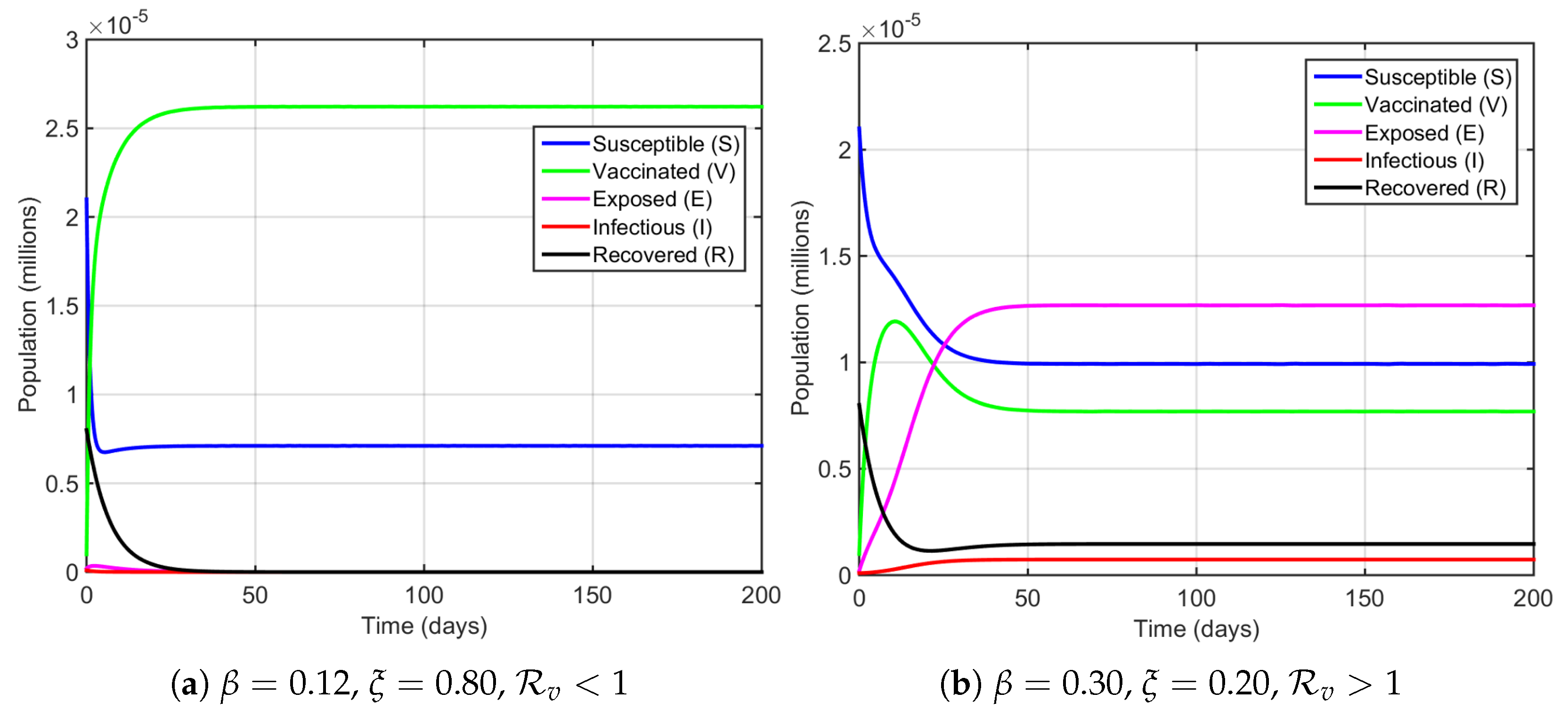
Figure 2 shows the temporal evolution of the SVEIR with reinfection model compartments over 200 days. By using the parameters in Table 1, setting $\beta =0.12$ and $\xi =0.8$, we have ${\mathcal{R}}_v=0.401731<1$. The Jacobian matrix observed in the disease-free equilibrium has eigenvalues of ${\lambda }_1=-0.15;{\lambda }_2=-1.017$, and the other three eigenvalues are negative real numbers since $a_1=0.857950934119961>0,$$a_2=0.170198075909538>0,$$a_3=0.00956668276302851>0$, and $a_1{a}_2-a_3=0.136454915448979>0.$ Based in the Routh–Hurwitz Criterion, the disease-free equilibrium is locally asymptotically stable. Figure 2a illustrates that the solution of the system converges to the disease-free equilibrium point $(7.11242215666994,26.2209111766634,0,0,0)$. This validates that the tuberculosis disease transmission reaches a stable steady-state when ${\mathcal{R}}_v<1$, and the disease will vanish by that time.

Figure 2. Time series of the solution to the TB SVEIR with reinfection model.

However, if we set $\beta =0.3$ and $\xi =0.2$, then we have ${\mathcal{R}}_v=>1$. Thus, again, we have the Jacobian matrix observed in the disease-free equilibrium with eigenvalues ${\lambda }_1=-0.15; {\lambda }_2=-0.417$, and we obtain $a_1=0.422916306954437>0$, $a_2=-0.0544833976019184<0, a_3=-0.0144689463549161<0$, and $a_1{a}_2-a_3=-0.00857297094921750<0.$ Since the Routh–Hurwitz Criterion is not fulfilled, the other three eigenvalues are not all negative real numbers. Therefore, the disease-free equilibrium is not stable when ${\mathcal{R}}_v>1$. Otherwise, the Jacobian matrix evaluated in the endemic equilibrium has eigenvalues of ${\lambda }_1=0, {\lambda }_2=-0.15, {\lambda }_3=-0.417$, and the two other eigenvalues must both be negative real numbers since the quadratic equation ${\lambda }^2+k_1\lambda +k_2=0$ has $k_1=0.494560439560440>0$ and $k_2=0.0497005494505494>0$. This ${\lambda }_1=0$ leads the system to undergo a bifurcation phenomenon. As we obtain $a=-18.9114345094664v_5{w}_5^2<0$ and $b=166.988095238095v_5{w}_5>0$, based on the well-known Center Manifold theorem, the system undergoes a forward bifurcation, which means when $\mathcal{R}>1$, the endemic equilibrium point is locally asymptotically stable, as seen in Figure 2b. This confirms that the tuberculosis disease transmission can be an endemic disease in the system. From Figure 2b, it is seen that the endemic susceptible population $S\left(t\right)$ declines rapidly at the beginning and then stabilizes at a lower level. The vaccinated population $V\left(t\right)$ exhibits a sharp initial increase owing to vaccination and remains dominant in the long term. The exposed class $E\left(t\right)$ grows rapidly during the early phase, surpassing the susceptible population, then gradually settles to a constant level. The infectious population $I\left(t\right)$ rises slightly before reaching a low endemic equilibrium, whereas the recovered class $R\left(t\right)$ decreases sharply at the outset but later increases slowly towards a steady state. These dynamics indicate that the system approaches an endemic equilibrium rather than complete disease eradication.

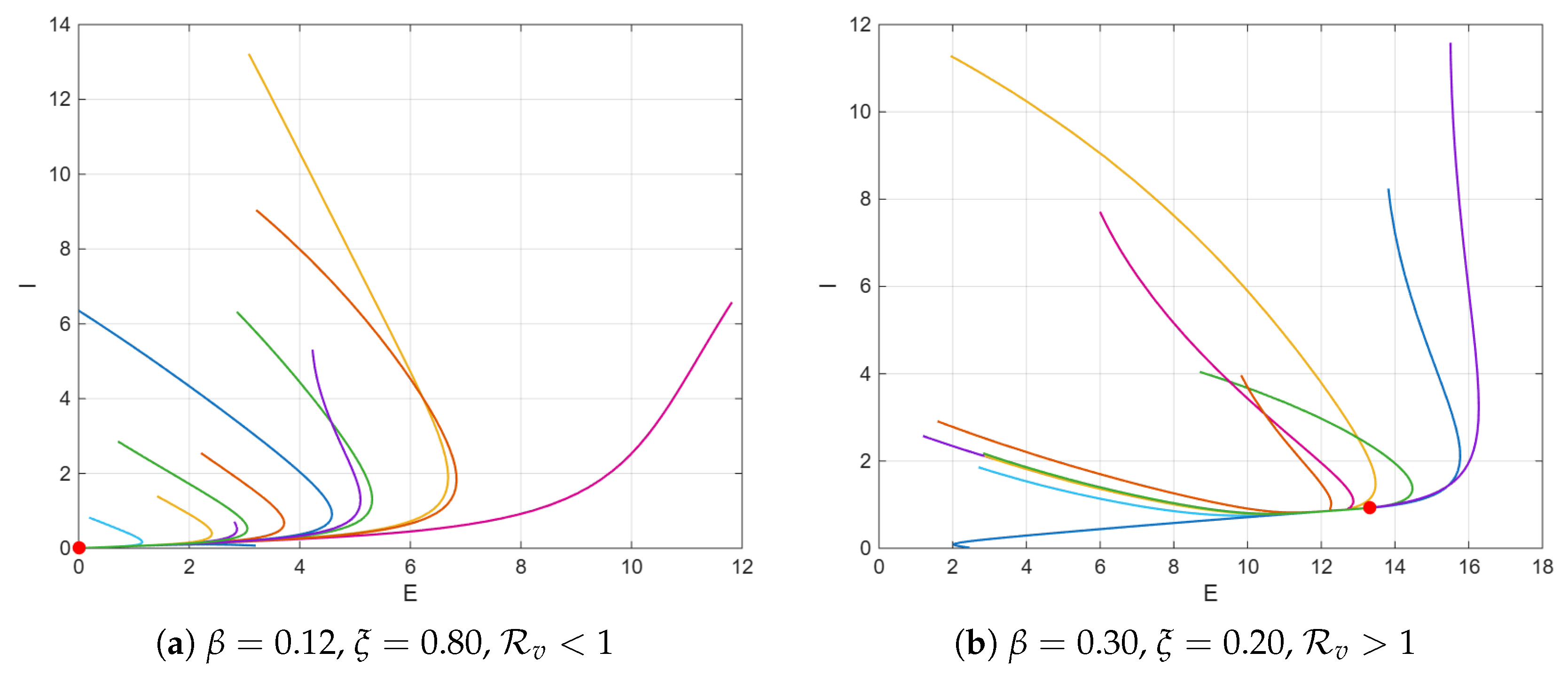
Figure 3 illustrates the phase-plane trajectories of the exposed (E) and infectious (I) populations simulated under diverse initial conditions to verify the global convergence properties of the system (1). The trajectories in Figure 3a correspond to the parameter sets $\beta =0.12$ and $\xi =0.80$, for which ${\mathcal{R}}_v=0.401731<1$. In this regime, all the solution paths monotonically converge toward the origin, indicating that the disease-free equilibrium (DFE) is globally asymptotically stable. This behavior confirms that any initial introduction of infection dies over time when vaccination coverage is sufficiently strong and the transmission rates are low. Conversely, Figure 3b displays the case of $\beta =0.30$ and $\xi =0.20$, yielding ${\mathcal{R}}_v=1.904840>1$. In this regime, all trajectories starting from distinct initial points approach the same positive endemic equilibrium (marked by a red dot), demonstrating global convergence to the endemic steady state.

Figure 3. Phase-plane trajectories in the $(E,I)$-plane from multiple initial conditions showing global convergence of (a) DFE and (b) EE. The red dots denote the corresponding equilibrium points.

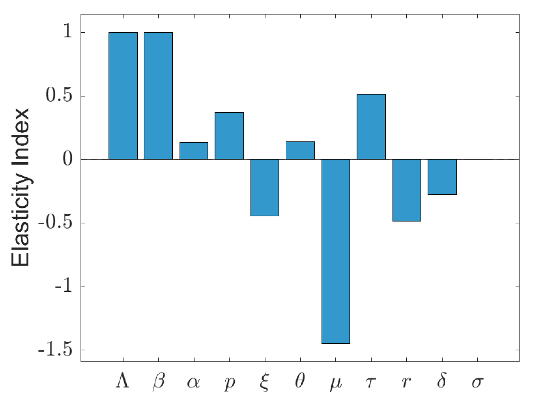
Figure 4 illustrates the elasticity indices of the effective reproduction number ${\mathcal{R}}_v$ for all the model parameters. The recruitment rate ($\Lambda$) and transmission rate ($\beta$) exhibit the highest positive elasticities, implying that increases in these parameters lead to an increase in ${\mathcal{R}}_v$. The progression rate ($\tau$) and the fast-infection fraction (p) also show moderate positive elasticities, while waning immunity ($\theta$) and the vaccine risk reduction factor ($\alpha$) have smaller positive impacts. Conversely, the vaccination rate ($\xi$), recovery rate (r), and disease-induced mortality ($\delta$) display negative elasticities, with the natural death rate ($\mu$) being strongly negative, indicating that an increase in any of these parameters decreases ${\mathcal{R}}_v$. The reinfection parameter ($\sigma$) has slight negative elasticity, suggesting a relatively minor direct influence on ${\mathcal{R}}_v$ in this context. The low elasticity of $\sigma$ supports previous findings [31] that reinfection is less significant than primary infection dynamics.

Figure 4. Elasticity indices of the effective reproduction number ${\mathcal{R}}_v$ with respect to model parameters.

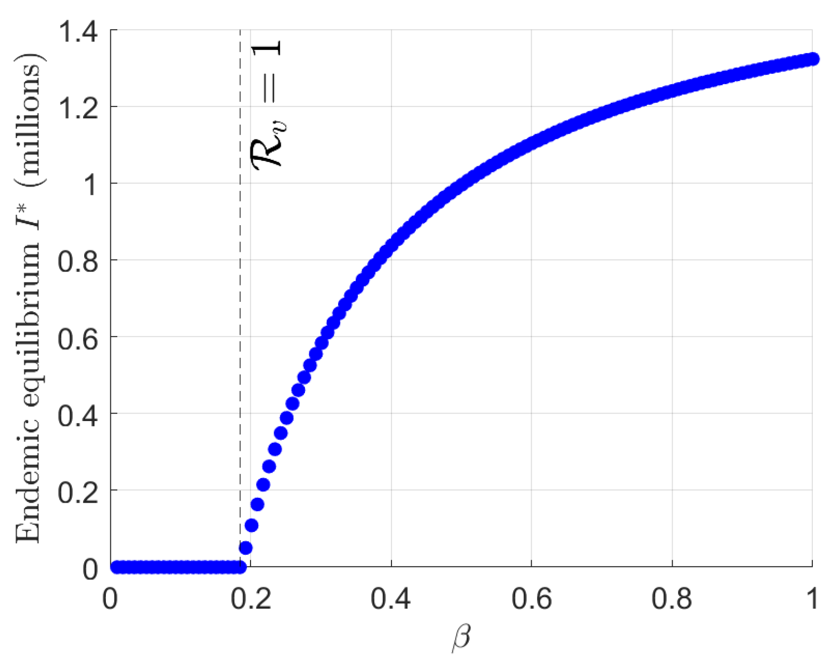
Figure 5 shows that the system (1) underwent the forward bifurcation diagram in the endemic equilibrium $I^{\ast }$ as a function of the transmission rate $\beta$ over the range $[0,1]$. For each $\beta$, the SVEIR with reinfection system was solved numerically using the ode45 solver over a sufficiently long time horizon until convergence to equilibrium, with the final value of $I\left(t\right)$ recorded as $I^{\ast }$. A continuation approach was applied using the equilibrium state from the previous $\beta$ value as the initial condition for the subsequent step. The curve illustrates that $I^{\ast }$ remains zero for $\beta$ below a critical threshold, where ${\mathcal{R}}_v=1$ (dashed vertical line), indicating a stable disease-free equilibrium. As a characteristic of a forward bifurcation, once this threshold is crossed, $I^{\ast }$ increases monotonically with $\beta$, reflecting the emergence and persistence of a stable endemic equilibrium.

Figure 5. Bifurcation diagram of the TB SVEIR with reinfection model with respect to the transmission rate $\beta$.

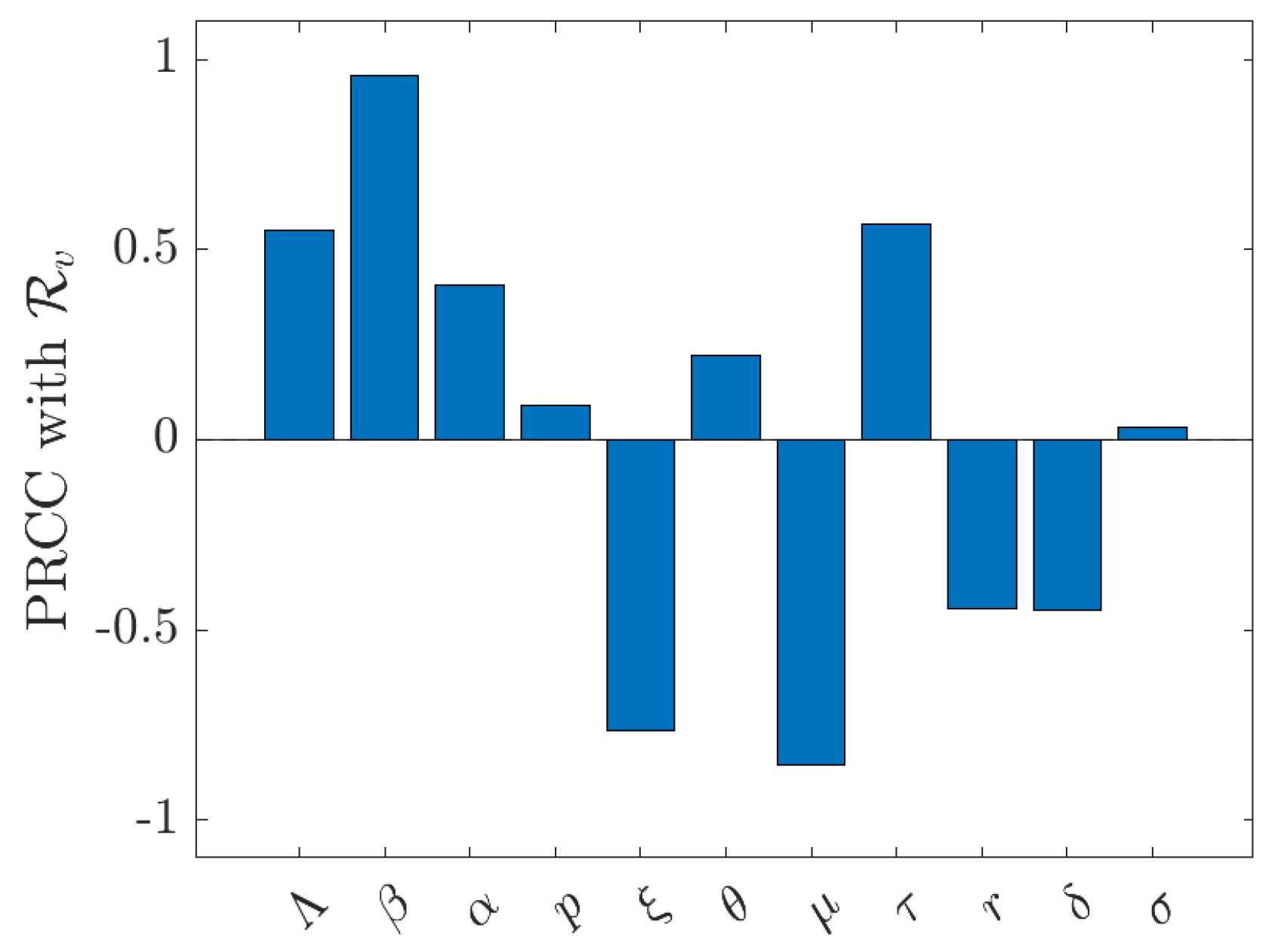
Figure 6 illustrates the partial rank correlation coefficients (PRCCs) derived from Latin Hypercube Sampling with 1000 iterations. Parameter $\beta$ exhibits the most substantial positive correlation, followed by $\Lambda$, aligned with the elasticity findings. The vaccination rate ($\xi$) and the natural death rate ($\mu$) show strong negative PRCCs, whereas r and $\delta$ are moderately negative, emphasizing that vaccination, natural turnover, and recovery reduce the duration of infectiousness and decrease ${\mathcal{R}}_v$. Parameters p and $\sigma$ have weak (near-zero) correlations, suggesting a minimal impact on ${\mathcal{R}}_v$ within the sampled ranges, whereas $\alpha$, $\theta$, and $\tau$ are slightly positive.

Figure 6. Partial rank correlation coefficients (PRCC) of ${\mathcal{R}}_v$ with respect to model parameters.

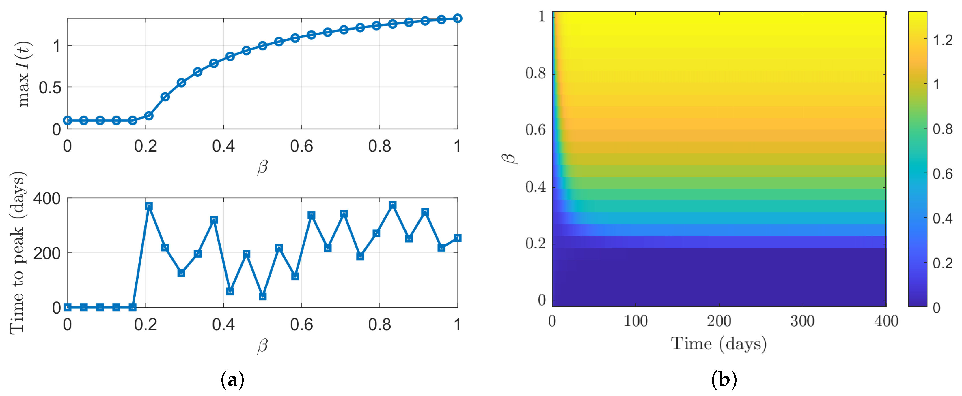
Figure 7 shows how the peak size and timing of the infectious population $I\left(t\right)$ change with the transmission rate $\beta$ in the TB SVEIR with reinfection model. Simulations over 400 days using the ode45 solver indicate that the peak of $I\left(t\right)$ remains close to zero when $\beta$ is below the epidemic threshold but rises steadily as $\beta$ increases past this point. The time to reach the peak jumps sharply just after the threshold and then varies irregularly for higher $\beta$ values. Figure 7b presents a heatmap of $I\left(t\right)$ over time for different $\beta$ values, indicating that higher transmission rates cause larger and more persistent infection peaks. These findings highlight the strong nonlinear effect of $\beta$ on both the severity and timing of an outbreak.

Figure 7. Sensitivity of the infectious class $I\left(t\right)$ to variations in the transmission rate $\beta$: (a) Peak value and timing of $I\left(t\right)$ versus $\beta$. (b) Heatmap of $I\left(t\right)$ over time for varying $\beta$.

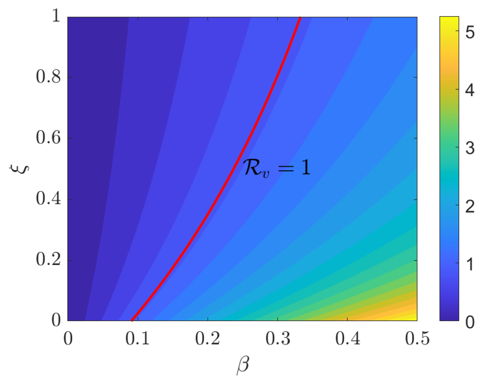
Figure 8 illustrates the contour map of ${\mathcal{R}}_v$ as it varies with $(\beta ,\xi )$, where the red line marks the threshold at ${\mathcal{R}}_v=1$. As $\xi$ increases, this threshold shifts rightward, enlarging the $(\beta ,\xi )$ area, where ${\mathcal{R}}_v<1$. However, an increase in $\beta$ tends to move the system towards ${\mathcal{R}}_v>1$. From an epidemiological perspective, high vaccination levels can counteract transmission pressure; however, the plot reveals that there is no universal, beta-independent vaccination level that ensures ${\mathcal{R}}_v<1$ across the entire range of $\beta$. Instead, for each specific $\beta$ value, there is a corresponding critical vaccination level ${\xi }_{\mathrm{crit}}\left(\beta \right)$, as indicated by the ${\mathcal{R}}_v=1$ contour. Increasing $\xi$ reduces ${\mathcal{R}}_v$ and permits a higher allowable $\beta$ value while remaining within the disease-free zone.

Figure 8. Contour plot of the effective reproduction number ${\mathcal{R}}_v$ as a function of the transmission rate $\beta$ and vaccination rate $\xi$. The red curve represents the threshold ${\mathcal{R}}_v=1$.

5. Discussion

This study focuses on analyzing the dynamics of a tuberculosis disease model that considers imperfect vaccination and a saturated infection rate. The limitation in terms of the saturated rate of this research is that we use the form of saturated logistic incidence rate, ${\displaystyle \frac{1}{1+kI}}$, where k is the parameter that controls the rate of saturation. Therefore, as $I\left(t\right)$ increases, the transmission rate saturates and no longer grows linearly. On the other hand, many researchers also use the saturated rate as ${\displaystyle \frac{1}{A+I}}$, which indicates that as the number of infected individuals $I\left(t\right)$ increases, the transmission rate does not increase linearly but instead approaches a maximum limit as $I\left(t\right)$ reaches the value A. In addition to the disease infection rate, many researchers have also applied the saturated form in the treatment rate [33,34,35].

The effective reproduction number is primarily influenced by the rate of disease transmission, followed by the rate of progression of exposed individuals becoming infected and the rate of fast progression transmission from susceptible individuals becoming infected directly. This suggests that the most effective way to reduce the effective reproduction number is by limiting interactions with infected individuals through public health campaigns, such as social distancing, to prevent widespread transmission of the disease. Another strategy, the rate of vaccination and rate of recovery of infected individuals, as presented in the PRCC analysis in the previous section, was found to have a significant impact. Furthermore, the contour plot highlights and confirms the importance of policymakers recognizing that a combination of disease control measures, vaccination, and treatment can be a crucial solution for reducing tuberculosis transmission.

By construction, the saturated incidence $\beta IS/(1+kI)$ reduces to $\beta IS$ at the disease-free equilibrium; thus, k does not appear in the next-generation matrix. Consequently, both ${\mathcal{R}}_0$ and ${\mathcal{R}}_v$ are analytically invariant with respect to k. Nevertheless, k influences the dynamics away from the DFE; a larger k value decreases the effective force of infection when I is non-negligible, lowering the endemic level and attenuating transient overshoots. Across the biologically plausible range tested, simulations showed monotone or mildly damped approaches to equilibrium and no sustained oscillations, consistent with the absence of treatment saturation or delays in the present model.

For the baseline SVEIR model with saturated incidence and reinfection analyzed here, the transcritical bifurcation at ${\mathcal{R}}_v=1$ is forward, the DFE is globally stable for ${\mathcal{R}}_v<1$, and a unique endemic equilibrium emerges for ${\mathcal{R}}_v>1$. However, backward bifurcation can arise under modified assumptions that intensify the nonlinear competition for control resources or introduce memory effects. Two common mechanisms documented in the literature are: (i) capacity-limited (saturating) treatment or diagnosis, e.g., replacing $rI$ by a concave term, which weakens removal at a higher prevalence, and (ii) time delays in progression or treatment. Both mechanisms are known to generate bistability with a stable DFE coexisting with a stable endemic equilibrium for some ${\mathcal{R}}_v<1$ (see, e.g., [34,35]). Formally, a center-manifold reduction at ${\mathcal{R}}_v=1$ (following [36]) yields bifurcation coefficients $a$ and $b$; where $b>0$, the direction is determined by the sign of $a$. $a>0$ indicates a backward bifurcation, and $a<0$ is a forward bifurcation. In our parameterization (without treatment saturation or delays), numerical continuation and simulations show no evidence of backward bifurcation or multistability, which appears only for ${\mathcal{R}}_v>1$ and is consistent with the forward case.

The forward bifurcation identified at ${\mathcal{R}}_v=1$ implies that tuberculosis elimination is achievable only if the control interventions reduce ${\mathcal{R}}_v$ below unity. Once this threshold is crossed, the disease-free equilibrium becomes globally stable and further control efforts yield monotonically diminishing benefits. This contrasts with backward bifurcation, where ${\mathcal{R}}_v<1$ does not guarantee elimination. Hence, in the present model, maintaining ${\mathcal{R}}_v<1$ through sustained vaccination, early diagnosis, and treatment is necessary and sufficient for eradication.

The inclusion of a saturated transmission rate modifies the perceived impact of vaccination compared to linear incidence models. Under saturation, infection growth slows as the number of infectious individuals increases, reflecting behavioral or contact-limiting effects. Consequently, vaccination and other preventive measures have relatively stronger effects at low to moderate prevalence but diminishing marginal returns at very high infection levels when the contact rate is already constrained. This nonlinear effect highlights the importance of early intervention before the population increases.

Finally, the model with imperfect vaccination (efficacy parameter $0<\alpha <1$) demonstrates that incomplete protection can sustain endemicity, even under high coverage. If vaccine-induced risk reduction is modest or immunity wanes quickly (large $\theta$), ${\mathcal{R}}_v$ may remain above one despite extensive vaccination campaigns. This finding underscores the need for long-lasting vaccines with high efficacy, complemented by non-pharmaceutical interventions that reduce the effective transmission rate $\beta$, to ensure a lasting transition to the disease-free state.

The sensitivity analysis indicates that the effective reproduction number ${\mathcal{R}}_v$ responds strongly to the vaccination rate $\xi$ (negative correlation) and waning-immunity rate $\theta$ (positive correlation). A higher vaccination coverage ($\xi$) markedly lowers ${\mathcal{R}}_v$, emphasizing the importance of sustained immunization programs and improved vaccine access. Conversely, a faster waning of protection ($\theta$) can offset these gains, suggesting that booster doses or longer-lasting vaccines are essential for maintaining population immunity. Overall, effective TB control requires both high coverage and durable immunity because increasing vaccination alone may not ensure elimination if immunity decays rapidly.

6. Conclusions

This study presents a proposed basic tuberculosis SVEIR with reinfection model with imperfect vaccination, considering a saturated infection rate. As a result of imperfect vaccination, we consider that vaccinated individuals can still be infected and move to the exposed class. We assume both fast and slow progress of the infection rate from the susceptible class. The positivity and boundedness of every single solution in this model have been proven. The investigation of the existence of equilibrium points resulted in the existence of two equilibrium points: a disease-free and an endemic equilibrium point. The disease-free equilibrium point exists whenever the effective reproduction number ${\mathcal{R}}_v$ is less than unity. Otherwise, a unique endemic equilibrium point exists if the effective reproduction number is greater than unity. Using linearization, the Jacobian matrix, and the Routh–Hurwitz criterion, we demonstrated that the disease-free equilibrium point is locally asymptotically stable when the effective reproduction number is less than one and satisfies certain conditions. We also analyze the disease-free equilibrium point globally as well by applying the well-known Lyapunov’s Theorem. Using the Center Manifold Theorem, we understood that this model undergoes a forward bifurcation when the effective reproduction number is equal to one, and the endemic equilibrium point is locally stable when the effective reproduction number is greater than one. The numerical simulations showed that the effective reproduction number was inversely proportional to both the rate of saturated infection and the rate of vaccination, whereas it was directly proportional to the rate of disease transmission. These results confirm that the imperfect vaccination strategy model is effective in reducing the transmission of tuberculosis.

In future work, this research can be extended by considering the maximum transmission capacity, ${\displaystyle \frac{1}{A+I}}$ as regulated by the intervention (vaccination program) that limits transmission after the population has been infected. Furthermore, future research could explore a more comprehensive and in-depth analysis of global stability, incorporating advanced techniques and methodologies to improve the understanding of the system’s long-term behavior [30,37]. Furthermore, this research could be explored in the form of fractional-order models, as seen in many other studies on the dynamical analysis of epidemic models [19,37,38,39].

Appendix A.1. The Calculation of Effective Reproduction Number (${\mathcal{R}}_v$)

To compute the effective reproduction number ${\mathcal{R}}_v$, we used the next-generation matrix method considering the infected compartments $E,I$, and R.

We define the following:

$$\mathcal{F}=\left[\begin{array}{c}{\displaystyle \frac{(1-p)\beta SI}{1+kI}}+{\displaystyle \frac{{\beta }_{1}VI}{1+kI}}\\ {\displaystyle \frac{p\beta SI}{1+kI}}\\ 0\end{array}\right],\mathcal{V}=\left[\begin{array}{c}(\tau +\mu )E-\sigma R\\ (r+\delta +\mu )I-\tau E\\ (\sigma +\mu )R-rI\end{array}\right].$$

(A1)

In the DFE, we linearize around $P^0=(S^0,V^0,0,0,0)$. The Jacobian matrices of $\mathcal{F}$ and $\mathcal{V}$ with respect to $(E,I,R)$ are

$$F=\left[\begin{array}{ccc}0& (1-p)\beta S^0+{\beta }_1{V}^0& 0\\ 0& p\beta S^0& 0\\ 0& 0& 0\end{array}\right],V=\left[\begin{array}{ccc}\tau +\mu & 0& -\sigma \\ -\tau & r+\delta +\mu & 0\\ 0& -r& \sigma +\mu \end{array}\right].$$

Then, the effective reproduction number is given by ${\mathcal{R}}_v=\rho \left(F{V}^{-1}\right)$, where $\rho (·)$ denotes the spectral radius (dominant eigenvalue) of the matrix. The result is

$${\mathcal{R}}_v={\displaystyle \frac{(\sigma +\mu )A_1}{A_2{A}_3}},$$

where $A_1=\Lambda \left[(\theta +\mu )(\tau +\mu p)\beta +{\beta }_1\tau \xi \right]$, $A_2=[(\tau +\mu )(r+\mu +\delta )(\sigma +\mu )-\tau r\sigma ]$, and $A_3=\mu (\xi +\mu +\theta )$.

Appendix A.2. Proof of Local Stability of DFE in Theorem 3

Proof. 

The Jacobian matrix of system (1) is given as follows:

$$J=\left[\begin{array}{ccccc}-{\displaystyle \frac{\beta I}{1+kI}}-\xi -\mu & \theta & 0& -{\displaystyle \frac{\beta S}{{(1+kI)}^2}}& 0\\ \xi & -{\displaystyle \frac{{\beta }_{1}I}{1+kI}}-\theta -\mu & 0& -{\displaystyle \frac{{\beta }_{1}V}{{(1+kI)}^2}}& 0\\ {\displaystyle \frac{(1-p)\beta I}{1+kI}}& {\displaystyle \frac{{\beta }_{1}I}{1+kI}}& -\tau -\mu & {\displaystyle \frac{(1-p)\beta S}{{(1+kI)}^2}}+{\displaystyle \frac{{\beta }_{1}V}{{(1+kI)}^2}}& \sigma \\ {\displaystyle \frac{p\beta I}{1+kI}}& 0& \tau & {\displaystyle \frac{p\beta S}{{(1+kI)}^2}}-r-\delta -\mu & 0\\ 0& 0& 0& r& -(\sigma +\mu )\end{array}\right].$$

(A2)

At the DFE, $I=0$, $E=0$, and $R=0$, the Jacobian (A2) simplifies to the following:

$$J_{\mathrm{DFE}}=\left[\begin{array}{ccccc}-\xi -\mu & \theta & 0& -{\displaystyle \frac{\beta (\theta +\mu )\Lambda }{\mu (\xi +\mu +\theta )}}& 0\\ \xi & -\theta -\mu & 0& -{\displaystyle \frac{{\beta }_1\Lambda \xi }{\mu (\xi +\mu +\theta )}}& 0\\ 0& 0& -\tau -\mu & {\displaystyle \frac{(1-p)\beta (\theta +\mu )\Lambda }{\mu (\xi +\mu +\theta )}}+{\displaystyle \frac{{\beta }_1\Lambda \xi }{\mu (\xi +\mu +\theta )}}& \sigma \\ 0& 0& \tau & {\displaystyle \frac{p\beta (\theta +\mu )\Lambda }{\mu (\xi +\mu +\theta )}}-r-\delta -\mu & 0\\ 0& 0& 0& r& -(\sigma +\mu )\end{array}\right].$$

Thus, the eigenvalues of the Jacobian matrix at the DFE are

$${\lambda }_1=-\mu ,{\lambda }_2=-\xi -\mu -\theta ,$$

while the remaining three eigenvalues are obtained by solving this 3 by 3 matrix as follows:

$$A=\left[\begin{array}{ccc}-\tau -\mu & {\displaystyle \frac{(1-p)\beta \Lambda (\theta +\mu )}{A_3}}+{\displaystyle \frac{{\beta }_1\Lambda \xi }{A_3}}& \sigma \\ \tau & {\displaystyle \frac{p\beta \Lambda (\theta +\mu )}{A_3}}-r-\delta -\mu & 0\\ 0& r& -\sigma -\mu \end{array}\right]$$

The following characteristic equation is obtained:

$${\lambda }^3+a_1{\lambda }^2+a_2\lambda +a_3=0.$$

(A3)

Based on (A3), the eigenvalues of matrix A are negative if the following Routh–Hurwitz criterion is satisfied as follows:

• $a_1>0$,
• $a_3>0$,
• $a_1{a}_2>a_3$.

We have

$$\begin{array}{cc}\hfill a_1& ={\displaystyle \frac{(1-{\mathcal{R}}_v)A_2{A}_3+\left[(\theta +\mu )\beta +{\beta }_1\xi \right]\tau \Lambda (\sigma +\mu )+A_3\left[(\sigma +\mu )(2{\mu }^2+\sigma \mu -\tau (r+\delta ))+\tau r\sigma \right]}{A_3(\sigma +\mu )\mu }},\hfill \\ \hfill a_2& ={\displaystyle \frac{(1-{\mathcal{R}}_v)A_2{A}_3(2\mu +\sigma )+{(\sigma +\mu )}^2\Lambda \tau \left((\theta +\mu )\beta +{\beta }_1\xi \right)+A_3\left({(\sigma +\mu )}^2(-\delta \tau +{\mu }^2)-{\mu }^{2}r\tau \right)}{A_3(\sigma +\mu )\mu }},\hfill \\ \hfill a_3& =(1-{\mathcal{R}}_v)A_2.\hfill \end{array}$$

This implies that

$$\begin{array}{cc}\hfill a_1{a}_2-a_3& ={\displaystyle \frac{1}{A_3^2}}\left(p\beta (\theta +\mu )\left(\beta (\theta +\mu )(2\mu p+p\sigma +\tau )+{\beta }_1\tau \xi \right){\Lambda }^2\right)\hfill \\ \hfill & {\displaystyle \frac{(1-{\mathcal{R}}_v)A_2{A}_3(\delta +2\mu +r+\tau )}{A_3(\sigma +\mu )}}+{\displaystyle \frac{(1-{\mathcal{R}}_v)A_2(2\mu +\sigma )(2\delta +4\mu +2r+\sigma )}{\mu (\sigma +\mu )}}\hfill \\ \hfill & +{\displaystyle \frac{\Lambda (\theta +\mu )(\sigma +\mu )\beta }{A_3\mu (\sigma +\mu )}}[\mu (\delta \mu +2{\mu }^2+\mu r)p+\mu (\delta \tau +3\mu \tau +r\tau +2\sigma \tau )(1-p)\hfill \\ & +\tau \mu (3\delta +5\mu +3r)+\tau \sigma (2\delta +4\mu +2r+\sigma )]+{\displaystyle \frac{A_4\mu (\sigma +\mu )-A_2{A}_5}{\mu (\sigma +\mu )}}\hfill \\ \hfill & +{\displaystyle \frac{\Lambda {\beta }_1\tau \xi (\sigma +\mu )(2\mu +\sigma )(2\delta +4\mu +2r+\sigma )}{A_3\mu (\sigma +\mu )}},\hfill \end{array}$$

with

$A_4=(2\mu +\sigma +\tau ){\delta }^2+(2\mu +\sigma +\tau )(4\mu +2r+\sigma +\tau )\delta +(4{\mu }^2+2\mu r+2\mu \sigma +2\mu \tau +r\sigma +r\tau +\sigma \tau )(\tau +2\mu +r+\sigma )$ and $A_5=\left(5\mu +2\sigma \right)\delta +10{\mu }^2+\left(5r+6\sigma +\tau \right)\mu +\sigma \left(2r+\sigma \right)$.

Based on the following conditions

$$\begin{array}{cc}\hfill 2{\mu }^2+\sigma \mu & >\tau (r+\delta ),\hfill \\ \hfill A_4\mu (\sigma +\mu )& >A_2{A}_5,\hfill \end{array}$$

(A4)

and if ${\mathcal{R}}_v<1$, we obtain $a_1,a_3>0$ and $a_1{a}_2-a_3>0$. Therefore, based on the Routh–Hurwitz conditions, we conclude that the DFE equilibrium point is locally asymptotically stable if ${\mathcal{R}}_v<1$ and if the condition in Equation (A4) is satisfied. □

Appendix A.3. Proof of Global Stability of DFE in Theorem 4

Proof. 

Based on the assumed positivity and boundedness, all trajectories starting in $\Omega$ remain in $\Omega$. Moreover, from the $(S,V)$-subsystem

$${\displaystyle \frac{dS}{dt}}=\Lambda +\theta V-{\displaystyle \frac{\beta IS}{1+kI}}-(\xi +\mu )S,{\displaystyle \frac{dV}{dt}}=\xi S-{\displaystyle \frac{{\beta }_{1}VI}{1+kI}}-(\theta +\mu )V,$$

and since the incidence terms are non-negative, standard comparison with the linear system

$${\displaystyle \frac{dS}{dt}}=\Lambda +\theta V-(\xi +\mu )S,{\displaystyle \frac{dV}{dt}}=\xi S-(\theta +\mu )V$$

implies for all $t\ge 0$ that

$$S\left(t\right)\le S^0,V\left(t\right)\le V^0,{\displaystyle \frac{S\left(t\right)}{1+kI\left(t\right)}}\le S^0,{\displaystyle \frac{V\left(t\right)}{1+kI\left(t\right)}}\le V^0.$$

(A5)

We define a linear Lyapunov function on the “infected” variables $(E,I,R)$:

$$L(E,I,R)={\theta }_{1}E+I+{\theta }_{2}R,{\theta }_1:={\displaystyle \frac{\tau }{\tau +\mu }},{\theta }_2:={\displaystyle \frac{{\theta }_1\sigma }{\sigma +\mu }}={\displaystyle \frac{\tau \sigma }{(\tau +\mu )(\sigma +\mu )}}.$$

Clearly $L\ge 0$ on $\Omega$ and $L=0$ iff $(E,I,R)=(0,0,0)$. Along solutions of (1),

$$\begin{array}{cc}\hfill {\displaystyle \frac{dL}{dt}}& ={\theta }_1{\displaystyle \frac{dE}{dt}}+{\displaystyle \frac{dI}{dt}}+{\theta }_2{\displaystyle \frac{dR}{dt}}\hfill \\ \hfill & ={\theta }_1\left({\displaystyle \frac{(1-p)\beta SI}{1+kI}}+{\displaystyle \frac{{\beta }_{1}VI}{1+kI}}+\sigma R-(\tau +\mu )E\right)+\left({\displaystyle \frac{p\beta SI}{1+kI}}+\tau E-(r+\delta +\mu )I\right)\hfill \\ \hfill & +{\theta }_2\left(rI-(\sigma +\mu )R\right)\hfill \\ \hfill & =\underset{=0}{\underbrace{\left(-{\theta }_1(\tau +\mu )+\tau \right)}}E+\underset{=0}{\underbrace{\left({\theta }_1\sigma -{\theta }_2(\sigma +\mu )\right)}}R\hfill \\ \hfill & +\left[\left({\theta }_1(1-p)+p\right)\beta {\displaystyle \frac{S}{1+kI}}+{\theta }_1{\beta }_1{\displaystyle \frac{V}{1+kI}}+r({\theta }_2-1)-(\delta +\mu )\right]I.\hfill \end{array}$$

Using the bounds (A5) yields the following:

$${\displaystyle \frac{dL}{dt}}\le \left[\left({\theta }_1(1-p)+p\right)\beta S^0+{\theta }_1{\beta }_1{V}^0+r({\theta }_2-1)-(\delta +\mu )\right]I.$$

A direct algebraic simplification, using

$${\theta }_3=(\tau +\mu )(r+\delta +\mu )(\sigma +\mu )-\tau r\sigma >0,$$

and Formula (5) for ${\mathcal{R}}_v$, gives

$$\left({\theta }_1(1-p)+p\right)\beta S^0+{\theta }_1{\beta }_1{V}^0+r({\theta }_2-1)-(\delta +\mu )=-{\displaystyle \frac{{\theta }_3}{(\tau +\mu )(\sigma +\mu )}}\left(1-{\mathcal{R}}_v\right).$$

Therefore,

$${\displaystyle \frac{dL}{dt}}\le -{\displaystyle \frac{{\theta }_3}{(\tau +\mu )(\sigma +\mu )}}\left(1-{\mathcal{R}}_v\right)I\le 0,$$

with equality only when $I=0$, which, together with the cancellations above, implies $E=R=0$. According to LaSalle’s invariance principle, the largest invariant subset of $\{dL/dt=0\}$ in $\Omega$ is the singleton, $\{(S,V,E,I,R)=(S^0,V^0,0,0,0)\}$. Hence, the DFE is globally asymptotically stable in $\Omega$ whenever ${\mathcal{R}}_v<1$. □

Appendix A.4. Proof of Forward Bifurcation in Theorem 6

Proof. 

We now examine the behavior of system (1) when ${\mathcal{R}}_v$ approaches unity. Note that ${\beta }_1=\alpha \beta$ with $0<\alpha <1$, ${\mathcal{R}}_v$ equals 1 when $\beta$ is set to ${\beta }^{\ast }$. Here, ${\beta }^{\ast }$ is defined as follows:

$${\beta }^{\ast }={\displaystyle \frac{A_2{A}_3}{\Lambda (\mu +\sigma )\left[(\theta +\mu )(\tau +\mu p)+\alpha \tau \xi \right]}}.$$

When $\beta$ is equal to ${\beta }^{\ast }$, characteristic Equation (A2) is expressed as follows:

$$\lambda (\lambda +\mu )(\lambda +\xi +\mu +\theta )K\left(\lambda \right)=0$$

(A6)

where $K\left(\lambda \right)={\lambda }^2+k_1\lambda +k_2$, with

$$\begin{array}{cc}\hfill k_1=& {\displaystyle \frac{1}{B_3(\sigma +\mu )}}[(\theta +\mu )[(2{\mu }^3+3{\mu }^2\sigma +\mu {\sigma }^2)p+(\delta \mu \tau +\delta \sigma \tau +\mu r\tau )(1-p)\hfill \\ \hfill & +\tau \sigma (3\mu +r+\tau +\sigma )+\tau \mu (3\mu +\tau +\sigma )]+\alpha \xi \tau (\sigma +\mu \left)\right(3\mu +r+\tau +\delta +\sigma \left)\right],\hfill \end{array}$$

$$\begin{array}{cc}\hfill k_2=& {\displaystyle \frac{1}{B_3(\sigma +\mu )}}[\alpha \xi \tau \left[({\mu }^2+2\mu \sigma +r\sigma +{\sigma }^2)\tau +{(\mu +\sigma )}^2(\delta +2\mu +r)\right]\hfill \\ & +(\theta +\mu )\left[({\mu }^4+2{\mu }^3\sigma +{\mu }^2{\sigma }^2\right)p+\left(\tau {(\mu +\sigma )}^2\delta +{\mu }^{2}r\tau \right)(1-p)\hfill \\ \hfill & +\tau \left((2\mu +r+\tau ){\sigma }^2+(2\mu +\tau )(2\mu +r)\sigma +{\mu }^2(2\mu +\tau )\right)\left]\right].\hfill \end{array}$$

It is clear that the characteristic equation in (A6) has a simple zero eigenvalue, ${\lambda }_1=0$, and two negative eigenvalues, ${\lambda }_2=-\mu$ and ${\lambda }_3=-(\xi +\mu +\theta )$. Meanwhile, because $k_1$ and $k_2$ are both positive, the other eigenvalues must be negative; that is, ${\lambda }_4,{\lambda }_5\in {\mathbb{R}}^{-}$. The right eigenvector of $J_{(E_0,{\beta }^{\ast })}$, which corresponds to the zero eigenvalue ${\lambda }_1=0$, is

$$\overrightarrow{w}=\left[\begin{array}{ccccc}-{\displaystyle \frac{A_2{w}_5{B}_1}{A_3{B}_{3}r}}& - {\displaystyle \frac{A_2\xi w_5{B}_2}{A_3{B}_{3}r}}& {\displaystyle \frac{w_5\left[A_2\alpha \xi +A_2(\mu +\theta )(1-p)+B_{3}r\sigma \right]}{B_{3}r(\sigma +\mu )}}& {\displaystyle \frac{w_5(\sigma +\mu )}{r}}& w_5\end{array}\right]$$

where $B_1=\alpha \xi \theta +{\mu }^2+2\mu \theta +{\theta }^2$, $B_2=\alpha \xi +\alpha \mu +\mu +\theta$ and $B_3=\alpha \xi \tau +{\mu }^{2}p+\mu p\theta +\tau \mu +\tau \theta$, and $w_5$ are positive constants. The left eigenvector of $J_{(E_0,{\beta }^{\ast })}$ that corresponds to ${\lambda }_1=0$ is

$$\overrightarrow{v}={\left[\begin{array}{ccccc}0& 0& {\displaystyle \frac{v_5(\sigma +\mu )}{\sigma }}& {\displaystyle \frac{v_5({\mu }^2+\mu \sigma +\mu \tau +\sigma \tau )}{\tau \sigma }}& v_5\end{array}\right]}^T$$

where $v_5$ is selected such that $\overrightarrow{w}·\overrightarrow{v}=1$. This gives

$$\begin{array}{cc}\hfill w_5=& (A_2\tau (\mu +\sigma )\left[\alpha \xi +(\mu +\theta )(1-p)\right]\hfill \\ & +B_3\left[{\sigma }^2[\tau r+{(\tau +\mu )}^2]+\sigma [\tau r(2\mu +\tau )+2\mu {(\tau +\mu )}^2]+{\mu }^2{(\tau +\mu )}^2\right]{)}^{-1}>0,\hfill \\ \hfill v_5=& B_3\sigma r\tau (\tau +\mu )>0.\hfill \end{array}$$

Let $x_1=S, x_2=V, x_3=E, x_4=I, x_5=R$ and $f_1={\displaystyle \frac{\partial S}{\partial t}}, f_2={\displaystyle \frac{\partial V}{\partial t}}, f_3={\displaystyle \frac{\partial E}{\partial t}}, f_4={\displaystyle \frac{\partial I}{\partial t}}, f_5={\displaystyle \frac{\partial R}{\partial t}}$. Clearly, it can be demonstrated that

$$\begin{array}{cc}\hfill a=& \sum _{k,i,j=1}^5{v}_k{w}_i{w}_j{\displaystyle \frac{{\partial }^2{f}_k}{\partial x_i\partial x_j}}(0,0)\hfill \\ \hfill =& -{\displaystyle \frac{2{(\sigma +\mu )}^2{A}_2{B}_1(1-p)\beta v_5{w}_5^2}{\sigma A_3{B}_3{r}^2}}-{\displaystyle \frac{2{(\sigma +\mu )}^2{A}_2\xi B_2\alpha \beta v_5{w}_5^2}{\sigma A_3{B}_3{r}^2}}\hfill \\ & -{\displaystyle \frac{2{(\sigma +\mu )}^3\beta \Lambda k\left((1-p)(\theta +\mu )+\alpha \xi \right)v_5{w}_5^2}{A_3\sigma r^2}}-{\displaystyle \frac{2({\mu }^2+\mu \sigma +\mu \tau +\sigma \tau )(\sigma +\mu )A_{2}p\beta B_1{v}_5{w}_5^2}{\tau \sigma A_3{B}_3{r}^2}}\hfill \\ & -{\displaystyle \frac{2({\mu }^2+\mu \sigma +\mu \tau +\sigma \tau ){(\sigma +\mu )}^{2}p\beta \Lambda (\theta +\mu )k{v}_5{w}_5^2}{\tau \sigma A_3{r}^2}}<0,\hfill \\ \hfill b=& \sum _{k,i=1}^5{v}_k{w}_i{\displaystyle \frac{{\partial }^2{f}_k}{\partial x_i\partial {\beta }^{\ast }}}(0,0)\hfill \\ \hfill =& {\displaystyle \frac{\left[(1-p)(\theta +\mu )+\alpha \xi \right]\Lambda {(\sigma +\mu )}^2{v}_5{w}_5}{A_3\sigma r}}+{\displaystyle \frac{p\Lambda (\theta +\mu )\left({\mu }^2+\mu \sigma +\mu \tau +\sigma \tau \right)(\sigma +\mu )v_5{w}_5}{A_3\tau \sigma r}}>0.\hfill \end{array}$$

Given that $a<0$ and $b>0$, the renowned Center Manifold theorem, as referenced in [36], indicates that a forward bifurcation occurs at ${\mathcal{R}}_v=1$. This suggests that when ${\mathcal{R}}_v>1$, the disease-free equilibrium is unstable, whereas the endemic equilibrium is locally asymptotically stable. □

References

1. Whang, S.; Choi, S.; Jung, E. A dynamic model for tuberculosis transmission and optimal treatment strategies in South Korea. J. Theor. Biol. 2011, 279, 120–131. [Google Scholar] [CrossRef]
2. Peter, O.J.; Aldila, D.; Ayoola, T.A.; Balogun, G.B.; Oguntolu, F.A. Modeling tuberculosis dynamics with vaccination and treatment strategies. Sci. Afr. 2025, 28, e02647. [Google Scholar] [CrossRef]
3. World Health Organization. Global Tuberculosis Report 2018; World Health Organization: Geneva, Switzerland, 2018; Available online: https://www.who.int/publications-detail-redirect/9789241565646 (accessed on 29 August 2025).
4. Sulayman, F.; Abdullah, F.A.; Mohd, M.H. An SVEIRE model of tuberculosis to assess the effect of an imperfect vaccine and other exogenous factors. Mathematics 2021, 9, 327. [Google Scholar] [CrossRef]
5. Harris, R.C.; Sumner, T.; Knight, G.M.; White, R.G. Systematic review of mathematical models exploring the epidemiological impact of future TB vaccines. Hum. Vaccin. Immunother. 2016, 12, 2813–2832. [Google Scholar] [CrossRef]
6. Brennan, M.J.; Stone, M.R.; Evans, T. A rational vaccine pipeline for tuberculosis. Int. J. Tuberc. Lung Dis. 2012, 16, 1566–1573. [Google Scholar] [CrossRef] [PubMed]
7. Fuller, N.M.; McQuaid, C.F.; Harker, M.J.; Weerasuriya, C.K.; McHugh, T.D.; Knight, G.M. Mathematical models of drug-resistant tuberculosis lack bacterial heterogeneity: A systematic review. PLoS Pathog. 2024, 20, e1011574. [Google Scholar] [CrossRef]
8. Wu, Y.; Huang, M.; Wang, X.; Li, Y.; Jiang, L.; Yuan, Y. The prevention and control of tuberculosis: An analysis based on a tuberculosis dynamic model derived from the cases of Americans. BMC Public Health 2020, 20, 1173. [Google Scholar] [CrossRef] [PubMed]
9. Ahmad, Y.U.; Andrawus, J.; Ado, A.; Maigoro, Y.A.; Yusuf, A.; Althobaiti, S.; Mustapha, U.T. Mathematical modeling and analysis of human-to-human monkeypox virus transmission with post-exposure vaccination. Model. Earth Syst. Environ. 2024, 10, 2711–2731. [Google Scholar] [CrossRef]
10. Rajan, P.K.; Kuppusamy, M.; Yusuf, A. A fractional-order modeling of human papillomavirus transmission and cervical cancer. Model. Earth Syst. Environ. 2024, 10, 1337–1357. [Google Scholar] [CrossRef]
11. Öztürk, B.A.; Yusuf, A.; Inc, M. Fractional HIV infection model described by the Caputo derivative with real data. Bol. Soc. Mat. Mex. 2024, 30, 1–23. [Google Scholar] [CrossRef]
12. Al-Shomrani, M.M.; Musa, S.S.; Yusuf, A. Unfolding the transmission dynamics of monkeypox virus: An epidemiological modeling analysis. Mathematics 2023, 11, 1121. [Google Scholar] [CrossRef]
13. Lee, S.; Park, H.-Y.; Ryu, H.; Kwon, J.-W. Age-specific mathematical model for tuberculosis transmission dynamics in South Korea. Mathematics 2021, 9, 804. [Google Scholar] [CrossRef]
14. Saber, S.; Dridi, B.; Alahmari, A.; Messaoudi, M. Hyers–Ulam stability and control of fractional glucose–insulin systems. Eur. J. Pure Appl. Math. 2025, 18, 6152. [Google Scholar] [CrossRef]
15. Alhazmi, M.; Saber, S. Application of a fractal–fractional derivative with a power-law kernel to the glucose–insulin interaction system based on Newton’s interpolation polynomials. Fractals 2025. [Google Scholar] [CrossRef]
16. Trauer, J.M.; Denholm, J.T.; McBryde, E.S. Construction of a mathematical model for tuberculosis transmission in highly endemic regions of the Asia-Pacific. J. Theor. Biol. 2014, 358, 74–84. [Google Scholar] [CrossRef]
17. Qiu, Z.; Feng, Z. Transmission dynamics of an influenza model with vaccination and antiviral treatment. Bull. Math. Biol. 2010, 72, 1–33. [Google Scholar] [CrossRef]
18. Ahmad, S.; Pak, S.; Rahman, M.U.; Al-Bossly, A. On the analysis of a fractional tuberculosis model with the effect of an imperfect vaccine and exogenous factors under the Mittag–Leffler kernel. Fractal Fract. 2023, 7, 526. [Google Scholar] [CrossRef]
19. Nandi, T.R.; Saha, A.K.; Roy, S. Analysis of a fractional order epidemiological model for tuberculosis transmission with vaccination and reinfection. Sci. Rep. 2024, 14, 28290. [Google Scholar] [CrossRef] [PubMed]
20. Saputra, H.L.; Darti, I.; Suryanto, A. Analysis of SVEIL model of tuberculosis disease spread with imperfect vaccination. J. Teor. Apl. Mat. 2023, 7, 125–135. [Google Scholar] [CrossRef]
21. Zhang, J.; Jia, J.; Song, X. Analysis of an SEIR epidemic model with saturated incidence and saturated treatment function. Sci. World J. 2014, 2014, 910421. [Google Scholar] [CrossRef] [PubMed]
22. Baba, I.A.; Abdulkadir, R.A.; Esmaili, P. Analysis of tuberculosis model with saturated incidence rate and optimal control. Phys. A Stat. Mech. Appl. 2020, 540, 123237. [Google Scholar] [CrossRef]
23. Bentaleb, D.; Harroudi, S.; Amine, S.; Allali, K. Analysis and optimal control of a multistrain SEIR epidemic model with saturated incidence rate and treatment. Differ. Equ. Dyn. Syst. 2023, 31, 907–923. [Google Scholar] [CrossRef]
24. Capasso, V.; Serio, G. A generalization of the Kermack–McKendrick deterministic epidemic model. Math. Biosci. 1978, 42, 43–61. [Google Scholar] [CrossRef]
25. Witbooi, P.J.; Mengistu, A.K. Mathematical analysis of TB model with vaccination and saturated incidence rate. Abstr. Appl. Anal. 2020, 2020, 6669997. [Google Scholar] [CrossRef]
26. Rasheed, S.; Iyiola, O.S.; Oke, S.I.; Wade, B.A. Exploring a mathematical model with saturated treatment for the co-dynamics of tuberculosis and diabetes. Mathematics 2024, 12, 3765. [Google Scholar] [CrossRef]
27. Lu, M.; Huang, J.; Ruan, S.; Yu, P. Bifurcation analysis of an SIRS epidemic model with a generalized nonmonotone and saturated incidence rate. J. Differ. Equ. 2019, 267, 1859–1898. [Google Scholar] [CrossRef] [PubMed]
28. Mengistu, A.K.; Witbooi, P.J. Modeling the effects of vaccination and treatment on tuberculosis transmission dynamics. J. Appl. Math. 2019, 1, 7463167. [Google Scholar] [CrossRef]
29. Kar, T.K.; Mondal, P.K. Global dynamics of a tuberculosis epidemic model and the influence of backward bifurcation. J. Math. Model. Algorithms 2012, 11, 433–459. [Google Scholar] [CrossRef]
30. Egonmwan, A.O.; Okuonghae, D. Mathematical analysis of a tuberculosis model with imperfect vaccine. Int. J. Biomath. 2019, 12, 1950040. [Google Scholar] [CrossRef]
31. Horsburgh, C.R.; Jo, Y.; Nichols, B.; Jenkins, H.E.; Russell, C.A.; White, L.F. Contribution of Reinfection to Annual Rate of Tuberculosis Infection (ARI) and Incidence of Tuberculosis Disease Free. Clin. Infect. Dis. 2023, 76, e965–e972. [Google Scholar] [CrossRef]
32. Ragonnet, R.; Flegg, J.A.; Brilleman, S.L.; Tiemersma, E.W.; Melsew, Y.A.; McBryde, E.S.; Trauer, J.M. Revisiting the natural history of pulmonary tuberculosis: A Bayesian estimation of natural recovery and mortality rates. Clin. Infect. Dis. 2021, 73, e88–e96. [Google Scholar] [CrossRef]
33. Sulayman, F.; Abdullah, F. Analysis of a Tuberculosis Infection Model considering the Influence of Saturated Recovery (Treatment). Complex 2021, 2021, 1805651:1–1805651:16. [Google Scholar] [CrossRef]
34. Aldila, D.; Saslia, B.R.; Gayarti, W.; Tasman, H. Backward bifurcation analysis on Tuberculosis disease transmission with saturated treatment. J. Phys. Conf. Ser. 2021, 1821, 012002. [Google Scholar] [CrossRef]
35. Zhou, L.; Fan, M. Dynamics of an SIR epidemic model with limited medical resources revisited. Nonlinear Anal. Real World Appl. 2012, 13, 312–324. [Google Scholar] [CrossRef]
36. Castillo-Chavez, C.; Song, B. Dynamical models of tuberculosis and their applications. Math. Biosci. Eng. 2004, 1, 361–404. [Google Scholar] [CrossRef]
37. Khan, M.A.; DarAssi, M.H.; Ahmad, I.; Seyam, N.M.; Alzahrani, E. Modeling the Dynamics of Tuberculosis with Vaccination, Treatment, and Environmental Impact: Fractional Order Modeling. Comput. Model. Eng. Sci. 2024, 141, 1365–1394. [Google Scholar] [CrossRef]
38. Gemeda, A.E.; Obsu, L.L.; Gurmu, E.D. Mathematical modeling of tuberculosis transmission dynamics with vaccination and two lines of treatments: A Caputo fractional approach. J. Appl. Math. Comput. 2025, 71, 2017–2049. [Google Scholar] [CrossRef]
39. Amilo, D. Analyzing the Dynamics of Tuberculosis through a Fractional-Order Model. J. Math. Model. Fract. Calc. 2024. [Google Scholar] [CrossRef]