Mathematical Insights into the Spatio-Temporal Dynamics of Vector-Borne Diseases in Tropical Regions

Abstract

Vector-borne diseases pose a significant public health challenge in tropical regions, where complex interactions between hosts, vectors, and the environment drive epidemic dynamics. In this study, we develop a spatio-temporal mathematical model to describe the spread of such diseases, incorporating population dynamics and spatial–temporal factors affecting pathogen transmission. We conduct a theoretical analysis of the model, proving the existence, uniqueness, and positivity of solutions. Additionally, we examine equilibrium states and key epidemiological parameters, including the basic reproduction number. Our findings provide mathematical insights into epidemic propagation and offer a foundation for designing effective control strategies.

1. Introduction

Infectious diseases have consistently posed a major challenge to global health, necessitating continuous efforts to understand and mitigate their spread. The emergence and re-emergence of novel pathogens highlight the importance of developing robust epidemiological models that can effectively capture the underlying mechanisms of disease transmission. The readers can refer to [1,2,3] and references theirin. While traditional approaches based on ordinary differential equations (ODEs) have provided valuable insights, they often fail to account for spatial heterogeneity and migration dynamics, which play a crucial role in the persistence and recurrence of epidemics.

This study introduces a mathematical framework designed to model and simulate the spatio-temporal evolution of vector-borne diseases in tropical regions. The proposed approach extends classical ODE-based models by incorporating spatial diffusion through a system of non-linear parabolic partial differential equations (PDEs). This framework accounts for essential epidemiological factors, including host–vector interactions and spatial dispersal, thereby providing a more comprehensive representation of disease dynamics.

The primary objective of this work is to formulate a PDE-based mathematical model that describes the transmission and diffusion of vector-borne diseases. The model integrates key assumptions, variables, parameters, and interactions to accurately depict epidemic progression. A theoretical analysis is conducted to explore conditions for disease persistence and extinction, offering deeper insights into epidemic behavior.

The structure of this article is as follows: Section 2 presents the mathematical model governing disease dynamics, formulated as a system of PDEs that explicitly incorporates spatial interactions between host and vector populations. Section 3 addresses the theoretical study of the model, establishing the existence, uniqueness, and positivity of solutions. Additionally, sufficient conditions for the existence of both weak and strong solutions are derived. Section 4 focuses on the qualitative analysis of the model, where the basic reproduction number is determined, and discussions on epidemic persistence or eradication conditions are provided.

By integrating spatial diffusion into the modeling framework, this study significantly advances the understanding of vector-borne disease dynamics. The proposed approach not only enhances theoretical epidemiology but also facilitates the development of more effective disease prevention and control strategies. Ultimately, the insights derived from this work contribute to improving global health outcomes by providing a deeper comprehension of the mechanisms governing the spread and persistence of infectious diseases in tropical regions.

2. Spatio-Temporal Modeling of Vector-Borne Diseases

2.1. Model Conceptualization

Let $\Omega \subset {\mathbb{R}}^2$ be the spatial domain representing the endemic area under the study. To analyze the spatial and temporal dynamics of host and vector populations involved in the transmission of vector-borne diseases, we adopt a discretized spatial approach. The domain $\Omega$ is divided into a regular grid of adjacent cells $(i,j)$ with $i=1,\dots ,N_x$, $j=1,\dots ,N_y$ where $N_x$ and $N_y$ are the number of cells in x-direction and y-direction respectively (see Figure 1). Each cell is centered at $(x_{ij},y_{ij})$, where the coordinates represent the geographical center of the cell $(i,j)$.

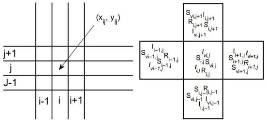
Figure 1. Spatial discretization for epidemic dynamics modeling.

Within each cell $(i,j)$, we define the following variables to describe the host and vector populations at time t:

• $S_{ij}\left(t\right)$: Population or density of susceptible hosts at $(x_{ij},y_{ij})$;
• $I_{ij}\left(t\right)$: Population or density of infected hosts at $(x_{ij},y_{ij})$;
• $R_{ij}\left(t\right)$: Population or density of recovered hosts at $(x_{ij},y_{ij})$;
• $S_{v,ij}\left(t\right)$: Population or density of susceptible vectors at $(x_{ij},y_{ij})$;
• $I_{v,ij}\left(t\right)$: Population or density of infected vectors at $(x_{ij},y_{ij})$.

Spatial interactions between cells are governed by population movement, considering the coordinates $x_{i+1,j}=x_{ij}+\delta x$ and $y_{i,j+1}=y_{ij}+\delta y$.

2.2. Balance Equations

The spatio-temporal dynamics of the populations are governed by a system of balance equations incorporating local interactions and migration fluxes between adjacent cells. We assume that only susceptible hosts can move freely, as they are healthy. The movement of infected and recovered hosts between cells is neglected. In each cell $(i,j)$, a susceptible host can only become infected through contact with an infected vector residing in the same cell. Similarly, a susceptible vector can only be infected by an infected host in the same cell. However, infected vectors are assumed to be mobile between cells.

The compartmental structure of the model within each cell is illustrated in Figure 2.

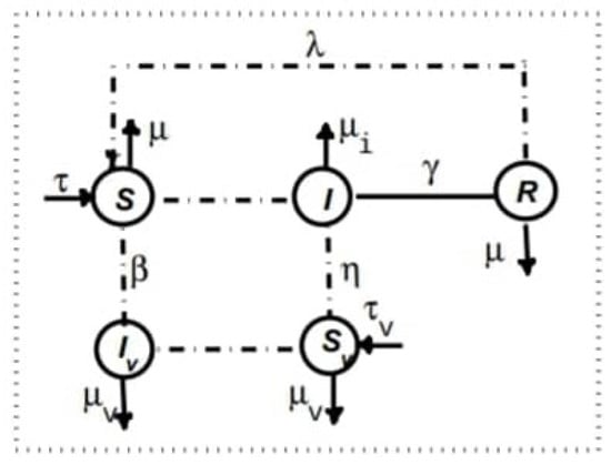
Figure 2. Compartmental scheme within a cell.

The parameters used in the model are defined as follows:

• $\tau$ and ${\tau }_v$: Growth rates of host and vector populations, respectively;
• $\beta$: Infection rate of susceptible hosts in contact with infected vectors;
• $\eta$: Infection rate of susceptible vectors in contact with infected hosts;
• $\lambda$: Rate at which recovered hosts lose immunity and become susceptible again;
• $\gamma$: Recovery rate of infected hosts;
• $\mu$, ${\mu }_i$, and ${\mu }_v$: Mortality rates of recovered hosts, infected hosts, and infected vectors, respectively.

Now, let us assume that susceptible hosts migrate to neighboring cells, while the movement of infected hosts is neglected. Let $\Omega \subset {\mathbb{R}}^2$ be the spatial domain representing the endemic area under study, and let $(x,y)\in \Omega$ and $t\ge 0$. If $\alpha$ denotes the migration rate of susceptible hosts, then over the time interval $[t,t+\delta t]$, a fraction $\alpha \delta t{S}_{ij}$ of susceptible individuals migrates to each of the four adjacent cells. Consequently, the number of susceptible individuals remaining in cell $(i,j)$ is $\delta S_{ij}-4\alpha \delta t{S}_{ij}$.

Within the same cell, the number of new infections among non-migrating hosts is given by $\delta t\beta S_{ij}(1-4\alpha )I_{v_{ij}}$. At the same time, the cell receives new susceptible hosts from neighboring cells. The balance equation for susceptible hosts becomes

$$\begin{array}{cc}\hfill S_{ij}(t+\delta t)-S_{ij}\left(t\right)& =\delta t\tau -\delta t\beta (1-4\alpha )S_{ij}{I}_{v_{ij}}\hfill \\ \hfill & +\delta t\alpha (S_{i+1,j}+S_{i-1,j}+S_{i,j-1}+S_{i,j+1})-\delta t\mu S_{ij}+\delta t\lambda R_{ij}.\hfill \end{array}$$

(1)

Assuming sufficient smoothness and using Taylor expansion, we approximate

$$S_{i+1,j}+S_{i-1,j}\approx 2S(x_{ij},y_{ij},t)+{\left(\delta x\right)}^2{\displaystyle \frac{{\partial }^{2}S}{\partial x^2}},$$

and similarly,

$$S_{i,j+1}+S_{i,j-1}\approx 2S(x_{ij},y_{ij},t)+{\left(\delta y\right)}^2{\displaystyle \frac{{\partial }^{2}S}{\partial y^2}}.$$

By setting $\delta x=\delta y$, we get:

$$S_{i+1,j}+S_{i-1,j}+S_{i,j+1}+S_{i,j-1}\approx 4S+{\left(\delta x\right)}^2\Delta S.$$

Defining $d=\alpha \times {\left(\delta x\right)}^2$ as the diffusion coefficient for susceptible hosts, we obtain the continuous model equation:

$${\displaystyle \frac{\partial S}{\partial t}}(x,y,t)=\tau -\beta (1-4\alpha )S{I}_v+(4\alpha -\mu )S+d\Delta S+\lambda R,(x,y)\in \Omega ,t\ge 0.$$

(2)

Similar derivations yield the equations for the other compartments. Letting $d_v$ denote the diffusion coefficient of the vector population, we obtain the following spatio-temporal system defined on $\Omega \times [0,+\infty )$:

$$\begin{array}{cc}\hfill {\displaystyle \frac{\partial S}{\partial t}}& =\tau -\beta (1-4\alpha )S{I}_v+(4\alpha -\mu )S+d\Delta S+\lambda R,(x,y)\in \Omega ,t\ge 0,\hfill \end{array}$$

(3)

$$\begin{array}{cc}\hfill {\displaystyle \frac{\partial I}{\partial t}}& =\beta (1-4\alpha )S{I}_v-({\mu }_i+\gamma )I,(x,y)\in \Omega ,t\ge 0,\hspace{1em}\hspace{1em}\hspace{1em}\hspace{1em}\hspace{1em}\hspace{1em} \hfill \end{array}$$

(4)

$$\begin{array}{cc}\hfill {\displaystyle \frac{\partial R}{\partial t}}& =\gamma I-(\mu +\lambda )R,(x,y)\in \Omega ,t\ge 0,\hspace{1em}\hspace{1em}\hspace{1em}\hspace{1em}\hspace{1em}\hspace{1em}\hspace{1em}\hspace{1em}\hspace{1em}\hspace{1em} \hfill \end{array}$$

(5)

$$\begin{array}{cc}\hfill {\displaystyle \hspace{1em}\frac{\partial S_v}{\partial t}}& ={\tau }_v-\eta (1-4{\alpha }_v)S_{v}I+(4{\alpha }_v-{\mu }_v)S_v+d_v\Delta S_v,(x,y)\in \Omega ,t\ge 0,\hfill \end{array}$$

(6)

$$\begin{array}{cc}\hfill {\displaystyle \frac{\partial I_v}{\partial t}}& =\eta (1-4{\alpha }_v)S_{v}I+(8{\alpha }_v-1-{\mu }_v)I_v+d_v\Delta I_v,(x,y)\in \Omega ,t\ge 0.\hfill \end{array}$$

(7)

This system describes the spatio-temporal evolution of host and vector populations during a vector-borne epidemic within the region $\Omega$.

To complete the model, boundary conditions are needed to describe interactions between the population and the environment along the domain boundary $\partial \Omega$. In vector-borne epidemics, it is commonly assumed that vectors do not migrate beyond the domain due to ecological barriers. Hence, homogeneous or inhomogeneous Neumann boundary conditions are imposed as follows:

$$\begin{array}{cc}\hfill {\displaystyle \frac{\partial S}{\partial \nu }}(x,y,t)& ={\displaystyle \frac{\partial R}{\partial \nu }}(x,y,t)=h_s(x,y,t),(x,y)\in \partial \Omega ,t\ge 0,\hfill \end{array}$$

(8)

$$\begin{array}{cc}\hfill {\displaystyle \frac{\partial I}{\partial \nu }}(x,y,t)& =h_i(x,y,t),(x,y)\in \partial \Omega ,t\ge 0,\hspace{1em}\hspace{1em}\hspace{1em}\hspace{1em}\hspace{1em}\hfill \end{array}$$

(9)

$$\begin{array}{cc}\hfill {\displaystyle \frac{\partial S_v}{\partial \nu }}(x,y,t)& ={\displaystyle \frac{\partial I_v}{\partial \nu }}(x,y,t)=0,(x,y)\in \partial \Omega ,t\ge 0,\hspace{1em}\hspace{1em}\hspace{1em}\hfill \end{array}$$

(10)

where ${\displaystyle \frac{\partial }{\partial \nu }}$ denotes the outward normal derivative on the boundary $\partial \Omega$ and where $h_s$ and $h_i$ represent boundary flux functions.

In scenarios where the boundary is closed, homogeneous Neumann boundary conditions (i.e., zero flux) are assumed for all state variables.

3. Existence, Uniqueness, and Positivity

Throughout this section, we assume that the boundary conditions for all variables are homogeneous Neumann conditions. This implies that, for the host populations, the external boundaries of the domain are considered impermeable, while for the vector populations, no outward migration is permitted due to unfavorable environmental conditions beyond their natural habitat.

3.1. Definition of Kernels and Fundamental Properties

Here, we consider the kernels as fundamental solutions (also known as Green’s functions) associated with linear parabolic partial differential operators, subject to homogeneous Neumann boundary conditions. For further mathematical background on such kernels, we refer the reader to [4,5,6].

Let $\mathcal{G}$, ${\mathcal{K}}_s$, and ${\mathcal{K}}_i$ denote the fundamental solutions associated with the following linear operators:

$${\partial }_t-d\Delta -(4\alpha -\mu ),{\partial }_t-d_v\Delta -(4{\alpha }_v-{\mu }_v),\mathrm{and}{\partial }_t-d_v\Delta -(8{\alpha }_v-1-{\mu }_v).$$

That is, these kernels satisfy

$$\begin{array}{cc}\hfill {\displaystyle \hspace{1em}\hspace{1em}\hspace{1em}\frac{\partial \mathcal{G}}{\partial t}}(x,y,t)-d\Delta \mathcal{G}(x,y,t)-(4\alpha -\mu )\mathcal{G}(x,y,t)& =\delta \left(x\right)\delta \left(y\right)\delta \left(t\right),\hfill \end{array}$$

(11)

$$\begin{array}{cc}\hfill {\displaystyle \hspace{1em}\frac{\partial {\mathcal{K}}_s}{\partial t}}(x,y,t)-d_v\Delta {\mathcal{K}}_s(x,y,t)-(4{\alpha }_v-{\mu }_v){\mathcal{K}}_s(x,y,t)& =\delta \left(x\right)\delta \left(y\right)\delta \left(t\right),\hfill \end{array}$$

(12)

$$\begin{array}{cc}\hfill {\displaystyle \frac{\partial {\mathcal{K}}_i}{\partial t}}(x,y,t)-d_v\Delta {\mathcal{K}}_i(x,y,t)-(8{\alpha }_v-1-{\mu }_v){\mathcal{K}}_i(x,y,t)& =\delta \left(x\right)\delta \left(y\right)\delta \left(t\right),\hfill \end{array}$$

(13)

for $(x,y,t)\in \Omega \times (0,\infty )$, with the homogeneous Neumann boundary conditions:

$${\displaystyle \frac{\partial \mathcal{G}}{\partial \nu }}={\displaystyle \frac{\partial {\mathcal{K}}_s}{\partial \nu }}={\displaystyle \frac{\partial {\mathcal{K}}_i}{\partial \nu }}=0\mathrm{on}\partial \Omega \times (0,\infty ),$$

(14)

where $\delta (·)$ denotes the Dirac distribution.

According to [5,6], there exists a constant $C_{\Omega }>0$, depending only on the geometry of the domain $\Omega$, such that for all $t\ge 0$

$${\parallel \mathcal{G}(·,·,t)\parallel }_{L^1(\Omega )}\le C_{\Omega },\parallel {\mathcal{K}}_s{(·,·,t)\parallel }_{L^1(\Omega )}\le C_{\Omega },{\parallel {\mathcal{K}}_i(·,·,t)\parallel }_{L^1(\Omega )}\le C_{\Omega }.$$

Integrating Equations (4) and (5) over $\Omega \times (0,t)$, and convolving Equations (3), (6), and (7) respectively with $\mathcal{G}$, ${\mathcal{K}}_s$, and ${\mathcal{K}}_i$ in the spatial variables, we use Green’s identity and the properties of the fundamental solutions to obtain the following representations (omitting explicit spatial variables $(x,y)$ for clarity):

$$\begin{array}{c}{\displaystyle S\left(t\right)=(S_0\ast \mathcal{G})\left(t\right)+{\int }_0^t{\int }_{\Omega }\mathcal{G}(x-\xi ,y-\zeta ,t-s)\left[\tau -\beta (1-4\alpha )S(\xi ,\zeta ,s)I_v(\xi ,\zeta ,s)\right.}\\ \left.+\lambda R(\xi ,\zeta ,s)\right]d\xi d\zeta ds,\end{array}$$

(15)

$${\displaystyle I\left(t\right)=I_0+{\int }_0^t\left[\beta (1-4\alpha )S\left(s\right)I_v\left(s\right)-({\mu }_i+\gamma )I\left(s\right)\right]ds}$$

(16)

$${\displaystyle R\left(t\right)=R_0+{\int }_0^t\left[\gamma I\left(s\right)-(\mu +\lambda )R\left(s\right)\right]ds}$$

(17)

$$\begin{array}{c}{\displaystyle S_v\left(t\right)=(S_{v,0}\ast {\mathcal{K}}_s)\left(t\right)+{\int }_0^t{\int }_{\Omega }{\mathcal{K}}_s(x-\xi ,y-\zeta ,t-s)\left[{\tau }_v-\eta (1-4{\alpha }_v)\right.}\\ \left.\times S_v(\xi ,\zeta ,s)I(\xi ,\zeta ,s)\right]d\xi d\zeta ds,\end{array}$$

(18)

$$\begin{array}{c}{I}_v\left(t\right)=(I_{v,0}\ast {\mathcal{K}}_i)\left(t\right)+{\int }_0^t{\int }_{\Omega }{\mathcal{K}}_i(x-\xi ,y-\zeta ,t-s)\left[\eta (1-4{\alpha }_v)S_v(\xi ,\zeta ,s)I(\xi ,\zeta ,s)\right]d\xi d\zeta ds.\end{array}$$

(19)

Here, $(f\ast K)\left(t\right)$ denotes the spatial convolution of the initial data with the corresponding kernel, i.e.,

$$(f\ast K)\left(t\right)(x,y)={\int }_{\Omega }K(x-\xi ,y-\zeta ,t)f(\xi ,\zeta )d\xi d\zeta .$$

A weak solution of the model is then defined as a vector-valued function $Z=\left(S,I,R,S_v,I_v\right)$ that satisfies the above integral equations for all $(x,y,t)\in \Omega \times [0,\infty )$.

3.2. Existence and Uniqueness of a Weak Solution

The following result is established:

Theorem 1 

(Existence and uniqueness of a weak solution). For any initial data $(S_0,I_0,R_0,S_{0,v},$$I_{0,v})\in {\left(L^{\infty }(\Omega )\right)}^5$, there exists a unique global weak solution in time: $\left(S,I,R,S_v,I_v\right)\in {\left(L^{\infty }({\mathbb{R}}_{+},L^{\infty }(\Omega ))\right)}^5$ to the problem (3)–(7) with homogeneous Neumann boundary conditions.

Proof. 

We employ the Banach fixed-point theorem to prove existence and uniqueness. We define the Banach space:

$${\mathcal{X}}_T:=\left\{Z=(S,I,R,S_v,I_v)\in {\left(C([0,T];L^{\infty }(\Omega ))\right)}^5|{\displaystyle \frac{\partial u}{\partial \nu }}=0\mathrm{on}\partial \Omega \mathrm{for}\mathrm{each}\mathrm{component}u\mathrm{of}Z\right\}$$

for fixed small time $T>0$. Equip ${\mathcal{X}}_T$ with the norm

$${\parallel Z\parallel }_{{\mathcal{X}}_T}:=\underset{u\in \{S,I,R,S_v,I_v\}}{max}{\parallel u\parallel }_{L^{\infty }([0,T]\times \Omega )}.$$

Define the operator $\Phi$ by

$$\Phi \left(Z\right):=\left(\begin{array}{c}{\displaystyle (S_0\ast \mathcal{G})\left(t\right)+{\int }_0^t\mathcal{G}(t-s)\ast \left[\tau -\beta (1-4\alpha )S\left(s\right)I_v\left(s\right)+\lambda R\left(s\right)\right]ds}\\ {\displaystyle I_0+{\int }_0^t\left[\beta (1-4\alpha )S\left(s\right)I_v\left(s\right)-({\mu }_i+\gamma )I\left(s\right)\right]ds}\\ {\displaystyle R_0+{\int }_0^t\left[\gamma I\left(s\right)-(\mu +\lambda )R\left(s\right)\right]ds}\\ {\displaystyle (S_{v,0}\ast {\mathcal{K}}_s)\left(t\right)+{\int }_0^t{\mathcal{K}}_s(t-s)\ast \left[{\tau }_v-\eta (1-4{\alpha }_v)S_v\left(s\right)I\left(s\right)\right]ds}\\ {\displaystyle (I_{v,0}\ast {\mathcal{K}}_i)\left(t\right)+{\int }_0^t{\mathcal{K}}_i(t-s)\ast \left[\eta (1-4{\alpha }_v)S_v\left(s\right)I\left(s\right)\right]ds}\end{array}\right),$$

where all convolutions are in the spatial variables.

We can observe that the operator $\Phi$ maps every element Z of ${\mathcal{X}}_T$ into an element of ${\mathcal{X}}_T$. Indeed, since the kernels $\mathcal{G}$, ${\mathcal{K}}_s$, and ${\mathcal{K}}_i$ satisfy the Neumann boundary conditions, and the initial data are compatible, their convolutions with bounded functions also satisfy the boundary conditions. Therefore, $\Phi \left(Z\right)\in {\mathcal{X}}_T$ for all $Z\in {\mathcal{X}}_T$.

-

Since $\mathcal{G},{\mathcal{K}}_s,{\mathcal{K}}_i$ are in $L^1(\Omega )$ uniformly in t (by [5,6]), and the initial data are bounded, we have

$$\parallel S_0{\ast \mathcal{G}\left(t\right)\parallel }_{L^{\infty }(\Omega )}\le \parallel S_0{\parallel }_{L^{\infty }}·{\parallel \mathcal{G}\left(t\right)\parallel }_{L^1}\le M{C}_{\Omega }.$$

Similarly for $S_{v,0}$ and $I_{v,0}$.

-

For the integral terms, we use the Young convolution inequality:

$${\parallel \mathcal{G}(t-s)\ast f\left(s\right)\parallel }_{L^{\infty }(\Omega )}\le {\parallel f\left(s\right)\parallel }_{L^{\infty }(\Omega )}·{\parallel \mathcal{G}(t-s)\parallel }_{L^1(\Omega )}\le C_{\Omega }{\parallel f\left(s\right)\parallel }_{L^{\infty }(\Omega )}.$$

Applying this to all source terms, and using the assumption that $Z\in {\mathcal{X}}_T$ with ${\parallel Z\parallel }_{{\mathcal{X}}_T}\le M$, we get

$${\parallel \Phi \left(Z\right)\parallel }_{{\mathcal{X}}_T}\le C_1+C_{2}T{M}^2,$$

for constants $C_1$, $C_2$ depending on model parameters and $C_{\Omega }$.

Let $Z_1=(S_1,I_1,\dots )$ and $Z_2=(S_2,I_2,\dots )\in {\mathcal{X}}_T$. Consider the difference ${\Phi }_S\left(Z_1\right)-{\Phi }_S\left(Z_2\right)$ in the susceptible host component. Using the bilinearity of the product, we decompose

$$S_1{I}_{v1}-S_2{I}_{v2}=(S_1-S_2)I_{v1}+S_2(I_{v1}-I_{v2}).$$

We estimate

$$\begin{array}{ccc}\hfill {∥{\Phi }_S\left(Z_1\right)-{\Phi }_S\left(Z_2\right)∥}_{\infty }& \le & {\displaystyle {\int }_0^t∥\mathcal{G}(t-s)\ast \left[\beta (1-4\alpha )((S_1-S_2)I_{v1}+S_2(I_{v1}-I_{v2}))+\right.}\hfill \\ & & {\left.\lambda (R_1-R_2)\right]∥}_{\infty }ds\hfill \\ & \le & {\displaystyle C_{\Omega }{\int }_0^T{∥\beta (1-4\alpha )((S_1-S_2)I_{v1}+S_2(I_{v1}-I_{v2}))+\lambda (R_1-R_2)∥}_{\infty }}\hfill \\ & \le & CT\left(\parallel S_1-S_2{\parallel }_{\infty }\parallel I_{v1}{\parallel }_{\infty }+\parallel S_2{\parallel }_{\infty }\parallel I_{v1}-I_{v2}{\parallel }_{\infty }+{\parallel R_1-R_2\parallel }_{\infty }\right)\hfill \end{array}$$

where C is the constant depending of the domain and the parameters. Since both $I_{v1}$ and $S_2$ are bounded by $M$, we finally obtain

$$\parallel {\Phi }_S\left(Z_1\right)-{\Phi }_S\left(Z_2\right){\parallel }_{\infty }\le CTmax\{M,1\}\left(\parallel S_1-S_2{\parallel }_{\infty }+\parallel I_{v1}-I_{v2}{\parallel }_{\infty }+{\parallel R_1-R_2\parallel }_{\infty }\right).$$

The same method applies to all other components, leading to

$$\parallel \Phi \left(Z_1\right)-\Phi \left(Z_2\right){\parallel }_{X_T}\le CTmax\{M,1\}{\parallel Z_1-Z_2\parallel }_{X_T},$$

which yields the contraction property for sufficiently small T. Hence, by the Banach fixed-point theorem, there exists a unique fixed point $Z\in {\mathcal{X}}_T$, i.e., a unique local weak solution.

Let us now establish the global existence. Since the $L^{\infty }$ norm is preserved and no blow-up occurs (all source terms are polynomial and Lipschitz on bounded sets), the solution can be extended step by step to any finite time. Therefore, the solution exists globally in time and remains in $L^{\infty }$. □

3.3. Existence of a Positive Classical Solution

We now demonstrate that the obtained solutions are also positive. To achieve this, we recall the following general theorem concerning reaction–diffusion systems.

Consider the following reaction–diffusion system:

$$\left\{\begin{array}{cc}{\partial }_t{u}_i-{\Lambda }_i{u}_i=f_i(u_1,\dots ,u_m)\hfill & \mathrm{in}(0,T)\times \Omega ,\hfill \\ {\displaystyle \frac{\partial u_i}{\partial n}}=0\hfill & \mathrm{on}(0,T)\times \partial \Omega ,\hfill \\ u_i(0,·)=u_{i0}\hfill & \mathrm{in}\Omega ,\hfill \end{array}\right.$$

(20)

for $i=1,\dots ,m$, where

• $\Omega$ is a bounded domain in ${\mathbb{R}}^N$ with a smooth boundary $\partial \Omega$,
• ${\Lambda }_i>0$ are the diffusion coefficients,
• $u_{i0}\in L^{\infty }(\Omega )$ are the initial conditions, assumed to be non-negative, i.e., $u_{i0}\ge 0$,
• The functions $f_i:{\mathbb{R}}^m\to \mathbb{R}$ represent the reaction terms and are assumed to be of class $C^1$.

We impose the quasi-positivity condition on $f_i$, which ensures that the solutions remain non-negative:

$$f_i(u_1,\dots ,u_{i-1},0,u_{i+1},\dots ,u_m)\ge 0,\mathrm{for}\mathrm{all}u\in {[0,+\infty )}^m,i=1,\dots ,m.$$

(21)

The following theorem holds

Theorem 2. 

Under the above assumptions, for any initial data $u_{i0}\in L^{\infty }(\Omega )$ with $u_{i0}\ge 0$, there exists a unique global solution

$$u=(u_1,\dots ,u_m)\in {\left(L^{\infty }((0,T)\times \Omega )\right)}^m,\forall T>0.$$

Moreover, this solution is non-negative, i.e., $u_i(t,x)\ge 0,\forall t\ge 0,\forall x\in \Omega .$ Finally, if the functions $f_i$ are of class ${\mathcal{C}}^2$, then the solution to the problem is also regular, i.e., $u_i\in {\mathcal{C}}^2\left([0,T]\times \overline{\Omega }\right).$

Proof. 

The proof relies on the results of Michel Pierre concerning the global existence of solutions for reaction–diffusion systems under assumptions of quasi-positivity and total mass control. Indeed, Michel Pierre’s work shows that, under these assumptions, system (20) admits global solutions in time that remain bounded and non-negative. For more details, one can refer to Michel Pierre [7], as well as [8,9,10] for further developments. □

Applying this result to our studied system, we establish the following theorem:

Theorem 3. 

Assume that the diffusion coefficients satisfy $d>0$ and $d_v>0$. If the model parameters satisfy the following positivity conditions,

$$\left\{\begin{array}{ccc}\hfill 1-4\alpha & >& 0,\hfill \\ \hfill 1-4{\alpha }_v& >& 0,\hfill \end{array}\right.$$

(22)

then, for any positive initial data, $\left(S_0,I_0,R_0,S_{0,v},I_{0,v}\right)\ge 0\mathrm{in}{\left(L^{\infty }(\Omega )\right)}^5,$ there exists a unique positive classical solution $\left(S,I,R,S_v,I_v\right)\in {\left({\mathcal{C}}^2\left([0,T]\times \overline{\Omega }\right)\right)}^5$ to the system (3)–(7), for all $T>0$.

Proof. 

The key idea is to reformulate the system (3)–(7) in the general form of the reaction–diffusion system (20).

• Identification of the reaction terms: It is straightforward to verify that the source term of our system satisfies the quasi-positivity condition due to (22).
• Regularity of the terms: The right-hand side of the system is of class ${\mathcal{C}}^2$, which ensures that the obtained solutions are also regular.
• Application of the global existence theorem: By applying Theorem 2, we immediately conclude that there exists a unique classical solution

  $$\left(S,I,R,S_v,I_v\right)\in {\left({\mathcal{C}}^2\left([0,T]\times \overline{\Omega }\right)\right)}^5.$$

• Furthermore, this solution is positive for any positive initial data, ensuring the epidemiological consistency of the model. □

Thus, we have established the existence and uniqueness of classical and positive solutions for our epidemiological system, under appropriate positivity conditions on the model parameters. This result directly follows from global existence theorems for reaction–diffusion systems and ensures the mathematical validity of the studied model.

4. Qualitative Analysis of the Model

In this section, we compute the basic reproduction number ${\mathcal{R}}_0$ using the Next Generation Matrix (NGM) method introduced by Diekmann et al. [11] and rigorously developed in the framework of Shuai and van den Driessche [12,13]. We also verify that all required conditions for the application of their global stability theorem are satisfied in our setting.

4.1. Model Reduction and Infection Subsystem

We first isolate the infection subsystem by identifying the infected compartments: the infected hosts I and infected vectors $I_v$. The state vector of the infected subsystem is defined as $\mathbf{x}={(I,I_v)}^{\top }$. The nonlinear infection system can be written as

$${\displaystyle \frac{d\mathbf{x}}{dt}}=\mathcal{F}\left(\mathbf{x}\right)-\mathcal{V}\left(\mathbf{x}\right),$$

(23)

where $\mathcal{F}\left(\mathbf{x}\right)$ represents the rate of new infections, and $\mathcal{V}\left(\mathbf{x}\right)$ captures the transfer of individuals out of the infected compartments (by recovery, death, etc.).

We define

$$\mathcal{F}\left(\mathbf{x}\right)=\left(\begin{array}{c}\beta (1-4\alpha )S{I}_v\\ \eta (1-4{\alpha }_v)S_{v}I\end{array}\right),\mathcal{V}\left(\mathbf{x}\right)=\left(\begin{array}{c}({\mu }_i+\gamma )I\\ (1+{\mu }_v-8{\alpha }_v)I_v\end{array}\right).$$

(24)

4.2. Linearization at the Disease-Free Equilibrium

Let $(S_0,I_0,R_0,S_{v,0},I_{v,0})$ be the disease-free equilibrium (DFE) of the system. Assuming $I_0=I_{v,0}=0$, the DFE is given by

$$(S_0,R_0,S_{v,0})=\left({\displaystyle \frac{\tau }{\mu }},0,{\displaystyle \frac{{\tau }_v}{{\mu }_v}}\right).$$

The Jacobian matrices of $\mathcal{F}$ and $\mathcal{V}$ evaluated at the DFE are given by

$$\begin{array}{cc}\hfill \hspace{1em}\hspace{1em}\hspace{1em}F& ={\left.{\displaystyle \frac{\partial \mathcal{F}}{\partial \mathbf{x}}}\right|}_{\mathrm{DFE}}=\left(\begin{array}{cc}0& \beta (1-4\alpha )S_0\\ \eta (1-4{\alpha }_v)S_{v,0}& 0\end{array}\right),\hfill \end{array}$$

(25)

$$\begin{array}{cc}\hfill V& ={\left.{\displaystyle \frac{\partial \mathcal{V}}{\partial \mathbf{x}}}\right|}_{\mathrm{DFE}}=\left(\begin{array}{cc}{\mu }_i+\gamma & 0\\ 0& 1+{\mu }_v-8{\alpha }_v\end{array}\right).\hfill \end{array}$$

(26)

4.3. Computation of the Basic Reproduction Number

The next generation matrix is defined by $K=F{V}^{-1}$, hence

$$K=\left(\begin{array}{cc}0& {\displaystyle \frac{\beta (1-4\alpha )S_0}{1+{\mu }_v-8{\alpha }_v}}\\ {\displaystyle \frac{\eta (1-4{\alpha }_v)S_{v,0}}{{\mu }_i+\gamma }}& 0\end{array}\right).$$

(27)

The basic reproduction number is the spectral radius of K:

$${\mathcal{R}}_0=\rho \left(K\right)=\sqrt{{\displaystyle \frac{\beta (1-4\alpha )S_0}{1+{\mu }_v-8{\alpha }_v}}·{\displaystyle \frac{\eta (1-4{\alpha }_v)S_{v,0}}{{\mu }_i+\gamma }}}.$$

(28)

4.4. Verification of Shuai-Van Den Driessche Conditions

The application of the global stability theorem in [12] requires the following conditions:

(C1)

The DFE is globally asymptotically stable for the infection-free subsystem (i.e., when $I=I_v=0$). This holds in our model since all equations without infections are linear and exponentially stable.

(C2)

The infection subsystem can be written as ${\displaystyle \frac{d\mathbf{x}}{dt}}=\mathcal{F}(\mathbf{x},\mathbf{y})-\mathcal{V}\left(\mathbf{x}\right)$ where $\mathcal{F}$ is non-negative when $\mathbf{x}\ge 0$ and $\mathcal{V}$ is an M-matrix (i.e., diagonally dominant with non-positive off-diagonal entries). This is satisfied since

$$\mathcal{F}\left(\mathbf{x}\right)\ge 0,\mathrm{and}\mathcal{V}\left(\mathbf{x}\right)=D\mathbf{x},\mathrm{with}D=diag({\mu }_i+\gamma ,1+{\mu }_v-8{\alpha }_v).$$

(C3)

$\mathcal{F}(\mathbf{x},\mathbf{y})$ is $C^1$ in both arguments and $\mathcal{F}(0,\mathbf{y})=0$. This is clear from the definition.

(C4)

The matrix V is non-singular with positive diagonal entries. This follows from the assumption $1+{\mu }_v-8{\alpha }_v>0$ and the biological positivity of the other parameters.

Hence, all conditions of the theorem from Shuai and van den Driessche [12] are satisfied, allowing us to conclude that

• If ${\mathcal{R}}_0<1$, then the DFE is globally asymptotically stable.
• If ${\mathcal{R}}_0>1$, then the infection can persist, and the DFE is unstable.

5. Conclusions

In this study, we developed a spatio-temporal mathematical model to describe the spread of vector-borne diseases, incorporating population dynamics and the spatio-temporal factors that influence pathogen transmission. We conducted a theoretical analysis of the system, demonstrating the existence, uniqueness, and positivity of solutions. Additionally, we investigated key epidemiological parameters, including the basic reproduction number ${\mathcal{R}}_0.$ Our study provides a result about the spread of epidemics when the ${\mathcal{R}}_0$ is greater than one.

References

- Jorge, D.; Oliveira, J.; Miranda, J.; Andrade, R.; Pinho, S. Estimating the effective reproduction number for heterogeneous models using incidence data. R. Soc. Open Sci. 2022, 9, 220005. [Google Scholar] [CrossRef] [PubMed]
- Mantha, S. Basic reproduction number, effective reproduction number and herd Immunity: Relevance to opening up of economies hampered by COVID-19. J. Allergy Infect. Dis. 2020, 1, 32–34. [Google Scholar]
- Osei-Buabeng, V.; Frimpong, A.A.; Barnes, B. Mathematical modelling of the epidemiology of Corona Virus Infection with constant spatial diffusion term in Ghana. Comput. Methods Differ. Equ. 2024, 13, 870–884. [Google Scholar]
- Evans, L.C. Partial Differential Equations, 2nd ed.; American Mathematical Society: Providence, RI, USA, 2022. [Google Scholar]
- Ouhabaz, E. Analysis of Heat Equations on Domains; London Mathematical Society Monographs Series; Princeton University Press: Princeton, NJ, USA, 2005. [Google Scholar]
- Pazy, A. Semigroups of Linear Operators and Applications to Partial Differential Equations; Springer: Cham, Switzerland, 1983. [Google Scholar]
- Pierre, M. Global existence in reaction-diffusion systems with control of mass: A survey. Milan J. Math. 2010, 78, 417–455. [Google Scholar] [CrossRef]
- Amann, H. Global existence for semilinear parabolic problems. J. Reine Angew. Math. 1985, 360, 47–83. [Google Scholar]
- Pierre, M.; Schmitt, D. Blow up in reaction-diffusion systems with dissipation of mass. SIAM J. Math. Anal. 1997, 28, 259–269. [Google Scholar] [CrossRef]
- Pierre, M.; Schmitt, D. Global existence for a reaction-diffusion system with a balance law. In Semigroups of Nonlinear Operators and Applications, Proceedings of the Curaçao Conference, August 1992; Goldstein, G.R., Goldstein, G.A., Eds.; Springer: Dordrecht, The Netherlands, 1993. [Google Scholar]
- Van Den Driessche, P. Reproduction numbers of infectious disease models. Infect. Dis. Model. 2017, 2, 288–303. [Google Scholar] [CrossRef] [PubMed]
- Shuai, Z.; Van Den Driessche, P. Global stability of infectious disease models using Lyapunov functions. SIAM J. Appl. Math. 2013, 73, 1513–1532. [Google Scholar] [CrossRef]
- Van Den Driessche, P.; Watmough, J. Further notes on the basic reproduction number. In Mathematical Epidemiology; Springer: Berlin/Heidelberg, Gernamy, 2008. [Google Scholar]
Disclaimer/Publisher’s Note: The statements, opinions and data contained in all publications are solely those of the individual author(s) and contributor(s) and not of MDPI and/or the editor(s). MDPI and/or the editor(s) disclaim responsibility for any injury to people or property resulting from any ideas, methods, instructions or products referred to in the content. |
© 2025 by the authors. Licensee MDPI, Basel, Switzerland. This article is an open access article distributed under the terms and conditions of the Creative Commons Attribution (CC BY) license (https://creativecommons.org/licenses/by/4.0/).