Abstract
We show how the dynamics of inflation as represented by the Phillips curve follow from a response formalism suggested by Phillips and motivated by the Keynesian notion that it takes time for an economy to respond to an economic shock. The resulting expressions for the Phillips curve are isomorphic to those of anelasticity—a result that provides a straightforward and parsimonious approach to macroeconomic-model construction. Our approach unifies forms of the Phillips curve that are used to account for time dependence of the Phillips curve, expands the possible microeconomic explanations of this time dependence, and broadens the reach of this formalism in economics.
JEL Classification:
E24; E31; E32; E71; J30
1. Introduction
The dependence of wage inflation on the unemployment rate—a relationship known as the Phillips curve—was developed originally by Phillips as part of his research program concerning macroeconomic stability and control [1,2,3,4], and subsequently evolved into a relationship between general price inflation and unemployment [5] that plays a central role in macroeconomic policy development in government and academia [6,7,8,9,10,11,12,13,14,15,16,17,18]. Observed deviations of this dependence from commonly used forms of the Phillips curve, including whether the curve is linear or nonlinear, changes in the slope, and time-varying applicability of a particular specifications, however, have led to questions concerning this relationship in general and to whether the Phillips curve has broken down in particular [6,15,19,20,21,22,23]. Given the importance of the Phillips curve in macroeconomic policy development [8,9,10,11,15,17], a reconciliation of these seemingly contradictory assessments is warranted, and a goal of this paper is to show that a time-dependent extension of the Phillips curve that treats deviations from the Phillips curve known as Phillips loops reconciles these observations in a parsimonious and empirically sound manner.
Phillips loops are deviations from the Phillips curve associated with business cycles: inflation being greater than that indicated by the Phillips curve during economic expansions when unemployment is decreasing and inflation is increasing, and less than that given by the Phillips curve when unemployment is increasing and inflation is decreasing. These loops, commented on at length by Phillips [3], have been and remain a subject of interest to both academics [24,25,26,27,28,29,30,31,32,33,34] and central banks [35,36,37,38], and imply that time is a critical component of the unemployment–inflation relationship. And, while time dependence has been incorporated into the Phillips curve in earlier work, this has largely been a consequence of the expectations models that have been employed in what have come to be known as the New Keynesian Phillips curve models [39,40,41]; models have come under recent criticism [10,11,15].
In this paper, we build on Phillips’ work by noting that the formal assumptions underlying the Phillips curve and Phillips loops are identical to the assumptions underlying a variety of relaxation processes in condensed-matter physics including magnetic, dielectric, and anelastic relaxation [42,43]. These physical phenomena all involve time-dependent relaxation toward newly established equilibria that follow from a change in a driving force. Since these physical phenomena share a common mathematical description of relaxation/response and since these physical phenomena and inflation dynamics share a number of underlying assumptions, we make the ansatz that these phenomena all share a common mathematical description. This approach has—based on similar reasoning—also proved successful in modeling other economic phenomena [44,45], further recommending this line of inquiry.
The theory of anelasticity provides a useful framework with which to develop our treatment of the Phillips curve because of the similarity between some of the equations that have appeared in the Phillips-curve literature and the scalar representation of anelasticity. Consequently, we continue below in Section 2 with an anelastic analysis of Phillips loops using Phillips’ original curve and data from the United Kingdom. We extend this analysis to the common linear version of the Phillips curve in Section 3 with an assessment of the Phillips curve in the United States and Canada in the mid-20th century, and show that the anelastic approach unifies these analysis with early work on inflation dynamics by Fisher. We develop a source of the time dependence of the Phillips curve in terms of decision dynamics in Section 4 and close in Section 5 with a discussion and summary.
2. The Original Phillips Curve and Loops
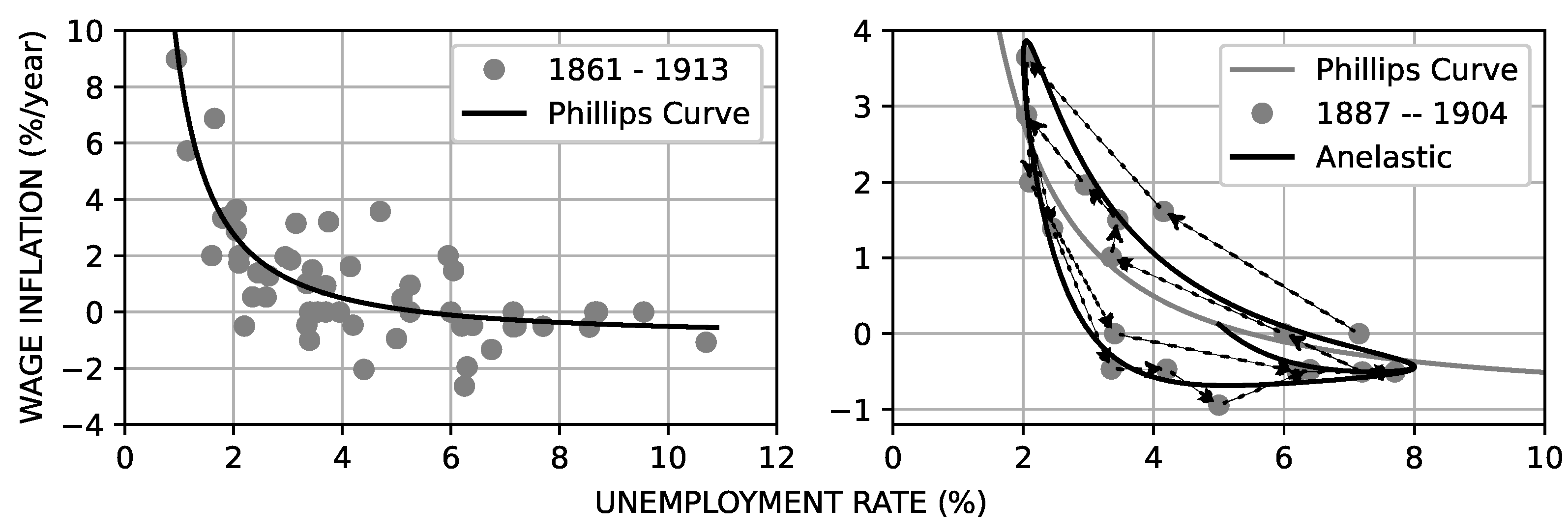
The original Phillips curve, shown together with the data from which it was obtained in the left-hand panel Figure 1, was observed by Phillips to illustrate an example of supply and demand:
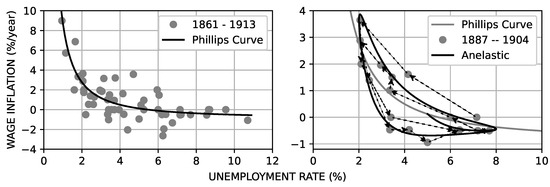
Figure 1.
The original Phillips curve together with the data used to fit it (left-hand panel). The 1887–1904 subset of Phillips data, together with the original Phillips curve and the anelastic model of the Phillips loop (right-hand panel). The length of each arrow in the left-hand panel is one year. The data are from Table 1 of reference [46].
“When the demand for labour is high and there are very few unemployed we should expect employers to bid wage rates up quite rapidly, each firm and each industry being continually tempted to offer a little above the prevailing rates to attract the most suitable labour from other firms and industries. On the other hand it appears that workers are reluctant to offer their services at less than the prevailing rates when the demand for labour is low and unemployment is high so that wage rates fall only very slowly. The relation between unemployment and the rate of change of wage rates is therefore likely to be highly nonlinear.”(p. 283, [3])
The expression Phillips used to express wage inflation, , as a function of the unemployment rate, u, is [3]
with constants , , and , and is shown by the solid curve in both panels of Figure 1. In keeping with the notation of Phillips, the additional term often included in the econometric literature to indicate the presence of other economic shocks is not present in this or other expressions of the Phillips curve that we develop below. These shocks are, however, understood to be present when analyzing data.
While it is tempting to see the scatter of the data about the Phillips curve as the result of random shocks to the economy, there is structure to the departures from the Phillips curve as shown in the right-hand panel of Figure 1. In this panel, the data are connected by arrows to indicate their temporal ordering, and two counterclockwise loops are seen. These loops are shown in Figures 2–8 of Phillips’ paper and discussed by Phillips at some length, first conceptually
“It seems possible that a second factor influencing the rate of change of money wage rates might be the rate of change of the demand for labour, and so of unemployment. Thus in a year of rising business activity, with the demand for labour increasing and the percentage unemployment decreasing, employers will be bidding more vigorously for the services of labour than they would be in a year during which the average percentage unemployment was the same but the demand for labour was not increasing. Conversely in a year of falling business activity, with the demand for labour decreasing and the percentage unemployment increasing, employers will be less inclined to grant wage increases, and workers will be in a weaker position to press for them, than they would be in a year during which the average percentage unemployment was the same but the demand for labour was not decreasing.”(p. 283, [3])
- and later theoretically with his suggestion of enhancing Equation (1) with a time-derivative term to model the loops (footnote 3, [3]). The use of time-derivatives was not explored further by Phillips in this paper due to issues of computational complexity.
To develop Phillips’ suggestion concerning the modelling of Phillips loops, we begin by rewriting Equation (1) as a nonlinear version of Hooke’s law shifted by the constant a
where
and noting that the Phillips curve embodies the three postulates—with postulate 2 modified for nonlinearity—that Nowick and Berry identified for elasticity: (i) for every level of the unemployment rate there is a unique level of the inflation rate (and vice versa), (ii) the relationship between the unemployment rate and the inflation rate is nonlinear, and (iii) the new level of the inflation rate that follows from a change in the unemployment rate is established immediately [42].
Anelasticity follows from elasticity by relaxing the third postulate to allow for the passage of time between a change in the unemployment rate and the realization of the new equilibrium inflation rate, and to this end we applied the nonlinear anelasticity approach of Wuttig and Suzuki [47] to the Phillips curve that yields
where is the relaxation time and where the functions and correspond to the relaxed (i.e., equilibrium) and unrelaxed (i.e., disequilibrium immediately following a change in the unemployment rate) responses of the economy, respectively. Phillips argued that a time-dependent unemployment term is needed to explain the deviation of inflation from Equation (1) for a given level of unemployment. An identical, symmetric, case can be made for explaining the deviation of unemployment from Equation (1) for a given level of inflation, and suggests the functional form given in Equation (4).
Operationally, the anelastic approach separates the instantaneous proportionality given in Equation (2) into two components: that represents the inflation change that occurs instantaneously on the time scale of data measurement (e.g., monthly or quarterly) and that represents the equilibrium extent of the inflation response to a change in the unemployment rate. The transition between the instantaneous response () and the equilibrium response () is, as we shall see below, a time-dependent process governed by the rate constant .
The ability of the anelastic form of the Phillips curve (Equation (4)) to provide a representation of the Phillips loops is shown by the solution of Equation (4) in the right-hand panel of Figure 1 for an idealized business cycle given by with parameters, , , , , , and . With this expression for Equation (4) becomes a simpler ODE which can be solved numerically; in our case using odeint. This solution clearly tracks the general trajectory of the Phillips loops in this economy, with further deviations attributable to other economic shocks.
3. The Linear Phillips Curve and Loops
Despite the nonlinear nature of the original Phillips curve, subsequent work has focused largely on a linear (also known as reduced-form) approximation of this relationship. This form of the Phillips curve follows from the replacements , , and . With these replacements the linear Phillips curve becomes
with the associated anelastic form
As in the nonlinear case discussed above, the proportionality term J has been divided into the instantaneous component and the relaxed component , the constant governs the rate of relaxation in response to a shock, and the steady-state is given by . If we assume that the central bank targets a rate of inflation, , that is consistent with the natural rate of unemployment, , with associated equilibrium expression , and identify the terms involving derivatives with expected inflation, or where the dots denote time derivatives, then the linear anelastic form of the Phillips curve can be written as
which is the standard forward-looking, expectations-augmented Phillips curve. [11]
The Phillips loops associated with the linear Phillips curve are solutions to Equation (6) as illustrated in Figure 2 where we see the response of inflation to an idealized business cycle given by a sinusoidal unemployment gap, ( being the unemployment rate about which the business cycle oscillates), given by
where and is the cyclic frequency of the business cycle.
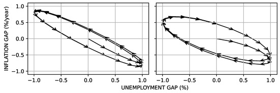
Figure 2.
The response of inflation to a cyclic unemployment gap. The arrows indicate the temporal ordering of the solutions. The parameters for the left-hand panel are , and years; those of the right-hand panel are , and years. The length of each arrow is one quarter of a year and the period of the business cycle is 5 years.
Inflation moves relative to the unemployment gap in a manner determined by the loss angle
where , being the level of inflation about which the business cycle oscillates, and where is related to the cyclic frequency of the business cycle by [42,48]
Since the loss angle is an indication of the internal friction in an anelastic system [42,48], it provides a quantitative measurement of economic friction in the unemployment–inflation relationship.
The Phillips loop shown in the left-hand panel of Figure 2 is the solution to Equation (6) beginning with the economy in equilibrium; the inflation gap and the unemployment gap are equal to zero. After an initial transient the economy settles into a Phillips loop with a counterclockwise rotation: the arrows indicate the direction of rotation of the economy, and each arrow has a length of one quarter of a year. Comparing this panel with the panel for the United Kingdom in Figure 1, we see that the linear anelastic Phillips curve can generate loops with the same direction of rotation. In the right-hand panel of Figure 2 we see a similar simulation with , resulting in a clockwise rotation that we will see in the United States and Canada below.
Commonly encountered discrete forms of the anelastic Phillips curve—also known as partial-adjustment models—follow from discretizing Equation (6). For example, the forward-difference Euler discretization yields
and when , this becomes
which is identical in structure to one of the Phillips curves used by the Congressional Budget Office (CBO) [12]. Further lags can be generated using higher-order discretization schemes. For example, a Phillips curve with n lags of inflation and unemployment follows directly from an n-step Adams–Bashforth discretization of the anelastic Phillips curve. The Phillips curve with four (4) lags used by the CBO [12,16] has a functional form similar to that of a 4-step Adams–Bashforth discretization of Equation (6). These anelastic Phillips curves differ, however, from the partial adjustment models that have appeared in the literature in two important ways: the number of free parameters is determined by the differential equation relating unemployment and inflation (i.e., the number of coefficients in Equation (6)), while the number of lagged terms is determined independently by the chosen order of the discretization. For example, while the Phillips curve used by the CBO has eight parameters—one for each of the four lags of inflation and unemployment—the anelastic Phillips curve based on a 4-step Adams–Bashforth discretization of Equation (6) has only three parameters (, and ) with the coefficients of lagged inflation and unemployment being functions of these parameters. Thus, the anelastic approach provides a convenient way to avoid overspecifying the relationship between inflation and unemployment while simultaneously providing the lag flexibility needed to represent the data.
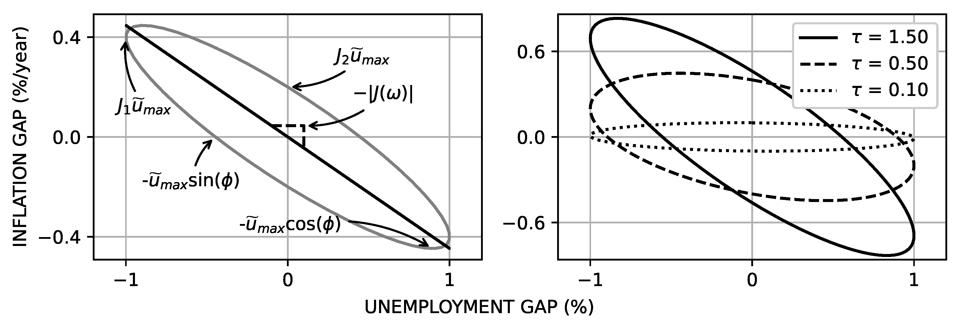
A useful addition to the regression analysis discussed above follows from the identification by Gittings [35] of the steady-state Phillips loop as a Lissajous ellipse as shown in Figure 3.
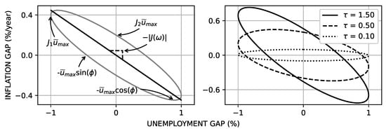
Figure 3.
The Phillips loop as a Lissajous ellipse. The parameters for the left-hand panel are the same as those of Figure 2: , and years. The parameters for the right-hand panel are and , with in years as indicated. The left-hand panel was adapted from Figure 3.3 of reference [48].
The loops in this figure were generated using with , resulting in a response of [48], the loss angle being given by Equation (10). The magnitude of the slope of the Phillips curve corresponding to the major axis of the Phillips loop show as the solid black line in the left-hand panel of Figure 3 is given by [48]
The magnitude of this slope lies between and , and would be the magnitude of the slope of the Phillips curve expected from a typical regression analysis using Equation (5) of data generated by Equation (6). In the right-hand panel of Figure 3 we see that this approach provides a framework for explaining recently observed flattening of the Phillips curve (cf. reference [17] and references therein), as well as addressing the existence of a long-term tradeoff between unemployment and inflation that we discuss below in Section 5.
Examples of Phillips loops from the United States and Canada are shown in Figure 4.
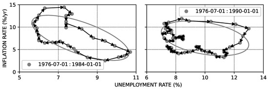
Figure 4.
Inflation as a function of the unemployment rate in the United States (left-hand panel) and Canada (right-hand panel). The length of each arrow is three months. The associated Lissajous ellipses are shown in grey. In the left-hand panel of Figure 4 the inflation rate is the annual percent change in the consumer price index (CPI) and the unemployment rate is the reported annual unemployment rate. These time series with identifiers CPIAUCSL, and UNRATE, respectively, were obtained from the Federal Reserve Economic Database (FRED). The inflation and unemployment rate time series for Canada shown in the right hand panel of Figure 4 were obtained from the quarterly CPGRLE01CAM659N and LRUNTTTTCAM156S data sets from FRED, respectively. For more examples of loops in the United States, see Figure 5 of reference [32].
The associated Lissajous ellipses shown in grey were generated using the coefficients from fits to the data using Equation (11) shown in Table 1 and the frequencies and for the United States and Canada, respectively. As in the case of Phillips’ data for the United Kingdom, the anelastic Phillips loop provides a reasonable description of the unemployment–inflation relationship.

Turning lastly to the earliest study of a Phillips curve in the United States, we consider the work of Fisher [49,50] who examined the dependence of the growth rate of output, , on inflation—an alternative form of the Phillips curve relationship in use today—using monthly data from the early 20th century with a focus on the delay between the movement of inflation and the movement of output growth and using what one would recognize today as linear-response theory:
where
and and are, for purposes of this discussion, fitting parameters. Fisher used the lognormal distribution instead of Equation (15) as a functional form for his fit. The response function given by Equation (15) retains the key features of this functional form but with an expression more commonly encountered in linear-response theory. This form of the Phillips curve can be seen as a combination of two anelastic responses: the unemployment–inflation relationship examined above and the relationship between output and unemployment known as Okun’s law. Since Okun’s law displays loops that are described well by anelasticity [45], Fisher’s expression links two anelastic systems with a response function given by [42]
where and where the components of are related to those of by and [42]. With , , , , and , Equation (16) becomes Equation (15) which reproduces the fit of Fisher well. (Our replication of Fisher’s work is discussed in [51]. The inflation and output time series were calculated using the monthly PPIACO and M1205AUSM156SNBR data sets from FRED, respectively. The response function was fit using Equations (14) and (15) with coefficients , , and . These coefficients were obtained by minimizing of the sum of squared differences between the observed output growth rate and that calculated using Equation (14)).
This result has implications for another currently popular form of the Phillips curve in which the inflation rate is expressed as a function of the percent difference between actual output and potential output known as the output gap, y. This formulation follows from combining the original form of the Phillips curve () and Okun’s law (). Since the Phillips curve and Okun’s law both can be expressed in an anelastic form in terms of , the expression [42]
with
and will generate Phillips loops for this Phillips curve.
4. Relaxation and Decision Dynamics
To understand the microeconomic basis of the dynamics of the Phillips curve that give rise to Phillips loops, one must go beyond the three postulates of anelasticity and model the relaxation time . Given the number of contributions to inflation—e.g., the multiple sources of inflation related to the recent pandemic [52,53]—there are likely a number of phenomena that underlie , and, consequently, a comprehensive discussion of the microeconomics of is beyond the scope of this paper. We can, however, sketch a relationship between the unemployment/inflation state of the economy and in a manner consistent with Phillips’ second comment discussed earlier using the decision dynamics developed by Weidlich and Haag [54] and applied to the question of whether to demand a higher wage (opinion 1) or not (opinion 2). We assume for expositional convenience an economy with economic agents, of which hold opinion 1 and of which hold opinion 2, so . Writing the difference in number of agents holding these opinions as , it is straightforward to show that the socio-configuration of opinion in this economy depends only on n where . The change in per unit time comes from (i) an increase when those with the other opinion decide change their opinion to i and (ii) a decrease when those holding opinion i change their opinion. The probability that the economic agents are in socio-configuration n at time t, , evolves among nearest-neighbor configurations and according to the Master equation
where and are the transition probabilities from configuration n to and from configuration n to , respectively. (In this sketch, we have limited transitions to those to and from nearest-neighbor configurations for the sake of expositional simplicity. Relaxing this limitation is straightforward as discussed by Weidlich and Haag [54]). These transition probabilities can be represented in terms of individual decision making through the expressions and where represents the flexibility of opinion change and determines the frequency with which opinions change, is the preference parameter—a positive value of which increases the probability of an individual changing from opinion 2 to opinion 1 and a negative value the converse—and is the adaptation parameter, a positive value increasing the probability of an individual changing to the majority opinion and a negative value decreasing this probability. The associated diffusion coefficient for opinion change in this economy is proportional to the difference and is inversely proportional to the relaxation time [55,56]. This relates , via the master equation of decision dynamics, to the wage consideration described in the second quote of Phillips mentioned above.
5. Discussion and Summary
Common to most treatments of the Phillips curve are the three postulates that (i) for every inflation rate there is a unique equilibrium unemployment rate, and vice versa, (ii) the unemployment–inflation-rate relationship is either nonlinear (Phillips’ and Lipsey’s work) or linear (most other work), and (iii) the equilibrium response is achieved only after the passage of sufficient time. A contribution of this paper is the observation that these postulates also form the basis for a well-developed theory of relaxation processes in other complex systems and that, consequently, the equations of motion shared by these complex systems are also shared by the Phillips curve. The Phillips loop can be seen as the anelastic generalization of the Phillips curve, with the resulting time-independent Phillips curve given by Equation (5) simply being the limit of the loop. As inflation and unemployment move out of phase, becomes non-zero and the Phillips curve becomes a Phillips loop.
The anelastic approach is related to prior work on the Phillips loops; that of Lipsey [24] and Kuska [25] in particular whose models are limiting cases of this approach. In Lipsey’s celebrated analysis he explores the augmentation of the original Phillips curve with the addition of the time derivative of the unemployment rate, and advanced the notion that the loops were the result of aggregation phenomena. While this notion is not a currently popular explanation for the loops, it does explain the loops without appealing to expectations. The augmentation of the Phillips curve was also explored by Kuska, whose Model II is a reduced form of Equation (6) with , known in the anelasticity literature as a Voigt model [42,48]. Like Lipsey, Kuska made no appeal to expectations; rather, the motivating factors he mentions are excess demand and the reaction of individuals to a norm wage.
The anelastic approach also provides insight to two policy issues concerning the Phillips curve: (i) the role of expectations in inflation dynamics and (ii) whether there is a long-run tradeoff between unemployment and inflation.
First, regarding expectations, the functional form of the anelastic Phillips curve provides some insight into why the extra terms in the Phillips curve could be associated with expectations. If one compares the general expression given by Equation (4) to the equilibrium expression, , one sees that the general expression is the equilibrium expression enhanced by time-derivative terms. Since time derivatives of functions provide a measure of where the function is expected to be in the future (e.g., ), it is not unreasonable to interpret these terms as representing expectations; indeed, Phillips refers to time derivatives as representing expectations in his stabilization and control papers [1,57], although not in his paper that gave rise to the Phillips curve. A Phillips curve with a lag structure that follows from the discretization of the time derivatives (e.g., Equation (11)) is often referred to as an ‘adaptive expectations’ Phillips curve, reflecting the notion that time derivatives represent the expectations of economic agents (e.g., Phillips [1,57]) with recent inflation (e.g., lagged inflation) informing future inflation. The inclusion of expected inflation by Phelps and Friedman [58,59,60] reflected their belief that economic agents’ inflation expectations should be material in the development (and by implication, the prediction) of future inflation, and has inspired a large and currently active literature [11,12,15,16,61]. The influence of Friedman and Phelps led to the establishment of expectations in a predominant form of the Phillips curve—the New Keynesian Phillips curve—“which has gained its popularity from its appealing theoretical microfoundations and what appeared to be early empirical success” [10].
However, do inflation expectations actually matter for inflation? This question, recently posed and reflected upon by Rudd [15], matters because the Phillips curve plays a central role in macroeconomic policy development in government and academia [8,9,10,11,15,17]. If inflation expectations matter, then understanding them should enhance our ability to predict inflation. If, as Rudd suggests, this is not the case, then an alternate interpretation is needed. Our anelastic approach provides just such an alternative as it incorporates derivatives—per Phillips’ suggestion—with no appeal to expectations, demonstrating that expectations are not needed to describe the dependence of inflation on unemployment and supporting Rudd’s thesis that expectations are not required. Indeed, these dynamics can be understood as being simply a manifestation of the the Keynesian notion that it takes time for the economy to respond to a shock, with the response rate being determined by the dynamics of decision making in response to the current state of the economy. This is not to say that our results rule out inflation expectations as an interpretation of the derivative terms in Equations (4) and (6). Indeed, as mentioned above, the time derivative of a function has long been interpreted as a measure of the near-term future value of that function. Rather, our results argue that in addition to this interpretation the more commonly encountered interpretation encountered in relaxation phenomena—that it takes time to respond to a shock—should also be considered and that this interpretation can be micro-founded in decision dynamics through the Master equation. Additionally, to the extent that inflation expectations, institutional contexts, and other phenomena also contribute to the time-dependence seen in inflation dynamics, the anelastic approach, via models for the relaxation rate associated with these phenomena (i.e., ), provides a well established way of incorporating multiple drivers of dynamics [42,43].
Second, regarding the generality of Friedman’s assertion that any short-run trade-off between inflation would not persist in the long run [60], the expression for the slope magnitude given in Equation (13) provides insight. For counterclockwise-rotating loops seen in the left-hand panel of Figure 2 we have that which includes the case of . In this case there is, per Equation (13), no long-run tradeoff because when the business cycle stops () the slope would be zero as shown in the right-hand panel of Figure 3. As long as there is a business cycle () and a time-dependent response (), however, the slope of the Phillips loop will be finite as shown in Figure 3. The dependence of the slope magnitude of the Phillips loop—and corresponding flatness (or lack thereof) of the Phillips curve—on , , , and suggests that in addition to structural aspects of the economy represented by the first three of these coefficients, the slope of the Phillips curve is also a function of the frequency of the business cycle. As the economy becomes more efficient in the sense that the time needed for the economy to respond to an unemployment shock (represented by the relaxation constant ) decreases, so too will the magnitude of the slope of the Phillips curve correspondingly decrease.
A feature of the loops for the United States and Canada shown in Figure 4 is their clockwise rotation, consistent with the stylized example shown in the right-hand panel of Figure 2. For clockwise rotation to occur, we require that , and this implies that and that—contrary to the assertion of Friedman but as suggested by Ball and Mankiw [62] and others—there is an unemployment–inflation tradeoff in the United States and Canada. By contrast, the feature of Fisher’s early 20th-century analysis implies—in agreement with Friedman—that there was no long-term tradeoff between output growth and inflation in the United States at that time.
Representing inflation solely as a function of the unemployment rate is, of course, incomplete since food and energy price shocks and supply-chain disruption having been seen as primary inflation drivers in the past: the earliest (to our knowledge) of these being Phillip’s observation of an inflation shock due to the American Civil war, a foundational inflation experience in this regard being the stagflation of the 1970s, and a recent experience with this (as of this writing) being the inflation associated with the COVID pandemic [3,52,53,63,64]. To model these contributions to inflation a vector of supply shocks is often added to the discrete form of the Phillips curve (cf. Equation (1) of [15]). A similar structure would be achieved using the anelastic approach by treating other proportional contributions to inflation in a manner similar to our treatment of unemployment, and composing overall inflation as an appropriately weighted aggregate of these contributions. While our focus on the original unemployment dependence of inflation dynamics has worked well in high-income economies, the inclusion of other contributions to inflation dynamics will likely be of even greater importance in the description of these dynamics in other economies in general and in emerging economies in particular.
In summary, we have shown that Phillips’ suggestion to add time derivatives to the Phillips curve to model the loops seen in the unemployment–inflation relationship leads naturally to an expression of Phillips curve that is isomorphic to an anelastic relationship; an identification that connects the Phillips curve formally to a broad range of relaxation/response phenomena. The anelastic Phillips curve also unifies many expressions of the Phillips curve that have appeared in the literature including the early work of Fisher. Since the time-dependent response of a system described by anelasticity is not generally the result of the expectations of the elements of the system, it follows that—in answer to the question posed by Rudd—inflation need not depend on expectations, and that associated phenomena such as the Phillips loops can arise as a dynamic decision-based response to the current economic environment reflected in a time-dependent Phillips curve that embodies the Keynesian notion that there is a need for the passage of time before a change in unemployment manifests as a change in inflation.
Funding
This research received no external funding.
Data Availability Statement
The original data presented in the study are openly available in reference [46] and in the Federal Reserve Economic Data (FRED) database at https://fred.stlouisfed.org (accessed on 1 January 2025).
Acknowledgments
I thank John Taylor for bringing Phillips’ work on macroeconomic stability and control to my attention.
Conflicts of Interest
The author declares no conflicts of interest.
References
- Phillips, A.W. Stabilisation policy in a closed economy. Econ. J. 1954, 64, 290–323. [Google Scholar] [CrossRef]
- Phillips, A.W. Stabilisation policy and the time-forms of lagged responses. Econ. J. 1957, 67, 265–277. [Google Scholar] [CrossRef]
- Phillips, A.W. The relation between unemployment and the rate of change of money wage rates in the United Kingdom, 1861–1957. Economica 1958, 25, 283–299. [Google Scholar] [CrossRef]
- Leeson, R. (Ed.) A.W.H. Phillips: Collected Works in Contemporary Perspective; Cambridge University Press: Cambridge, UK, 2000. [Google Scholar]
- Samuelson, P.A.; Solow, R.M. Problem of achieving and maintaining a stable price level: Analytical aspects of anti-inflation policy. Am. Econ. Rev. 1960, 50, 177–194. [Google Scholar]
- King, R.G.; Watson, M.W. The post-war US Phillips curve: A revisionist econometric history. In Carnegie-Rochester Conference Series on Public Policy; Elsevier: Amsterdam, The Netherlands, 1994; Volume 41, pp. 157–219. [Google Scholar]
- Haldane, A.; Quah, D. UK Phillips curves and monetary policy. J. Monet. Econ. 1999, 44, 259–278. [Google Scholar] [CrossRef]
- Gordon, R.J. The History of the Phillips curve: Consensus and bifurcation. Economica 2011, 78, 10–50. [Google Scholar] [CrossRef]
- Forder, J. Macroeconomics and the Phillips Curve Myth; Oxford Studies in the History of Economics; Oxford University Press: Oxford, UK, 2014. [Google Scholar]
- Mavroeidis, S.; Plagborg-Møller, M.; Stock, J.H. Empirical evidence on inflation expectations in the New Keynesian Phillips Curve. J. Econ. Lit. 2014, 52, 124–188. [Google Scholar] [CrossRef]
- Coibion, O.; Gorodnichenko, Y.; Kamdar, R. The formation of expectations, inflation, and the Phillips curve. J. Econ. Lit. 2018, 56, 1447–1491. [Google Scholar] [CrossRef]
- Chen, Y.G. Inflation, Inflation Expectations, and the Phillips Curve; Working Paper Series 2019-07; Congressional Budget Office: Washington, DC, USA, 2019.
- Eser, F.; Karadi, P.; Lane, P.R.; Moretti, L.; Osbat, C. The Phillips curve at the ECB. Manchester Sch. 2020, 88, 50–85. [Google Scholar] [CrossRef]
- Ball, L.; Mazumder, S. A Phillips curve for the euro area. Int. Financ. 2021, 24, 2–17. [Google Scholar] [CrossRef]
- Rudd, J.B. Why do we think that inflation expectations matter for inflation? (And should we?). Rev. Keynes. Econ. 2022, 10, 25–45. [Google Scholar] [CrossRef]
- Schafer, J. Inflation Expectations and Their Formation; Working Paper Series 2022-03; Congressional Budget Office: Washington, DC, USA, 2022.
- Hazell, J.; Herreño, J.; Nakamura, E.; Steinsson, J. The slope of the Phillips curve: Evidence from U.S. states. Q. J. Econ. 2022, 137, 1299–1344. [Google Scholar] [CrossRef]
- Furlanetto, F.; Lepetit, A. The Slope of the Phillips Curve; Finance and Economics Discussion Series 2024-043; Board of Governors of the Federal Reserve System: Washington, DC, USA, 2024.
- Gordon, R.J. The Phillips Curve Is Alive and Well: Inflation and the NAIRU During the Slow Recovery; Technical report; National Bureau of Economic Research: Cambridge, MA, USA, 2013. [Google Scholar]
- Sovbetov, Y.; Kaplan, M. Causes of failure of the Phillips curve: Does tranquillity of economic environment matter? Eur. J. Appl. Econ. 2019, 16, 139–154. [Google Scholar] [CrossRef]
- Hooper, P.; Mishkin, F.S.; Sufi, A. Prospects for inflation in a high pressure economy: Is the Phillips curve dead or is it just hibernating? Res. Econ. 2020, 74, 26–62. [Google Scholar] [CrossRef]
- Bishop, J.; Greenland, E. Is the Phillips Curve Still a Curve? Evidence from the Regions; Research Discussion Paper 2021-09; Reserve Bank of Australia: Sydney, Australia, 2021.
- Bergholt, D.; Furlanetto, F.; Vaccaro-Grange, E. Did monetary policy kill the Phillips curve? Some simple arithmetics. Rev. Econ. Stat. 2024, 1–45. [Google Scholar] [CrossRef]
- Lipsey, R.G. The relation between unemployment and the rate of change of money wage rates in the United Kingdom, 1861–1957: A further analysis. Economica 1960, 27, 1–31. [Google Scholar] [CrossRef]
- Kuska, E.A. The simple analytics of the Phillips curve. Economica 1966, 33, 462–467. [Google Scholar] [CrossRef]
- Rose, H. On the non-linear theory of the employment cycle. Rev. Econ. Stud. 1967, 34, 153–173. [Google Scholar] [CrossRef]
- Mortensen, D.T. Job search, the duration of unemployment, and the Phillips curve. Am. Econ. Rev 1970, 60, 847–862. [Google Scholar]
- Grossman, H.I. The cyclical pattern of unemployment and wage inflation. Economica 1974, 41, 403–413. [Google Scholar] [CrossRef]
- Vanderkamp, J. Inflation: A simple Friedman theory with a Phillips twist. Rev. Econ. Stud. 1975, 1, 117–122. [Google Scholar] [CrossRef]
- Levin, M.; Horn, G.S. Phillips ‘loops’ in South Africa. Dev. S. Afr. 1987, 4, 122–132. [Google Scholar] [CrossRef]
- Soldatos, G.T. Modelli di equilibria e disequilibrio del ciclo politico-economico in presenza di lotta di classe. Econ. Polit. (Bologna) 1994, XI, 71–102. [Google Scholar]
- Lindbeck, A. The West European employment problem. Weltwirtsch. Arch. 1996, 132, 609–637. [Google Scholar] [CrossRef]
- Gordon, R.J. The time-varying NAIRU and its implications for economic policy. J. Econ. Perspect. 1997, 11, 11–32. [Google Scholar] [CrossRef]
- King, R.G. The Phillips curve and U.S. macroeconomic policy: Snapshots, 1958–1996. FRB Richmond Econ. Q. 2008, 94, 311–359. [Google Scholar]
- Gittings, T.A. Lissajous Figures and Cyclical Fluctuations in Unemployment and Inflation; Staff Memoranda 75–3; Federal Reserve Bank of Chicago: Chicago, IL, USA, 1975. [Google Scholar]
- Benati, L. Evolving Phillips Trade-Off; Working Paper Series 1176; European Central Bank: Frankfurt am Main, Germany, 2010. [Google Scholar]
- Daly, M.C.; Hobijn, B.; Ni, T. The Path of Wage Growth and Unemployment; FRBSF economic letter; Federal Reserve Bank of San Francisco: San Francisco, CA, USA, 2013. [Google Scholar]
- Daly, M.C.; Hobijn, B. Downward Nominal Wage Rigidities Bend the Phillips Curve; Working Paper Series 2013–08; Federal Reserve Bank of San Francisco: San Francisco, CA, USA, 2013. [Google Scholar]
- Galí, J.; Gertler, M. Inflation dynamics: A structural econometric analysis. J. Monet. Econ. 1999, 44, 195–222. [Google Scholar] [CrossRef]
- Kozicki, S.; Tinsley, P. Dynamic specifications in optimizing trend-deviation macro models. J. Econ. Dyn. Control 2002, 26, 1585–1611. [Google Scholar] [CrossRef]
- Kozicki, S.; Tinsley, P. Alternative Sources of the Lag Dynamics of Inflation; Working Paper 02–12; Federal Reserve Bank of Kansas City: Kansas City, MO, USA, 2002. [Google Scholar]
- Nowick, A.S.; Berry, B.S. Anelastic Relaxation in Crystalline Solids; Academic Press: New York, NY, USA, 1972. [Google Scholar]
- Dattagupta, S. Relaxation Phenomena in Condensed Matter Physics; Academic Press: New York, NY, USA, 1987. [Google Scholar]
- Hawkins, R.J.; Arnold, M.R. Relaxation processes in administered–rate pricing. Phys. Rev. E 2000, 62, 4730–4736. [Google Scholar] [CrossRef]
- Hawkins, R.J. Okun’s law and anelastic relaxation in advanced and developing economies. Evolut. Inst. Econ. Rev. 2024, 21, 261–276. [Google Scholar] [CrossRef]
- Wulwick, N.J. Two econometric replications: The historic Phillips and Lipsey-Phillips curves. Hist. Polit. Econ. 1996, 28, 391–439. [Google Scholar] [CrossRef]
- Wuttig, M.; Suzuki, T. Nonlinear anelasticity and the martensitic transformation. Acta Metall. 1979, 27, 755–761. [Google Scholar] [CrossRef]
- Lakes, R. Viscoelastic Materials; Cambridge University Press: New York, NY, USA, 2009. [Google Scholar]
- Fisher, I. Our unstable dollar and the so-called business cycle. J. Am. Stat. Assoc. 1925, 20, 179–202. [Google Scholar] [CrossRef]
- Fisher, I. A statistical relation between unemployment and price changes. Int. Labour Rev. 1926, 13, 785–792. [Google Scholar]
- Hawkins, R.J. Macroeconomic susceptibility, inflation, and aggregate supply. Phys. A 2017, 469, 15–22. [Google Scholar] [CrossRef]
- Shapiro, A.H. Decomposing Supply and Demand Driven Inflation; Working Paper Series 2022–18; Federal Reserve Bank of San Francisco: San Francisco, CA, USA, 2022. [Google Scholar]
- Bernanke, B.; Blanchard, O. What Caused the U.S. Pandemic-Era Inflation; Conference Draft May 23; The Hutchins Center of Fiscal and Monetary Policy at the Brookings Institution: Washington, DC, USA, 2023. [Google Scholar]
- Weidlich, W.; Haag, G. Concepts and Models of a Quantitative Sociology: The Dynamics of Interacting Populations; Springer Series in Synergetics; Springer: Berlin/Heidelberg, Germany, 1983; Volume 14. [Google Scholar]
- Alefeld, G.; Völkl, J.; Schaumann, G. Elastic diffusion relaxation. Phys. Stat. Sol. 1970, 37, 337–351. [Google Scholar] [CrossRef]
- Völkl, J.; Alefeld, G. Anelasticity due to long–range diffusion. Z. Phys. Chem., Neue Folge 1979, 114, 123–139. [Google Scholar] [CrossRef]
- Phillips, A.W. Mechanical models in economic dynamics. Economica 1950, 17, 283–305. [Google Scholar] [CrossRef]
- Phelps, E.S. Phillips curves: Expectations of inflation and optimal unemployment over time. Economica 1967, 34, 254–281. [Google Scholar] [CrossRef]
- Phelps, E.S. Money-wage dynamics and labor-market equilibrium. J. Polit. Econ. 1967, 76, 678–711. [Google Scholar] [CrossRef]
- Friedman, M. The role of monetary policy. Am. Econ. Rev. 1968, 58, 1–17. [Google Scholar]
- Binder, C.; Kamdar, R. Expected and realized inflation in historical perspective. J. Econ. Perspect. 2022, 36, 131–156. [Google Scholar] [CrossRef]
- Ball, L.; Mankiw, N.G. The NAIRU in theory and practice. J. Econ. Perspect. 2002, 16, 115–136. [Google Scholar] [CrossRef]
- Blinder, A.S. The Anatomy of Double-Digit Inflation in the 1970s. In Inflation: Causes and Effects; Hall, R.E., Ed.; University of Chicago Press: Chicago, IL, USA, 1982; pp. 261–282. [Google Scholar]
- Blinder, A.S.; Rudd, J.B. The Supply-Shock Explanation of the Great Stagflation Revisited. In The Great Inflation: The Rebirth of Modern Central Banking; Bordo, M.D., Orphanides, A., Eds.; University of Chicago Press: Chicago, IL, USA, 2013; pp. 119–175. [Google Scholar]


Disclaimer/Publisher’s Note: The statements, opinions and data contained in all publications are solely those of the individual author(s) and contributor(s) and not of MDPI and/or the editor(s). MDPI and/or the editor(s) disclaim responsibility for any injury to people or property resulting from any ideas, methods, instructions or products referred to in the content. |
© 2025 by the author. Licensee MDPI, Basel, Switzerland. This article is an open access article distributed under the terms and conditions of the Creative Commons Attribution (CC BY) license (https://creativecommons.org/licenses/by/4.0/).