Abstract
To address the boundary value problem associated with a class of third-order nonlinear differential equations with variable coefficients, this study integrates three key methods: the elastic transformation method (ETM), the similar construction method (SCM), and the elastic inverse transformation method (EITM). Firstly, ETM is employed to transform the original high-order nonlinear differential equations into the Tschebycheff equation, successfully reducing the order of the problem. Subsequently, SCM is applied to determine the general solution of the Tschebycheff equation under boundary conditions, thereby ensuring a structured and systematic approach. Ultimately, the EITM is used to reconstruct the solution of the original third-order nonlinear differential equation. The accuracy of the obtained solution is further validated by analyzing the corresponding solution curves. The synergy of these methods introduces a novel approach to solving nonlinear differential equations and extends the application of Tschebycheff equations in nonlinear systems.
1. Introduction
Differential equations, serving as a bridge connecting natural phenomena and engineering practice, hold significant importance. Among various differential equation problems, boundary value problems have become a key research topic in physics, engineering, economics, and other disciplines due to their distinctive boundary conditions. Solving these problems poses both theoretical challenges and practical implementation difficulties.
Both analytical and numerical methods are utilized in solving ordinary differential equations. Analytical methods provide exact solutions, while numerical methods offer approximations when exact solutions are not possible. Common analytical methods for solving ordinary differential equations include the method of separated variables [1], the method of integrating factors [2], etc. On the other hand, numerical methods like the homogeneous perturbation method (HPM) [3] and the variational iteration method (VIM) [4] are often used. VIM is a semi-analytical method that constructs correction functionals using Lagrange multipliers, while HPM transforms nonlinear problems into a series of easily solvable linear equations by constructing a homotopy mapping. In addition, researchers continue to explore new approaches for solving differential equations, especially for nonlinear differential equations with variable coefficients. Jaiswal [5] introduced a new class of third- and fourth-order iterative methods for solving systems of nonlinear equations. Li [6] reviewed various types of first-order ordinary differential equations and higher-order differential equations that can be simplified into more easily solvable forms with variable substitution and their solutions, finding certain patterns in the solution of differential equations and generalizing results from existing research. Liu [7] extended the first integral method for second-order differential equations, and combined the methods of the Lie group theory and linearization of third-order equations to analyze and solve two types of third-order nonlinear differential equations based on their integrability. Ou [8] employed three methods of first integration, Riccati expansion, and (G′/G) expansion for the application and study of several nonlinear partial differential equations.
In the face of the complexity and diversity of nonlinear differential equations, SCM provides a novel perspective and approach to solving boundary value problems in nonlinear differential equations. Li [9] analyzed the solution structure of a class of second-order composite linear differential equation boundary value problems. He found that the general solution can be represented in a similar and unified continued fraction form called the similar structure (SS) of the solution, distinguished by variations in kernel functions under different boundary conditions. Based on this theory, Li [10,11] proposed SCM to solve the boundary value problems (BVPs) of second-order ODEs. Shi [12] investigated the similar structure solutions of composite second-order differential equations, and Zheng [13] derived the similar structure solutions for BVPs of a nonlinear composite modified Bessel equations. Dong [14] also studied the construction of the exact solution of nonhomogeneous mixed BVPs for sets of the n-interval complex second-order ODE set with variable coefficients and proved the correctness of the solution obtained by SCM. Through in-depth study, the SS theory and SCM have proven to be powerful tools for solving BVPs of second-order differential equations and can also be effectively applied to well test analysis models [15,16]. By virtue of SCM, the solution of reservoir pressure and bottom-hole pressure can be easily constructed without a complicated derivative calculation. Compared to the convolution and deconvolution of the Duhamel principle in well test analysis [17,18,19], SCM offers a simpler, more unified, and efficient approach. It is also an attempt to apply the SCM to solve the fixed solution of differential equations with variable coefficients. Meanwhile, ETM proves to be highly effective in addressing nonlinear differential equations. Through an elastic transformation, higher-order equations are reduced to lower-order ones, making them more manageable and significantly simplifying the solution process.
Li [20] first introduced elasticity into the reservoir model to establish a reservoir model under elastic external boundary conditions, which more accurately reflects the real situation of the reservoir. Zheng [21] used the ETM to solve higher-order nonlinear differential equations with variable coefficients that can be reduced to special equations such as the Laguerre equation and the Legendre equation. Lin [22] applied the elastic transformation method to unify and simplify first-order and third-order ordinary differential equations into initial value problems of second-order Tschebycheff equations. However, this approach is limited to initial value problems, which restricts its applicability.
Fan [23] studied the solvable class of Riccati equations based on ETM and focused on solving the generalized and initial value problems of Riccati equations that are reducible to the Tschebycheff, Hermite, Bessel, and Laguerre equations; the third-order nonlinear coefficient-of-variation problem of Riccati equations; and initial value problems for third-order nonlinear variable coefficient equations reducible to Riccati equations. Jiang [24] combined the ETM with the SCM to solve the initial value problem for nonlinear variable-coefficient ordinary differential equations. A comparison with VIM and HPM showed that their results are essentially consistent.
Building upon the aforementioned research, this paper aims to transform the BVPS of a third-order variable-coefficient differential equation into a second-order Tschebycheff equation through the application of the elastic transformation method. This transformation mitigates the complexity associated with solving the differential equation. A similar structure method is then employed to derive an analytical solution, simplifying the process of solving the differential equation. The integration of these two methodologies broadens the range of solvable differential equations and introduces a novel approach for addressing boundary value problems with variable coefficients.
This paper is organized as follows. In Section 2, the basic knowledge of elasticity and the general solutions of Tschebycheff and composite Tschebycheff are introduced. In Section 3, several important theorems and proofs are given. In Section 4, a flowchart that describes the problem-solving process is presented. In Section 5, several relevant examples are analyzed. In Section 6, the relevant parameters of the solution are discussed by drawing curves. This paper ends with a brief conclusion in Section 7.
2. Preview Knowledge
2.1. The Definition and Geometric Meaning of Elasticity
A non-zero differentiable function is identified as the dependent variable, while x serves as the independent variable. The elastic function quantifies the sensitivity to changes in the independent variable x to variations in the dependent variable . In other words, it measures how sensitively responds to fluctuations in x. The mathematical formulation for this elasticity function is defined as follows:
According to the definition, for a differentiable function y, the elasticity is defined as the ratio of the marginal function (or derivative function) to the average function , which is expressed as
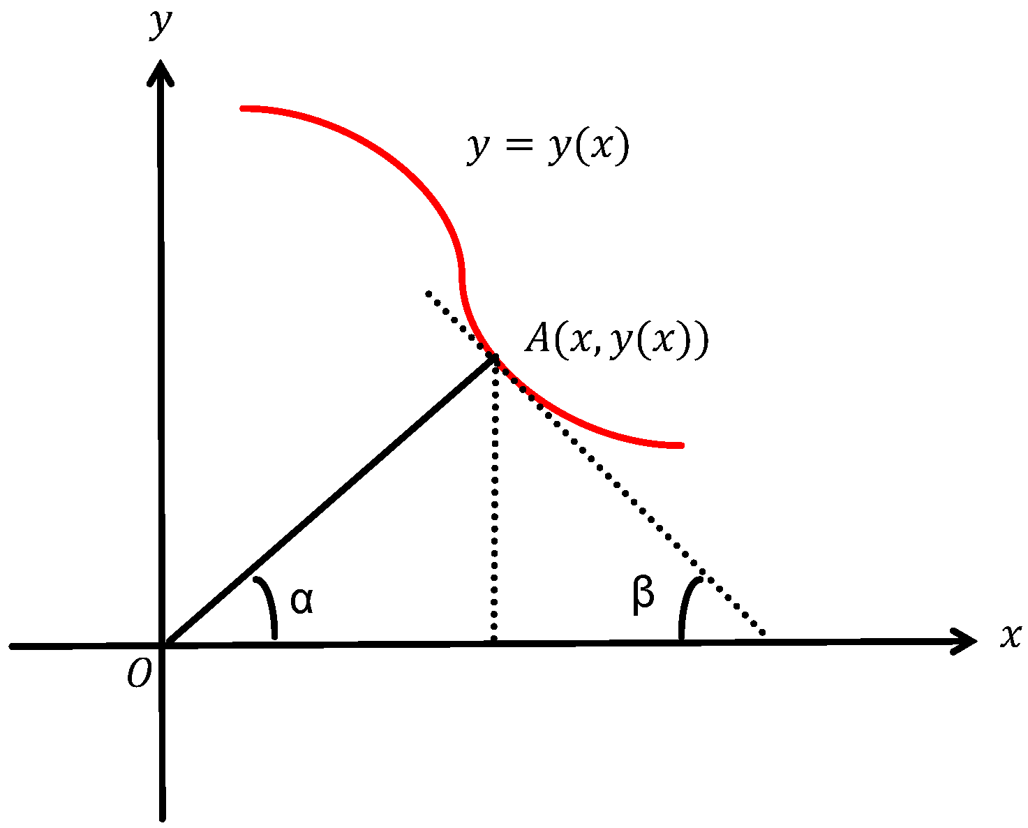
Therefore, the geometric interpretation of the marginal function (derivative function) is the slope of the tangent line at each point on the curve represented by the function . As shown in the Figure 1, take any point on the curve . The tangent to the curve at point forms an angle with the x-axis. , denotes the tangent of the angle that is .

Figure 1.
The geometric meaning of elasticity.
2.2. Elastic Representation of the Derivative and Elastic Inverse Transformation
This section explores the representation of the derivative of elasticity and introduces the elastic inverse transformation method (EITM). They are very useful for solving differential equations.
Lemma 1.
As shown in Section 2.1, it is easy to obtain the following formula:
Lemma 2
(Elastic Inverse Transformation Method). If the elasticity function exists, then the original function
Equation (4) is called an elastic inverse transformation, where .
2.3. General Solution of the Tschebycheff Equation [21]
In the field of ordinary differential equations in mathematics, there is an equation of the following form:
where n is a positive integer, . The generalized solution of this equation is given as
where are arbitrary constant real numbers, is a Tschebycheff polynomial, and is the second Tschebycheff function.
3. Main Theorems and Proofs
This section presents and proves four theorems. Theorem 1 establishes and proves the similar structure of the boundary value problem for the Chebyshev equation, while Theorem 2 conducts a similar analysis for the composite Chebyshev equation boundary value problem. Theorem 3, by combining the elastic transformation method with the conclusion of Theorem 1, solves the similar structure of a class of variable coefficient differential equations; Theorem 4, using the elastic transformation method and the conclusion of Theorem 2, solves the similar structure of a class of variable coefficient differential equation systems.
Theorem 1.
Considering the following boundary problem for the Tschebycheff equation:
where are known real constants, , , and n is a positive integer.
If the above differential equation has a unique solution, the similar construction to this system of equations is expressed as follows:
where are similar kernel functions as follows:
where is called the guiding function for a solution, and it is expressed as follows [25]:
Proof of Theorem 1.
Obviously, the first equation in Equation (8) is a Tschebycheff equation, so the general solution of this equation can be given according to Equation (5) as follows:
This establishes a system of equations in which serve as the undetermined coefficients. Suppose that Equation (8) has a unique solution, the coefficient determinant of this equation, , and
In the above equation, the expression of is determined separately using Equations (11)–(14). Solve the system of equations using Cramer’s rule as follows:
□
Theorem 2.
Consider the following boundary value problem for the composite Tschebycheff equation:
where are known real constants, , , and and are positive integers.
If the above boundary value problem has a unique solution, it can be solved by a similar construction method. The similar construction of its left-region solution can be presented as
A similar construction of its left-region solution can be presented as
where is called the right-region similar kernel function, which is depicted as follows:
where is called the left-region similar kernel function, which is depicted as follows:
where , the guiding function for the solution, can be computed by the following formula [25]:
Proof of Theorem 2.
Clearly, the first two equations in Equation (23) are both Tschebycheff equations. Cccording to Equation (5), the general solution of the two equations can be written as follows:
According to Cramer’s rule, the coefficients , , , and are calculated and simplified as follows:
where
Theorem 3.
Considering the following boundary value problem for a class of differential equations with variable coefficients.
Proof of Theorem 3.
Step 1: Regarding w as the elasticity of a certain non-zero function y to x, from Lemma 1, we have
Step 2: It is apparent that the first differential equation of Equation (46) is a Tschebycheff equation. From Equation (6), the general solution is .
Step 4: By Theorem 1, we can obtain a similar construction to this system of equations is expressed as follows:
where is a similar kernel function, defined as
Step 5: The solution of this equation is found from Lemma 2:
The equation is solved. □
Theorem 4.
The following is a solution of a class of problems reducible to the composite Tschebycheff boundary value problem:
Proof of Theorem 4.
Step 1: Using the elastic down-order transformation of differential equations in boundary problems using Lemma 1, is the elastic function of . Let
where . Bringing Equation (56) into Equation (54) reduces it to the composite Tschebycheff equation boundary value problem. Thus, we can obtain the composite Tschebycheff equation of the following form:
Step 2: Obviously, the first two formulas of Equation (57) are Tschebycheff equations. From Equation (6), the general solutions can be written, respectively, as
Step 3: Constructing the guiding function according to Equations (28)–(31), the guiding functions of the first formula of Equation (57) are constructed as follows:
and the guiding functions of the second formula of Equation (57) are computed as follows:
Step 4: From Theorem 2, a similar structure solution in the region on the left side is calculated as
where is called the left-region similar kernel function, and it is depicted as follows:
The similar structure solution in the region on the right side is derived as
where is called the right-region similar kernel function, and it is depicted as follows:
Step 5: The solution of this equation is found from Lemma 2:
Thus, the equation is solved. □
4. Flowchart
4.1. Flowchart for Solving a Class of Third-Order Nonlinear Variable Coefficient Constant Differential Square Boundary Value Problems Using the Elastic Transformation Method with the Similar Construction Method
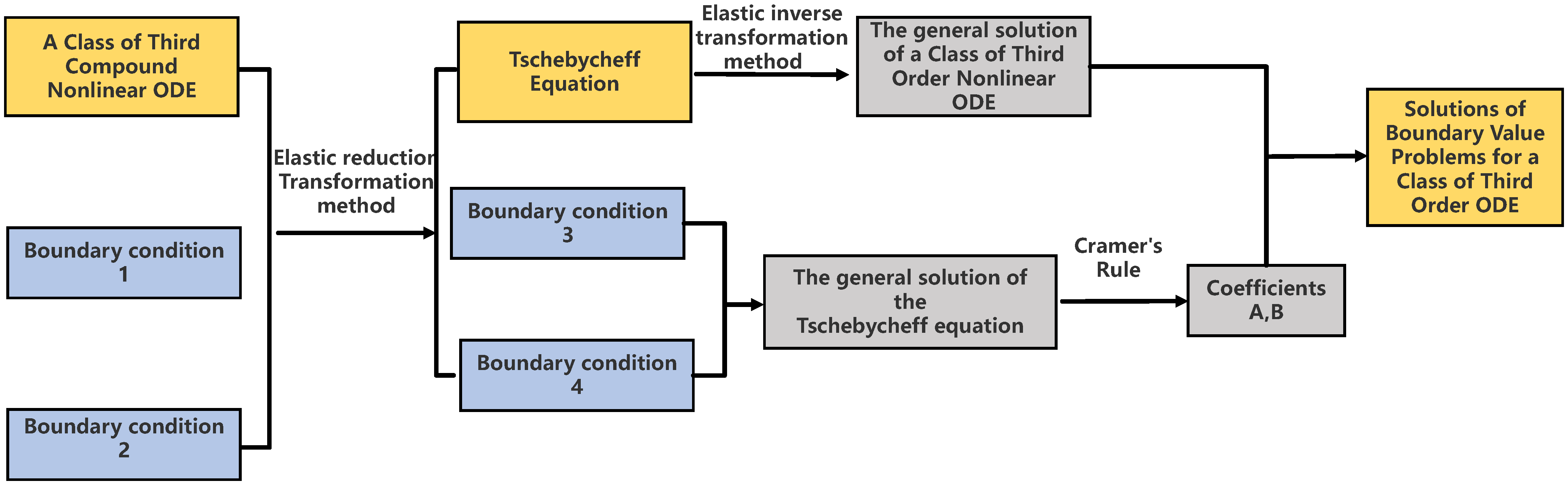
In the Figure 2, it employs the ETM to solve a class of third-order nonlinear ODEs. The key steps are as follows:

Figure 2.
Flowchart for solving a class of third-order differential equations with boundary value problems.
- 1.
- Problem Formulation: Define the original third-order nonlinear ODE along with boundary conditions.
- 2.
- Elastic Transformation: Convert the nonlinear ODE into a Tschebycheff equation using an elastic reduction transformation.
- 3.
- Solve the Tschebycheff Equation: Obtain the general solution under transformed boundary conditions.
- 4.
- Inverse Transformation: Map the solution back to the original nonlinear ODE.
- 5.
- Coefficient Determination: Use Cramer’s law to compute coefficients ensuring boundary condition satisfaction.
- 6.
- Final Solution: Substitute coefficients into the general solution to obtain the final result.
This method streamlines the solution process by transforming a complex nonlinear ODE into a solvable equation and reconstructing its solution efficiently.
4.2. Flowchart for Solving a Class of Third-Order Composite Nonlinear Variable Coefficient Constant Differential Square Boundary Value Problems by the Elastic Transformation Method with the Similar Construction Method
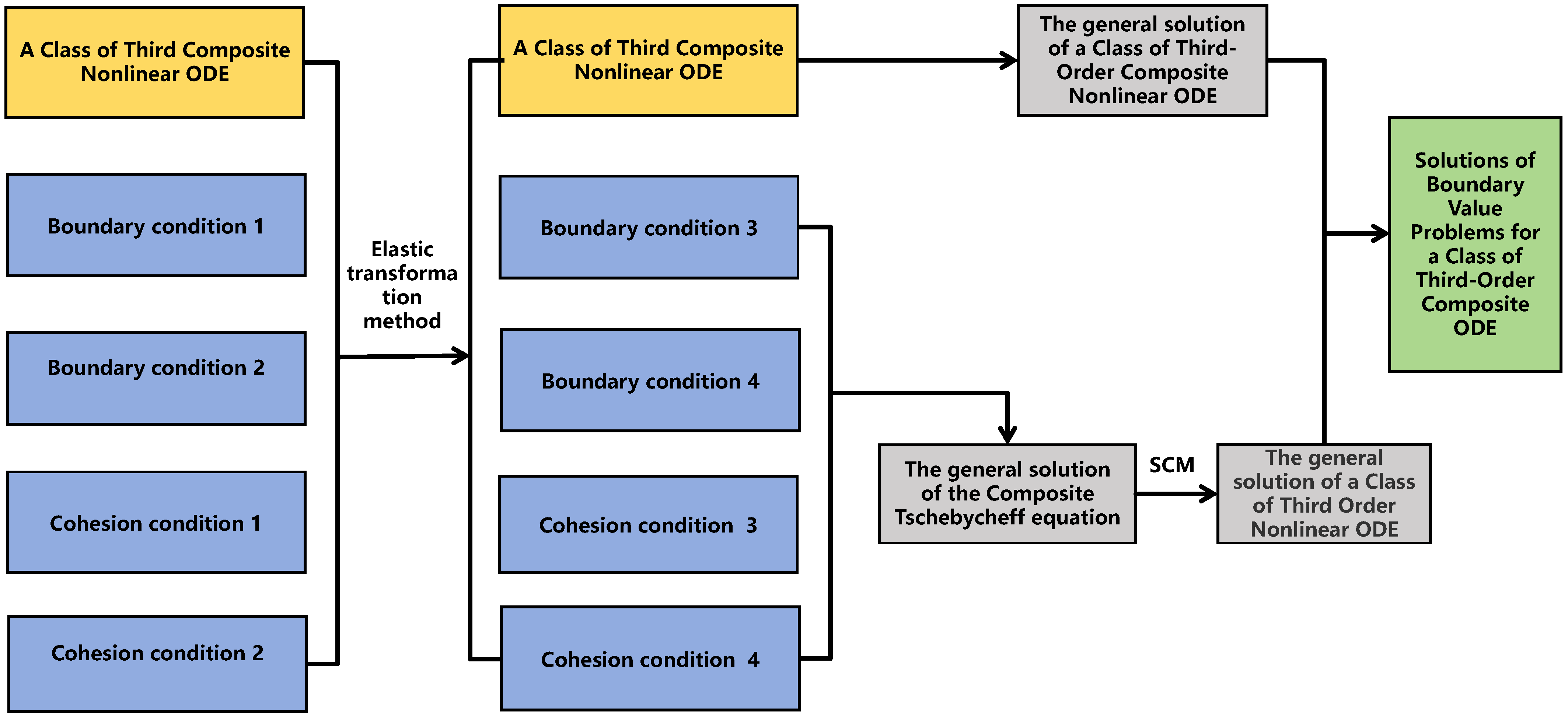
In the Figure 3, it employs the solution process for boundary value problems of third-order composite nonlinear ODEs via the ETM:

Figure 3.
Flowchart for solving a class of third-order composite differential equations with boundary value problems.
- 1.
- Problem Formulation: Set a class of third-order composite nonlinear ODEs as the target, along with two boundary and two cohesion conditions.
- 2.
- Elastic Transformation: Transform the ODEs, obtaining new boundary and cohesion conditions.
- 3.
- Tschebycheff Equation Solution: Solve the composite Tschebycheff equation using the new conditions to obtain its general solution.
- 4.
- Solution Conversion: Employ the SCM method to convert the Tschebycheff equation’s solution to that of the original ODEs.
- 5.
- Final Solution: Derive the boundary value problem solutions based on the converted general solution.
Overall, this approach, considering cohesion conditions and the SCM method, simplifies the solution of complex ODEs through an elastic transformation.
5. Example of Theorem
In this section, we present practical examples to validate the feasibility of the ETM and SCM.
5.1. For a Class of Third-Order Nonlinear Ordinary Differential Equations with Boundary Value Problems
The following equation represents a class of third-order nonlinear ordinary differential equations with boundary value problems:
Step 1: Let . y is the elasticity function of w, which can be calculated according to Theorem 3.
Step 2: Apparently, the first equation of Equation (68) is the Tschebycheff equation of degree . According to Section 2.3, the general solution is .
5.2. For a Class of Third-Order Nonlinear Composite Ordinary Differential Equations with Boundary Value Problems
The following equation represents a class of third-order nonlinear composite ordinary differential equations with boundary value problems:
Step 1: Let . At this point, y is the elasticity function of w, which can be calculated according to Theorem 4.
Step 2: Apparently, the first and second formulas of Equation (78) are Tschebycheff equations of degree . According to Section 2.3, the general solutions of Laguerre equations are, respectively, .
Step 3: Solve the guiding function of the first formula of Equation (78) according to Equation (60):
Solve the guiding function of the second formula of Equation (78) according to Equation (61):
Step 4: Compare Equation (57), i.e., , , , , , , , . From Equation (65) and Equation (63), the right and left similar kernel functions can be obtained.
where is its right-region similar kernel function.
where is its left-region similar kernel function.
According to Equation (62) and Equation (64), the similar structures of the solutions of Equation (78) are computed as
Step 5: From Lemma 2, elastic inverse transformations can be calculated as
6. Curve Analysis
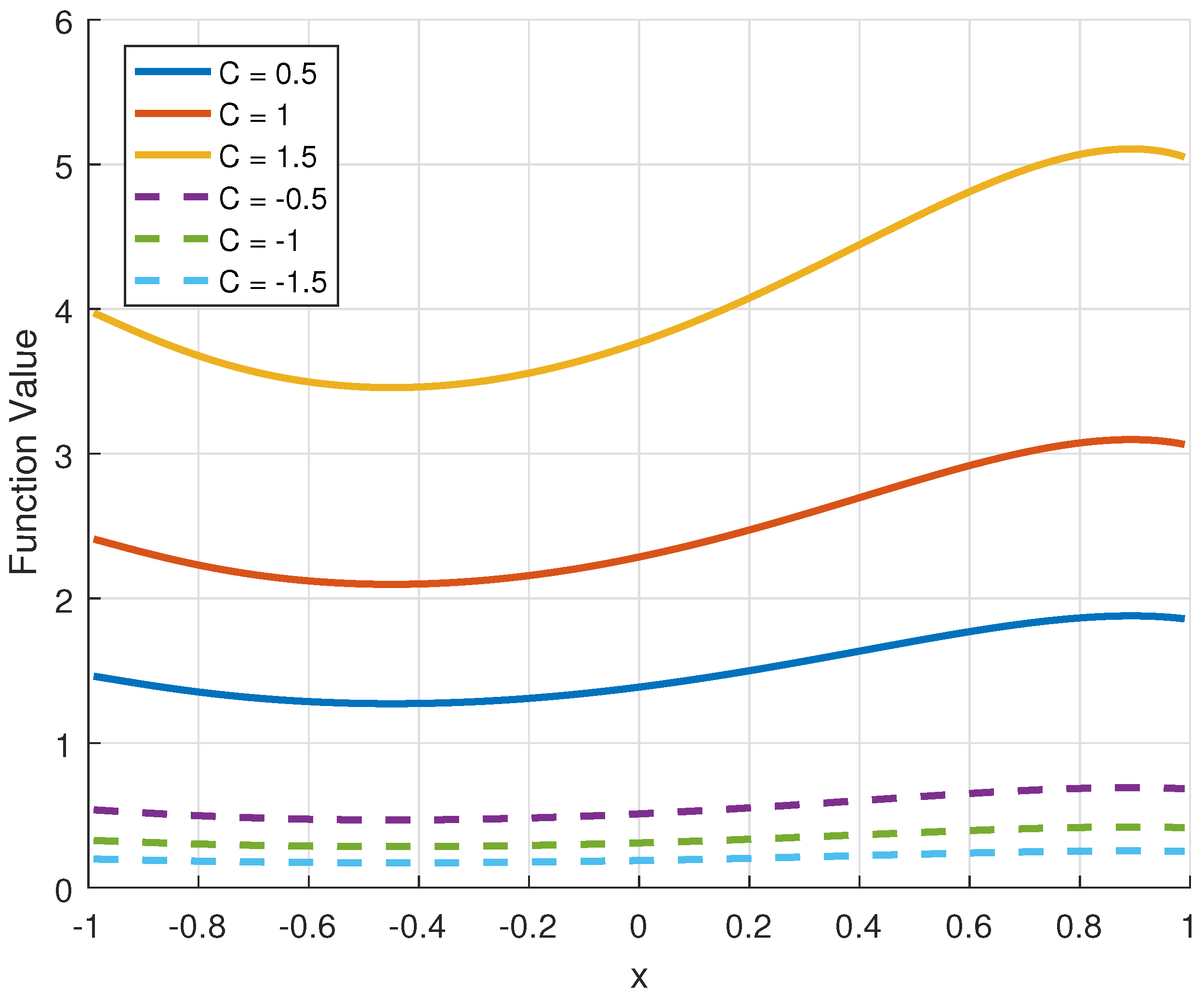
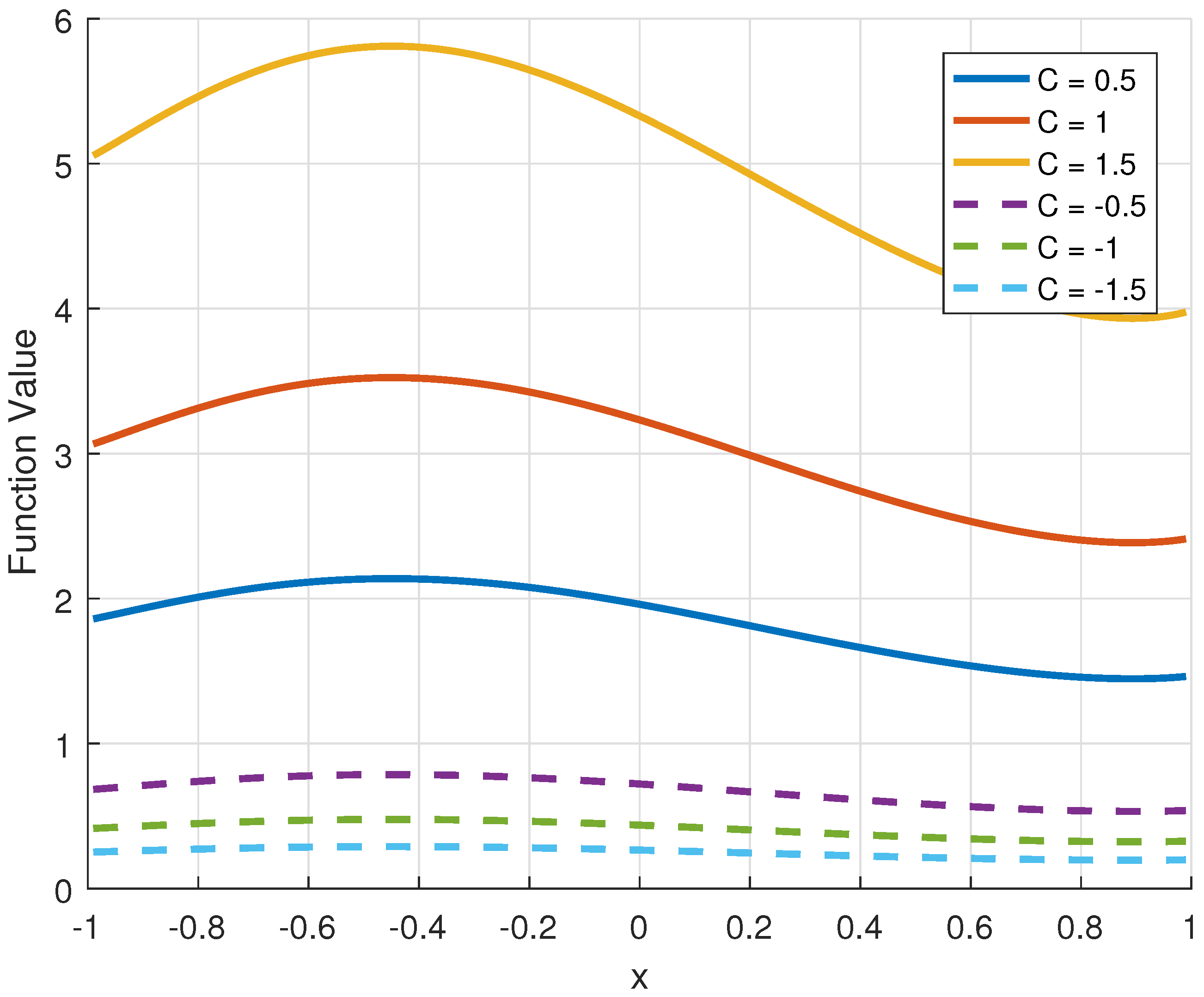
6.1. Considering the Effect of Different C Values on the Curve of the Original Function of a Class of Third-Order Nonlinear Ordinary Differential Equations
In Figure 4, the parameters are . It can be observed that when other parameters are fixed, the parameter C exhibits a consistent influence on the function values . When C is positive, the curves shift upward, and the range of function values increases. Additionally, as C increases, the amplitude of the function’s variation becomes larger, resulting in a steeper overall shape. Conversely, when C is negative, the curves shift downward, and the function values remain relatively small. As C decreases further, the variation in the function diminishes, leading to a smoother overall trend. This indicates that positive values of C have a more pronounced effect on the function, whereas changes in negative values of C have a relatively smaller impact on the function’s shape.
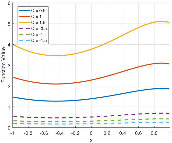
Figure 4.
The effect of different C values on the curve of the original function.
For all C values, the function exhibits non-monotonic behavior within the interval . It reaches relatively high values near , flattens around , and rises again near . These variations reflect the significant role of the C parameter in modulating the nonlinear shape of the function.
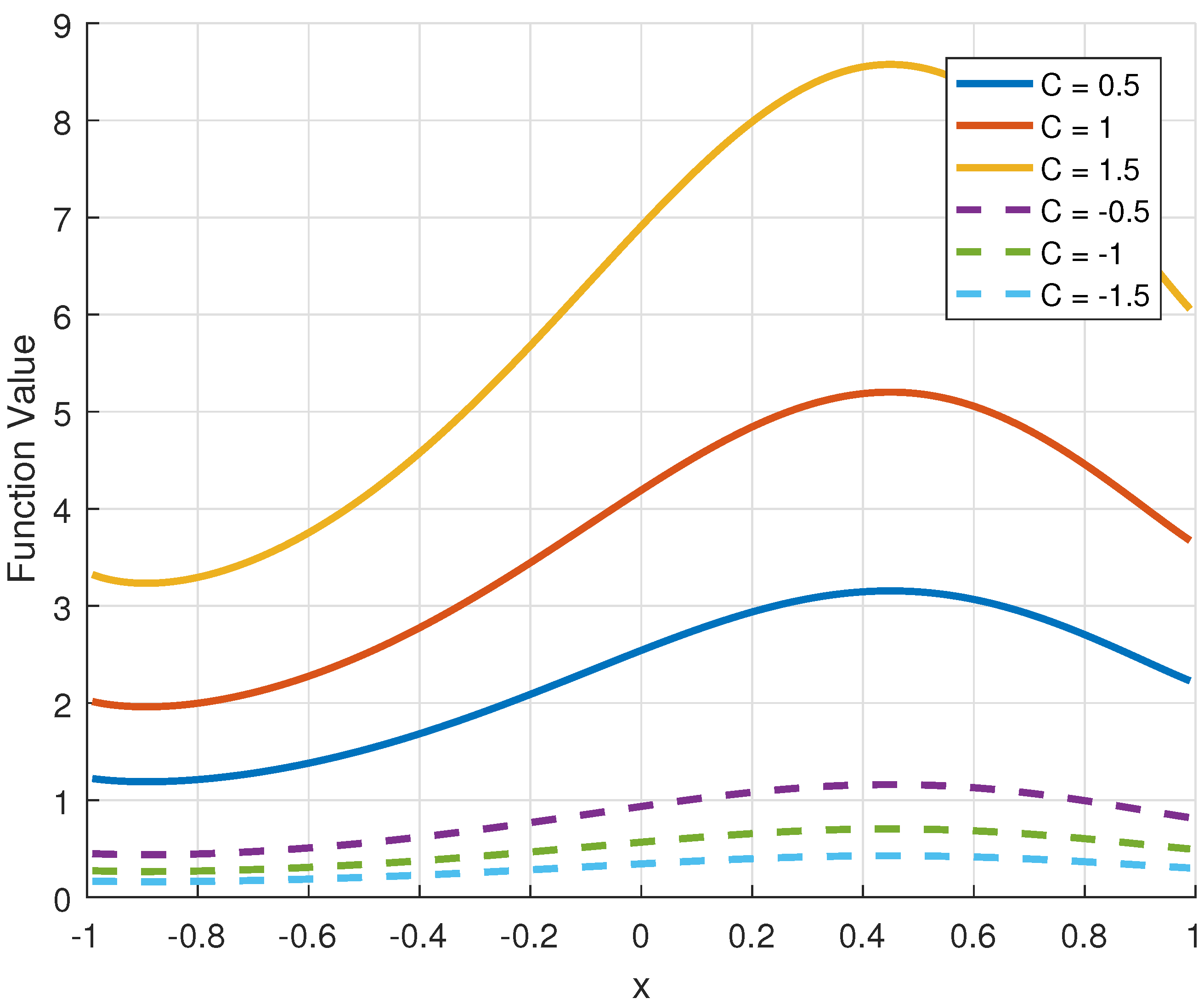
6.2. Considering the Effect of Different Initial C Values in the Region on the Left Side on the Curve of the Original Function of a Class of Third-Order Composite Nonlinear Ordinary Differential Equations
In Figure 5, the parameters are . It can be clearly seen that when other parameters are fixed, the six curves have the same trend. When C assumes positive values, it induces an upward shift in the curve. Concurrently, as the magnitude of C increases, there is an expansion in the range of function values. The curves exhibit pronounced non-monotonic behavior, reaching a peak around before slightly decreasing. Conversely, negative C values shift the curve downward, and as C decreases, the range of function values contracts, resulting in a more subdued and smoother shape. The non-monotonic behavior is less prominent for negative C. Overall, enhances the curve’s nonlinearity and amplitude, while results in flatter and lower curves.
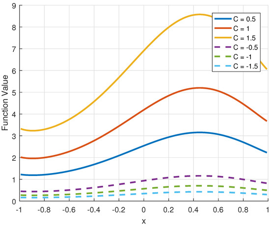
Figure 5.
The effect of different C values on the curve of the solution on the region on the left side of the original function.
6.3. Considering the Effect of Different C Values in the Region on the Right Side on the Curve of the Original Function of a Class of Third-Order Composite Nonlinear Ordinary Differential Equations
In Figure 6, the parameters are . It is noticeable that with other parameters held constant, the C parameter has a uniform impact on the function values . When , the curve shifts upward, and as C increases, the range of function values expands, with the curve exhibiting pronounced non-monotonic behavior, peaking around and then gradually decreasing. Conversely, when , the curve shifts downward, and as C decreases, the range of function values contracts, resulting in flatter and smoother curves with less pronounced non-monotonicity. Generally speaking, positive C values contribute to an increase in the curve’s fluctuation range and an enhancement of its nonlinear traits. In contrast, negative C values have the effect of restraining these traits, causing the curve to take on a more symmetric and smoother appearance.
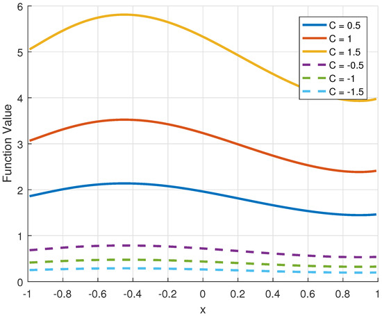
Figure 6.
The effect of different C values on the curve of the solution in the region on the right side of the original function.
7. Conclusions
- 1.
- This study employs the elastic transformation method (ETM) to transform the third-order boundary value problem and composite third-order nonlinear ordinary differential equations into second-order Tschebycheff equations. The boundary value problem of the Tschebycheff equation is then solved using the similar construction method (SCM). Finally, by applying the inverse elastic transformation method (EITM), the solution to the original third-order nonlinear ordinary differential equation is obtained.
- 2.
- The ETM effectively reduces the order of higher-order differential equations, simplifying their solution process. In contrast, the EITM elevates a lower-order equation to a higher order, transforming it into a solvable form. Moreover, the SCM ensures a systematic approach, eliminating the need for cumbersome computational procedures. The integration of these methods provides a novel strategy for solving nonlinear differential equations with variable coefficients.
8. Discussion
Although the ETM has many advantages, it is mainly designed for differential equations with specific types of variable coefficients. For example, if the variable coefficients in a differential equation do not follow a regular pattern or exhibit highly irregular behavior, these methods may not be applicable. However, both the ETM and the SCM can significantly simplify the solution process of higher-order differential equations and provide a new approach for solving nonlinear differential equations. These methods expand the solvable class of ordinary differential equations and offer convenience to scholars who will study differential equations in the future. In addition, in the teaching of the ordinary differential equations’ course, we applied this method to the solution of ordinary differential equations with variable coefficients, thus expanding the course content.
Author Contributions
Conceptualization, P.Z. and J.L.; methodology, P.Z.; software, P.Z.; validation, P.Z., J.L. and J.X.; formal analysis, P.Z.; investigation, J.L.; resources, J.L.; data management, J.L.; writing—original draft preparation, P.Z.; writing—review and editing, P.Z., J.L. and J.X.; visualization, P.Z.; supervision, P.Z.; project administration, P.Z. All authors have read and agreed to the published version of the manuscript.
Funding
This research was funded by the Data Analysis Technology Consulting project (No. ZH20250070) and funded by Sichuan Qianchengxin Technology Co., Ltd., the Quality Project of Graduate Education Xihua University (No. YJSKC202204), and the Scientific Research Fund of the Sichuan Provincial Science and Technology Department, China (Grant No. 2015JY0245).
Data Availability Statement
The datasets generated and analyzed during the current study are available from the corresponding author upon reasonable request.
Acknowledgments
We thank the referees for pointing out some misprints and for their helpful suggestions.
Conflicts of Interest
The authors declare no conflicts of interest.
References
- Wang, F.F.; Jiang, Z.S. Explicit Solutions of Some Nonlinear Evolution Equations through Separation of Variables. Sch. Math. 2024, 40, 58–62. [Google Scholar]
- Zhao, L.L. Integral Factors and Integral Factor Method. Sch. Math. Stat. 2023, 26, 19–22+25. [Google Scholar]
- Öziş, T.; Ağırseven, D. He’s homotopy perturbation method for solving heat-like and wave-like equations with variable coefficients. Phys. Lett. A 2008, 372, 5944–5950. [Google Scholar]
- Verma, A.K.; Kumar, N. A note on variation iteration method with an application on Lane–Emden equations. Eng. Comput. 2021, 38, 3932–3943. [Google Scholar]
- Jaiswal, J.P. Some Class of Third-and Fourth-Order Iterative Methods for Solving Nonlinear Equations. J. Appl. Math. 2014, 2014, 817656. [Google Scholar]
- Li, J.X.; Li, L. The Application of Variable Substitution in Ordinary Differential Equations. Sch. Math. Baoshan Univ. 2016, 35, 51–54. [Google Scholar]
- Liu, Q. Solutions and Integrability Analysis of Two Classes of Nonlinear Differential Equations. Master’s Thesis, North China Electric Power University, Beijing, China, 2021. [Google Scholar]
- Ouyang, T. Application of Three Methods in Solving Nonlinear Partial Differential Equations. Master’s Thesis, Xinjiang Normal University, Ürümqi, China, 2022. [Google Scholar]
- Li, S.C.; Yi, L.Z.; Zheng, P.S. The Similar Structure of Differential Equation on Fixed Solution Problem. J. Sichuan Univ. (Nat. Sci. Ed.) 2006, 43, 933–934. [Google Scholar]
- Li, S.C. The Similarity Structuring Method of Boundary Value Problems for Composite Differential Equations. J. Xihua Univ. Nat. Sci. 2013, 32, 27–31. [Google Scholar]
- Li, H.E.; Dong, X.X.; Li, S.C.; Fan, C.Y. A New Method and Applications of the Boundary Value Problem of Differential Equation. Adv. Mater. Res. 2014, 937, 695–699. [Google Scholar] [CrossRef]
- Shi, J. The Constructive Method and Its Applications of Solutions for the Boundary Value Problem of Composite Second-Order Differential Equation. Master’s Thesis, Xihua University, Chengdu, China, 2014. (In Chinese). [Google Scholar]
- Zheng, P.; Li, S.; Leng, L.; Gui, D. Similar Construction Method of Boundary Value Problems of a Nonlinear Composite Modified Bessel Equations. J. Xinyang Norm. Univ. (Nat. Sci. Ed.) 2014, 27, 490–492+504. [Google Scholar]
- Dong, X.X.; Liu, Z.B.; Li, S.C. Similar Constructing Method for Solving Nonlinear Spherical Seepage Model with Quadratic Pressure Gradient of Three-region Composite Fractal Reservoir. Comput. Appl. Math. 2019, 38, 83. [Google Scholar]
- Sheng, C.C.; Zhao, J.Z.; Li, Y.M.; Li, S.C.; Jia, H. Similar Construction Method of Solution for Solving the Mathematical Model of Fractal Reservoir with Spherical Flow. J. Appl. Math. 2013, 2013, 219218. [Google Scholar]
- Xu, L.; Liu, X.; Liang, L.; Li, S.; Zhou, L. The Similar Structure Method for Solving the Model of Fractal Dual-Porosity Reservoir. Math. Prob. Eng. 2013, 2013, 954106. [Google Scholar]
- Rosa, A.J.; Horne, R.H.N. Automated Type-Curve Matching in Well Test Analysis Using Laplace Space Determination of Parameter Gradients. In Proceedings of the SPE Annual Technical Conference and Exhibition, San Francisco, CA, USA, 5–8 October 1983. [Google Scholar]
- Roumboutsos, A.; Stewart, G. A Direct Deconvolution or Convolution Algorithm for Well Test Analysis. In Proceedings of the SPE Annual Technical Conference and Exhibition, Houston, TX, USA, 2–5 October 1988. [Google Scholar]
- Sahimi, M.; Yortsos, Y.C. Applications of Fractal Geometry to Porous Media: A Review. In Proceedings of the Annual Fall Meeting of the Society of Petroleum Engineers, New Orleans, LA, USA, 3–6 October 1990. [Google Scholar]
- Li, S.C.; He, Q.; Dong, X.X. The Elasticity of the Outer Boundary and the Solution of Two-Region Composite Reservoir Seepage Model. Pet. Sci. Technol. 2022, 40, 2773–2791. [Google Scholar] [CrossRef]
- Zheng, P.; Luo, J.; Li, S.; Dong, X. Elastic Transformation Method for Solving Ordinary Differential Equations with Variable Coefficients. AIMS Math. 2022, 7, 1307–1320. [Google Scholar] [CrossRef]
- Lin, F.; Li, S.; Shao, D.; Fu, X.; Liu, P.; Gui, Q. Elastic Transformation Method for Solving the Initial Value Problem of Variable Coefficient Nonlinear Ordinary Differential Equations. AIMS Math. 2022, 7, 11972–11991. [Google Scholar]
- Fan, L. Research on Solvable Classes of Riccati Equation Based on Elastic Transformation. Ph.D. Thesis, Xihua University, Chengdu, China, 2023. [Google Scholar]
- Jiang, T.; Zheng, P.; Xu, L.; Leng, L. Application of Elastic Transformation Method and Similarity Construction Method in Solving Ordinary Differential Equations. J. Appl. Math. Comput. 2023, 70, 175–195. [Google Scholar] [CrossRef]
- Xia, W.; Li, S.; Gui, D. Similar Structured Method of Solution to Boundary Value Problems of the Composite Tschebyscheff System. J. Shaanxi Univ. Technol. (Nat. Sci. Ed.) 2015, 31, 69–74. [Google Scholar]
Disclaimer/Publisher’s Note: The statements, opinions and data contained in all publications are solely those of the individual author(s) and contributor(s) and not of MDPI and/or the editor(s). MDPI and/or the editor(s) disclaim responsibility for any injury to people or property resulting from any ideas, methods, instructions or products referred to in the content. |
© 2025 by the authors. Licensee MDPI, Basel, Switzerland. This article is an open access article distributed under the terms and conditions of the Creative Commons Attribution (CC BY) license (https://creativecommons.org/licenses/by/4.0/).