Article

Convergence Analysis of Jarratt-like Methods for Solving Nonlinear Equations for Thrice-Differentiable Operators

1
Department of Mathematical and Computational Sciences, National Institute of Technology Karnataka, Surathkal, Mangalore 575025, India
2
Department of Mathematical Sciences, Cameron University, Lawton, OK 73505, USA
3
College of Computing and Engineering, Nova Southeastern University, Fort Lauderdale, FL 33328, USA
*
Authors to whom correspondence should be addressed.
AppliedMath 2025, 5(2), 38; https://doi.org/10.3390/appliedmath5020038
Submission received: 17 January 2025 / Revised: 25 February 2025 / Accepted: 24 March 2025 / Published: 3 April 2025

Abstract

:
The main goal of this paper is to study Jarratt-like iterative methods to obtain their order of convergence under weaker conditions. Generally, obtaining the p t h -order convergence using the Taylor series expansion technique needed at least p + 1 times differentiability of the involved operator. However, we obtain the fourth- and sixth-order for Jarratt-like methods using up to the third-order derivatives only. An upper bound for the asymptotic error constant (AEC) and a convergence ball are provided. The convergence analysis is developed in the more general setting of Banach spaces and relies on Lipschitz-type conditions, which are required to control the derivative. The results obtained are examined using numerical examples, and some dynamical system concepts are discussed for a better understanding of convergence ideas.

1. Introduction

In general, finding an analytical (or closed-form) solution to the equation
Ψ ( x ) = 0
is not achievable, where Ψ : Ω X Y is a nonlinear operator defined on Banach spaces X and Y, and Ω is an open convex subset of X. However, one can obtain an approximate solution using iterative methods. In 1685, Newton introduced a basic idea for solving polynomial equations, and later in 1690, Raphson gave a proper shape to the method, which is known as the Newton–Raphson method [1,2,3,4,5,6,7] given by
x 0 X , x k + 1 = x k Ψ ( x k ) 1 Ψ ( x k ) , k = 0 , 1 , 2 , .
The Newton method (2) was extended to Banach spaces by Kantorovich [2]. Many altered versions of (2) were given by several authors [1,8,9,10,11,12] to improve the order of convergence. The Jarratt method [9] is one of them, which is best-known among the fourth-order methods, defined by
y k = x k 2 3 Ψ ( x k ) 1 Ψ ( x k ) , A k = 3 Ψ ( y k ) Ψ ( x k ) , x 0 X x k + 1 = x k 1 2 A k 1 3 Ψ ( y k ) + Ψ ( x k ) Ψ ( x k ) 1 Ψ ( x k ) , k = 0 , 1 , 2 , .
Sharma and Arora [13] studied the convergence analysis of the Jarratt-like method given by
y k = x k 2 3 Ψ ( x k ) 1 Ψ ( x k ) x k + 1 = x k 23 8 I + Ψ ( x k ) 1 Ψ ( y k ) 3 I + 9 8 Ψ ( x k ) 1 Ψ ( y k ) Ψ ( x k ) 1 Ψ ( x k ) .

1.1. Motivation

  • Proving the order of convergence of an iterative method is not a straightforward task. In [13], the authors proved that method (4) has an order of convergence of four by using the Taylor series expansion for the operators, which are at least five times differentiable. Even though higher-order derivatives of the involved operators are not present in the structure of the iterative methods, one needs the existence of higher-order derivatives to obtain the convergence order, which limits their applicability. For example, consider the equation λ ( s ) = 0 , s [ 0.5 , 0.5 ] , where λ ( s ) = s 6 cos ( 1 / s ) , s 0 and 0 otherwise. It is observed that λ ( 4 ) ( s ) = 360 s 2 cos 1 / s + 240 s sin ( 1 / s ) 72 cos 1 / s 12 / s sin 1 / s , s 0 is unbounded at s = 0 [ 0.5 , 0.5 ] and λ ( 0 ) = 0 . Therefore, method (4) cannot guarantee the convergence if one uses the analysis in [13].
  • Some more weaknesses in [13] can be improved. For example, the results related to method (4) are given for Euclidean spaces, and no information is provided about the asymptotic error constant.
  • The most important semi-local convergence analysis has not been given.
  • A set that contains all suitable initial points for convergence of the process is not provided in earlier studies.
All the above-discussed issues are addressed by our techniques in this work.

1.2. Originality

The highlights and novelty of our work are as follows:
(I)
We prove that method (4) has an order of convergence of at least four without using the Taylor series expansion, only considering the existence of the third-order differentiability of the involved operator.
(II)
We present a ball of convergence and address the uniqueness of the solution, which is not provided in earlier works.
(III)
We extend method (4) to a sixth-order method given by
y k = x k 2 3 Ψ ( x k ) 1 Ψ ( x k ) z k = x k 23 8 I + Ψ ( x k ) 1 Ψ ( y k ) 3 I + 9 8 Ψ ( x k ) 1 Ψ ( y k ) Ψ ( x k ) 1 Ψ ( x k ) x k + 1 = z k 2 I Ψ ( x k ) 1 Ψ ( z k ) Ψ ( x k ) 1 Ψ ( z k ) .
(IV)
Semi-local convergence analysis is given for methods (4) and (5), which is not included in earlier studies.
(V)
An upper bound for the asymptotic error constant is provided.
(VI)
The selection of initial points not previously available is now known.
(VII)
The analysis is conducted in Banach spaces.
Consequently, there is advanced knowledge of the number of iterations to be calculated for a certain error tolerance. This information is not available in previous works. Notice that although our technique with Taylor series is demonstrated using (4) or (5) due to its generality, it can be applied to extend the applicability of other methods analogously. The limitations of the present approach are as follows:
(a)
The convergence conditions are sufficient but not necessary. It will be interesting to also find necessary conditions. This will be the direction of future research, even if we will have to impose additional conditions.
(b)
We can see if the second Lipschitz-type condition ( A 2 ) for the semi-local case or the Lipschitz-type conditions on second and third derivative (see ( A 4 ), ( A 5 ), respectively) for the local convergence case can be weakened.
The rest of the paper is organized as follows: Section 2 contains some related basic concepts. We discuss the semi-local convergence analysis in Section 3, and in Section 4, we discuss the local convergence analysis for methods (4) and (5). We include some examples for validating our results in Section 5, and the dynamical concepts are discussed in (6). Finally, concluding remarks are given in Section 7.

2. Basic Concepts

We use the following notations, B ( X , Y ) = { F : X Y | F is a bounded linear operator}, B ( x , λ ) = { y X :   y x   < λ } , and B [ x , λ ] = { y X :   y x   λ } , where x X and λ > 0 .
Definition 1
(Majorizing Sequence [14]). Let { α k } k N be a sequence in a Banach space X and { γ k } k N be a real sequence. We say { γ k } k N is a majorizing sequence of { α k } k N if α k + 1 α k   γ k + 1 γ k , k 0 .
Theorem 1
(Intermediate Value Theorem [3]). Let h be a real-valued continuous function on a closed and bounded interval I in R . If a , b I , a < b and 0 h ( a ) , h ( b ) or h ( b ) , h ( a ) , then there exists at least one c ( a , b ) such that h ( c ) = 0 .
Note that if a given function h is non-decreasing with h ( a ) < 0 and lim s b h ( s ) = + , then there exists a point s 0 in a left neighborhood of b such that h ( s 0 ) > 0 . So, by Theorem 1, there exists at least one point c 0 ( a , s 0 ) ( a , b ) such that h ( c 0 ) = 0 .
Definition 2
(Fréchet Derivative [4]). Let X and Y be Banach spaces and O X be an open set. A map Δ : O Y is said to be Fréchet differentiable at t 0 O if there exists a bounded linear operator Δ ( t 0 ) : X Y , i.e., Δ ( t 0 ) B ( X , Y ) such that
lim h X , h 0 Δ ( t 0 + h ) Δ ( t 0 ) Δ ( t 0 ) ( h ) h = 0 .
Theorem 2
(Integral Form of Mean Value Theorem [4,5]). Let Δ : Ω X Y be a Fréchet differentiable operator on Ω and Δ be Riemann integrable on the line segment { x + θ ( y x ) : 0 θ 1 } , x , y Ω ; then,
Δ ( y ) Δ ( x ) = 0 1 Δ x + θ ( y x ) d θ ( y x ) .
Lemma 1
(Banach Lemma for Invertible operator [6]). Let Δ B ( X , X ) with Δ   ϱ < 1 . Then, the inverse operator of I Δ exists and ( I Δ ) 1   1 1 ϱ , where I is an identity operator.
Definition 3
(Order of Convergence [15]). Let ξ , x k X , for k = 0 , 1 , 2 , 3 , satisfying the following conditions:
(i) 
lim k x k ξ = 0 ,
(ii) 
There exists τ > 0 , n 0 N , and p [ 1 , ) such that x k + 1 ξ   τ x k ξ p , k n 0 ;
then, we say the sequence { x k } k N is convergent to ξ with an order of at least p. The asymptotic error constant (AEC) is defined as C p : = lim k x k + 1 ξ x k ξ p .

3. Semi-Local Convergence Analysis of (4) and (5)

In this section, we analyze the semi-local convergence of methods (4) and (5) under the following conditions:
( A 1 )
There exists x 0 Ω and ϖ > 0 such that Ψ ( x 0 ) 1 B ( Y , X ) with 2 3 Ψ ( x 0 ) 1 Ψ ( x 0 ) ϖ .
( A 2 )
There exists L 0 > 0 and an invertible operator T B ( X , Y ) such that
T 1 Ψ ( x ) T L 0 x x 0 , x Ω .
and the Lipschitz-like condition
T 1 Ψ ( x ) Ψ ( y ) L 0 x y , x , y Ω * = B ( x 0 , λ * ) Ω ,
where λ * is given in Lemma 2.
( A 3 )
L 0 λ * < 1 2 and B ( x 0 , λ * ) Ω .
Observation 1.
(i) 
The operator T can be considered I (the identity operator) or Ψ ( x 0 ) . Other choices are possible if conditions ( A 1 ) and ( A 2 ) are satisfied.
(ii) 
By condition ( A 2 ), we have
T 1 Ψ ( x )   1 + L 0 x x 0 , x Ω .
(iii) 
From conditions ( A 2 ) and ( A 3 ), we obtain
T 1 Ψ ( x ) T L 0 x x 0 < 1 , x B [ x 0 , λ * ] .
By using Lemma 1, the operator T 1 Ψ ( x ) is invertible and
Ψ ( x ) 1 T 1 1 L 0 x x 0 , x B [ x 0 , λ * ] .
(iv) 
Using (ii) and (iii), we obtain
Ψ ( x ) 1 Ψ ( y ) Ψ ( x ) 1 T T 1 Ψ ( y ) 1 + L 0 y x 0 1 L 0 x x 0 , x , y B [ x 0 , λ * ] .
  • Let us define two scalar sequences { a k } k N and { b k } k N by
    a 0 = 0 , b 0 = ϖ , b k = a k + 1 3 ( 1 L 0 a k ) L 0 ( a k a k 1 ) 2 + ( 1 + L 0 a k 1 ) 3 ( a k b k 1 ) + a k a k 1 , a k + 1 = b k + 3 2 53 24 + 1 + L 0 b k 1 L 0 a k 3 + 9 ( 1 + L 0 b k ) 8 ( 1 L 0 a k ) ( b k a k ) .
Lemma 2.
If L 0 a k < 1 , k N , then, both the sequences { a k } and { b k } are convergent to a unique λ * 0 , 1 L 0 .
Proof. 
Suppose that L 0 a k < 1 , k N ; then { a k } k N is bounded above by 1 L 0 . Since a k and b k are non-negative, satisfying a k b k a k + 1 , k N the sequence { a k } k N is monotonically increasing and { b k } k N is squeezed by { a k } k N . So, by Theorem 3.3.2 ([3], p. 71), { a k } k N converges to some λ * and by the Squeeze Theorem, 3.2.7 ([3], p. 66), we obtain lim k a k = lim k b k = λ * . □
Theorem 3.
If the conditions ( A 1 ) ( A 3 ) are satisfied, then the sequence { x k } k N generated by the method (4) with the initial vector x 0 Ω is well defined, i.e., x k B [ x 0 , λ * ] , k N , and converges to α * B [ x 0 , λ * ] with Ψ ( α * ) = 0 . Furthermore, α * x k   λ * a k , k N .
Proof. 
In order to complete the proof, we prove the following inequalities:
y k x k b k a k
x k + 1 y k a k + 1 b k , k N .
This can be achieved by the method of induction. Condition ( A 1 ), a 0 = 0 and b 0 = ϖ , gives us
y 0 x 0   = 2 3 Ψ ( x 0 ) 1 Ψ ( x 0 ) ϖ = b 0 a 0 λ * .
This implies that y 0 B [ x 0 , λ * ] . From method (4) and Equation (9), we have
x 1 y 0 53 24 + Ψ ( x 0 ) 1 Ψ ( y 0 ) 3 + 9 8 Ψ ( x 0 ) 1 Ψ ( y 0 ) Ψ ( x 0 ) 1 Ψ ( x 0 ) 3 2 53 24 + ( 1 + L 0 y 0 x 0 ) 3 + 9 8 ( 1 + L 0 y 0 x 0 ) y 0 x 0 3 2 53 24 + ( 1 + L 0 ( b 0 a 0 ) 3 + 9 8 1 + L 0 ( b 0 a 0 ) ( b 0 a 0 ) .
From the definition of a 1 , we have x 1 y 0   a 1 b 0 , and then since a 0 = 0 and a 1 λ * , we have
x 1 x 0     x 1 y 0 + y 0 x 0   a 1 a 0 λ * .
So, x 1 B [ x 0 , λ * ] . Now, assume that Equations (10) and (11) hold for k = 0 , 1 , 2 , , m 1 and x k , y k 1 B [ x 0 , λ * ] , for k = 1 , 2 , , m . Then, x m x m 1   a m a m 1 . By using Theorem 2 and the relation Ψ ( x m 1 ) = 3 2 Ψ ( x m 1 ) ( y m 1 x m 1 ) , we obtain
Ψ ( x m ) = Ψ ( x m ) Ψ ( x m 1 ) Ψ ( x m 1 ) ( x m x m 1 ) + Ψ ( x m 1 ) ( x m x m 1 ) + Ψ ( x m 1 ) = 0 1 Ψ x m 1 + θ ( x m x m 1 ) Ψ ( x m 1 ) d θ ( x m x m 1 ) + Ψ ( x m 1 ) ( x m x m 1 ) 3 2 Ψ ( x m 1 ) ( y m 1 x m 1 ) = 0 1 Ψ x m 1 + θ ( x m x m 1 ) Ψ ( x m 1 ) d θ ( x m x m 1 ) + 3 2 Ψ ( x m 1 ) ( x m y m 1 ) 1 2 Ψ ( x m 1 ) ( x m x m 1 ) .
Condition ( A 2 ) and Equation (7) give us
T 1 Ψ ( x m ) 0 1 T 1 Ψ x m 1 + θ ( x m x m 1 ) Ψ ( x m 1 ) d θ x m x m 1 + 3 2 T 1 Ψ ( x m 1 ) x m y m 1 + 1 2 T 1 Ψ ( x m 1 ) x m x m 1 L 0 0 1 θ d θ x m x m 1 2 + 3 2 ( 1 + L 0 x m 1 x 0 ) x m y m 1 + 1 2 ( 1 + L 0 x m 1 x 0 ) x m x m 1 1 2 L 0 ( a m a m 1 ) 2 + 1 2 ( 1 + L 0 a m 1 ) 3 ( a m b m 1 ) + a m a m 1 .
Then, using Equation (8) and the relation between a m and b m , we obtain
y m x m 2 3 Ψ ( x m ) 1 Ψ ( x m ) 2 3 Ψ ( x m ) 1 T T 1 Ψ ( x m ) 2 3 1 1 L 0 x m x 0 T 1 Ψ ( x m ) 1 3 ( 1 L 0 a m ) [ L 0 ( a m a m 1 ) 2 + ( 1 + L 0 a m 1 ) ( 3 ( a m b m 1 ) + a m a m 1 ) ] = b m a m .
Here, we have x m x 0   j = 1 m x j x j 1 j = 1 m ( a j a j 1 ) = a m a 0 . Then, since a 0 = 0 and λ * is a least upper bound for { b k } k N , y m x 0     y m x m + x m x 0   b m a m + a m a 0 = b m λ * . This implies that y m B [ x 0 , λ * ] . From Equation (9), we have
Ψ ( x m ) 1 Ψ ( y m ) 1 + L 0 y m x 0 1 L 0 x m x 0 1 + L 0 b m 1 L 0 a m .
By using Equations (4) and (12), we have
x m + 1 y m 53 24 + Ψ ( x m ) 1 Ψ ( y m ) 3 + 9 8 Ψ ( x m ) 1 Ψ ( y m ) × Ψ ( x m ) 1 Ψ ( x m ) 3 2 53 24 + 1 + L 0 b m 1 L 0 a m 3 + 9 ( 1 + L 0 b m ) 8 ( 1 L 0 a m ) ( b m a m ) = a m + 1 b m .
Then, we obtain x m + 1 x 0     x m + 1 y m + y m x 0   a m + 1 b m + b m a 0 = a m + 1 λ * and, hence, x m + 1 B [ x 0 , λ * ] . So, by the method of induction, we prove x k , y k 1 B [ x 0 , λ * ] and Equations (10) and (11) for all k N . From this, we obtain
x k + 1 x k x k + 1 y k + y k x k a k + 1 b k + b k a k = a k + 1 a k , k N { 0 } .
By Definition 1, the scalar sequence { a k } k N is a majorizing sequence for { x k } k N , and then Theorem 1.20 ([14], p. 17) implies that the sequence { x k } k N converges to some α * B [ x 0 , λ ] . Note that the sequence { Ψ ( x k ) } k N is bounded and lim k y k x k = 0 . The relation Ψ ( x k ) = 3 2 Ψ ( x k ) ( y k x k ) and the continuity of Ψ imply that Ψ ( α * ) = 0 . Finally, from Equation (13), we obtain α * x k   λ * a k , k N . □
Next, we discuss the semi-local convergence analysis of (5). Let us define scalar sequences { a k } k N , { b k } k N , and { c k } k N by
a 0 = 0 , b 0 = ϖ , b k = a k + 1 3 ( 1 L 0 a k ) L 0 ( a k a k 1 ) 2 + ( 1 + L 0 a k 1 ) 3 ( a k b k 1 ) + a k a k 1 c k = b k + 3 2 53 24 + 1 + L 0 b k 1 L 0 a k 3 + 9 ( 1 + L 0 b k ) 8 ( 1 L 0 a k ) ( b k a k ) a k + 1 = c k + 1 2 ( 1 L 0 a k ) 2 + 1 + L 0 c k 1 L 0 a k [ 2 + L 0 ( c k + a k ) ( c k a k ) + 3 ( 1 + L 0 a k ) ( b k a k ) ] .
Lemma 3.
If L 0 a k < 1 , k N , then the sequences { a k } , { b k } , and { c k } converge to a unique λ * * 0 , 1 L 0 .
Proof. 
Clearly, the sequences satisfy 0 < a k b k c k a k + 1 , k N i.e., { a k } is monotonically increasing and { b k } , { c k } are squeezed by { a k } . The rest of the proof is similar to the proof of Lemma 2. □
Theorem 4.
If conditions ( A 1 ) ( A 3 ) (by replacing λ * by λ * * ) are satisfied, then the sequence { x k } k N generated by the method (5) with the initial vector x 0 Ω is well-defined, i.e., x k B [ x 0 , λ * * ] , k N , and converges to α * * B [ x 0 , λ * * ] with Ψ ( α * * ) = 0 . Furthermore, α * * x k   λ * * a k , k N .
Proof. 
Note that by considering x k + 1 = z k in Theorem 3, we obtain
z k y k   c k b k .
By using Equations (7), (8) and (14), we have
Ψ ( x k ) 1 Ψ ( z k ) Ψ ( x k ) 1 T T 1 Ψ ( z k ) 1 + L 0 z k x 0 1 L 0 x k x 0 1 + L 0 c k 1 L 0 a k .
Equation (6) (taking y = z k and x = x k ) and the relation Ψ ( x k ) = 3 2 Ψ ( x k ) ( y k x k ) give us
T 1 Ψ ( z k ) = T 1 [ Ψ ( z k ) Ψ ( x k ) + Ψ ( x k ) ] = T 1 0 1 Ψ x k + θ ( z k x k ) d θ ( z k x k ) 3 2 Ψ ( x k ) ( y k x k ) = T 1 T + 0 1 Ψ x k + θ ( z k x k ) T d θ ( z k x k ) 3 2 T 1 T + Ψ ( x k ) T ( y k x k ) = I + 0 1 T 1 Ψ x k + θ ( z k x k ) T d θ ( z k x k ) 3 2 I + T 1 Ψ ( x k ) T ( y k x k ) .
From condition ( A 2 ) and Equations (10) and (14), we have
T 1 Ψ ( z k ) 1 + 0 1 T 1 Ψ x k + θ ( z k x k ) T d θ z k x k + 3 2 1 + T 1 Ψ ( x k ) T y k x k 1 + L 0 0 1 x k x 0 + θ z k x k d θ z k x k + 3 2 1 + L 0 x k x 0 y k x k 1 + 1 2 L 0 ( c k + a k ) ( c k a k ) + 3 2 ( 1 + L 0 a k ) ( b k a k ) .
Using Equations (8) and (16), we obtain
Ψ ( x k ) 1 Ψ ( z k ) Ψ ( x k ) 1 T T 1 Ψ ( z k ) 1 1 L 0 a k [ 1 + 1 2 L 0 ( c k + a k ) ( c k a k ) + 3 2 ( 1 + L 0 a k ) ( b k a k ) ]
Then, using Equations (15) and (17), we obtain
x k + 1 z k 2 + Ψ ( x k ) 1 Ψ ( z k ) Ψ ( x k ) 1 Ψ ( z k ) 1 1 L 0 a k 2 + 1 + L 0 c k 1 L 0 a k [ 1 + 1 2 L 0 ( c k + a k ) ( c k a k ) + 3 2 ( 1 + L 0 a k ) ( b k a k ) ] = a k + 1 c k .
Now, from Equations (10), (14) and (18), we obtain x k + 1 x k   a k + 1 a k , k N { 0 } . Since the remainder of the proof is similar to that of Theorem 3, the details are disregarded. □
Proposition 1.
If condition ( A 2 ) holds and there exists ρ λ { λ * , λ * * } such that 1 2 L 0 ( 3 ρ + λ ) < 1 , then Equation (1) has a unique solution in B [ x 0 , ρ ] Ω .
Proof. 
Suppose that there exists a solution y * B [ x 0 , ρ ] Ω and let x * { α * , α * * } . Consider a linear operator S = 0 1 Ψ y * + θ ( x * y * ) d θ . By condition ( A 2 ), we have
T 1 S T 0 1 T 1 Ψ y * + θ ( x * y * ) T d θ L 0 0 1 y * x 0 + θ x * y * d θ = L 0 y * x 0 + 1 2 x * y * L 0 3 2 y * x 0 + 1 2 x * x 0 1 2 L 0 ( 3 ρ + λ ) < 1 .
Using Lemma 1, we have that the operator S is invertible, and S ( y * x * ) = S ( y * ) S ( x * ) = 0 . This implies that y * = x * . □
In Theorems 3 and 4, we see the existence of a solution of (1), but we have no information about the order of convergence of methods (4) and (5). So, our next results in Section 4 tell about the convergence order and a ball of convergence.

4. Local Convergence Analysis of (4) and (5)

In this section, we study the local convergence analysis of methods (4) and (5) under conditions ( A 1 ) ( A 3 ) and the following:
( A 4 )
T 1 Ψ ( x ) Ψ ( y )   M x y , for some M > 0 and x , y Ω ;
( A 5 )
T 1 Ψ ( x ) Ψ ( y )   N x y , for some N > 0 and x , y Ω ;
( A 6 )
T 1 Ψ ( x )   P , for some P > 0 and x Ω ;
( A 7 )
T 1 Ψ ( x )   Q , for some Q > 0 and x Ω .
Here, ( A 4 ) and ( A 5 ) are Lipschitz-like conditions for the second and third derivatives, respectively.
We consider α = α * , λ = λ * in Theorem 5 and α = α * * , λ = λ * * in Theorem 6. From condition ( A 2 ) and α B [ x 0 , λ ] , we have
T 1 Ψ ( x ) T L 0 x x 0 L 0 x α + L 0 α x 0 1 2 + L 0 x α < 1 , x B ( α , λ ) .
Then, considering Δ = I T 1 Ψ ( x ) and ϱ = 1 2 + L 0 x α in Lemma 1, we obtain
Ψ ( x ) 1 T   2 1 2 L 0 x α , x B ( α , λ ) .
Note that by Theorem 2 for the operators Ψ and Ψ , and since Ψ ( α ) = 0 , we have
x α Ψ ( x ) 1 Ψ ( x ) = Ψ ( x ) 1 0 1 Ψ ( x ) Ψ α + θ ( x α ) d θ ( x α ) = Ψ ( x ) 1 0 1 0 1 Ψ α + θ + t ( 1 θ ) ( x α ) Ψ ( α )
× ( 1 θ ) d t d θ ( x α ) 2 + 1 2 Ψ ( x ) 1 Ψ ( α ) ( x α ) 2
Using Theorem 6 and Equations (7) and (20), we have
Ψ ( x ) 1 Ψ ( x ) = Ψ ( x ) 1 0 1 Ψ α + θ ( x α ) d θ ( x α ) Ψ ( x ) 1 T 0 1 T 1 Ψ α + θ ( x α ) d θ x α 2 1 2 L 0 x α 0 1 1 + L 0 x α θ d θ x α 2 + L 0 x α 1 2 L 0 x α × x α , x B ( α , λ ) .
From Equations (20) and (22) and condition ( A 6 ) , we have
x α Ψ ( x ) 1 Ψ ( x ) Ψ ( x ) 1 T 0 1 0 1 T 1 Ψ α + ( θ + t ( 1 θ ) ) ( x α ) × ( 1 θ ) d t d θ x α 2 P x α 2 1 2 L 0 x α , x B ( α , λ ) .
First, we prove the local convergence result of method (4). Let us define the following functions ζ , f : 0 , 1 2 L 0 R by
ζ ( s ) = 4 M P ( 2 + L 0 s ) 3 ( 1 2 L 0 s ) 5 1 + 2 + L 0 s 3 ( 1 2 L 0 s ) + P 3 ( 1 2 L 0 s ) 3 + N 4 ( 1 2 L 0 s ) + N ( 2 + L 0 s ) 2 2 ( 1 2 L 0 s ) 3 1 + 2 ( 2 + L 0 s ) 3 ( 1 2 L 0 s ) + 4 ( 2 + L 0 s ) 2 27 ( 1 2 L 0 s ) 2 + 4 M P ( 2 + L 0 s ) 3 ( 1 2 L 0 s ) 3 + 2 Q P 3 ( 1 2 L 0 s ) 2 1 + 2 + L 0 s 1 2 L 0 s + ( 2 + L 0 s ) 2 ( 1 2 L 0 s ) 2 + Q P ( 2 + L 0 s ) 2 ( 1 2 L 0 s ) 4 + 6 P 3 ( 2 + L 0 s ) 2 ( 1 2 L 0 s ) 5 ,
and f ( s ) = ζ ( s ) s 3 1 . Certainly, both functions ζ ( s ) and f ( s ) are continuous on 0 , 1 2 L 0 , and each of the terms in ζ is non-decreasing and non-negative. Hence, ζ ( s ) is non-decreasing on 0 , 1 2 L 0 . Since f ( s ) = ζ ( s ) s 3 + 3 ζ ( s ) s 2 0 , s 0 , 1 2 L 0 , the function f ( s ) is non-decreasing on 0 , 1 2 L 0 . Also, we have the properties f ( 0 ) = 1 and lim s 1 2 L 0 f ( s ) = + . By Theorem 1, there exists the smallest c 1 0 , 1 2 L 0 such that f ( c 1 ) = 0 . Then, 0 ζ ( s ) s 3 < 1 , s ( 0 , c 1 ) . Let r 1 : = min { λ * , c 1 } .
Theorem 5.
Let x 0 B ( α , r 1 ) { α } be an initial value. Suppose that conditions ( A 1 ) ( A 7 ) ) are satisfied. Then, the sequence { x k } k N generated by the method (4) is well defined, i.e., x k B [ α , r 1 ] , k N , and lim k x k = α . Furthermore,
x k + 1 α ζ ( r 1 ) x k α 4 , k N { 0 } .
Proof. 
We complete the proof by utilizing the principle of mathematical induction on k. Firstly, we simplify the vector x k + 1 α by using some algebraic operations. By using Equation (21), we can re-write Equation (4) as follows:
x k + 1 α = x k α Ψ ( x k ) 1 Ψ ( x k ) + 3 4 Ψ ( x k ) 1 Ψ ( y k ) I Ψ ( x k ) 1 Ψ ( x k ) 9 8 Ψ ( x k ) 1 Ψ ( y k ) I Ψ ( x k ) 1 Ψ ( y k ) I Ψ ( x k ) 1 Ψ ( x k ) = Ψ ( x k ) 1 0 1 Ψ ( x k ) Ψ α + θ ( x k α ) d θ ( x k α ) + 3 4 Ψ ( x k ) 1 Ψ ( y k ) Ψ ( x k ) Ψ ( x k ) 1 Ψ ( x k ) 9 8 Ψ ( x k ) 1 [ Ψ ( y k ) Ψ ( x k ) ] 2 Ψ ( x k ) 1 Ψ ( x k ) .
Using Theorem 2 for the operator Ψ (with suitable y and x) and from the first step of Equation (4), we obtain
x k + 1 α = Ψ ( x k ) 1 0 1 0 1 Ψ α + ( θ + t ( 1 θ ) ) ( x k α ) ( 1 θ ) d t d θ ( x k α ) 2 1 2 Ψ ( x k ) 1 0 1 Ψ x k + t ( y k x k ) d t Ψ ( x k ) 1 Ψ ( x k ) 2 1 2 Ψ ( x k ) 1 0 1 Ψ x k + t ( y k x k ) d t Ψ ( x k ) 1 Ψ ( x k ) 2 Ψ ( x k ) 1 Ψ ( x k ) .
Next, adding and subtracting Ψ ( α ) in the integrands, we have
x k + 1 α = Ψ ( x k ) 1 0 1 0 1 Ψ α + ( θ + t ( 1 θ ) ) ( x k α ) Ψ ( α ) ( 1 θ ) d t d θ × ( x k α ) 2 1 2 Ψ ( x k ) 1 0 1 Ψ x k + t ( y k x k ) Ψ ( α ) d t Ψ ( x k ) 1 Ψ ( x k ) 2 + 1 2 Ψ ( x k ) 1 Ψ ( α ) ( x k α ) 2 ( Ψ ( x k ) 1 Ψ ( x k ) ) 2 1 2 Ψ ( x k ) 1 0 1 Ψ x k + t ( y k x k ) d t Ψ ( x k ) 1 Ψ ( x k ) × Ψ ( x k ) 1 0 1 Ψ x k + t ( y k x k ) Ψ ( α ) d t Ψ ( x k ) 1 Ψ ( x k ) × Ψ ( x k ) 1 Ψ ( x k ) 1 2 Ψ ( x k ) 1 0 1 Ψ x k + t ( y k x k ) d t Ψ ( x k ) 1 Ψ ( x k ) Ψ ( x k ) 1 Ψ ( α ) × Ψ ( x k ) 1 Ψ ( x k ) 2 .
Again, adding and subtracting Ψ ( α ) in the integrand of the last line above and using the identity 0 1 ( 1 θ ) d θ = 1 2 , we obtain
x k + 1 α = I 1 ( k ) + Ψ ( x k ) 1 0 1 0 1 Ψ α + ( θ + t ( 1 θ ) ) ( x k α ) Ψ ( α ) ( 1 θ ) × d t d θ ( x k α ) 2 Ψ ( x k ) 1 0 1 0 1 Ψ x k + t ( y k x k ) Ψ ( α ) ( 1 θ ) d θ d t × Ψ ( x k ) 1 Ψ ( x k ) 2 + 1 2 Ψ ( x k ) 1 Ψ ( α ) x k α Ψ ( x k ) 1 Ψ ( x k ) + 2 Ψ ( x k ) 1 Ψ ( x k ) × x k α Ψ ( x k ) 1 Ψ ( x k ) 1 2 Ψ ( x k ) 1 0 1 Ψ x k + t ( y k x k ) Ψ ( α ) d t Ψ ( x k ) 1 Ψ ( x k ) × Ψ ( x k ) 1 Ψ ( α ) Ψ ( x k ) 1 Ψ ( x k ) 2 1 2 Ψ ( x k ) 1 Ψ ( α ) Ψ ( x k ) 1 Ψ ( x k ) Ψ ( x k ) 1 Ψ ( α ) Ψ ( x k ) 1 Ψ ( x k ) 2 ,
where
I 1 ( k ) = 1 2 Ψ ( x k ) 1 0 1 Ψ x k + t ( y k x k ) d t Ψ ( x k ) 1 Ψ ( x k ) × Ψ ( x k ) 1 0 1 Ψ x k + t ( y k x k ) Ψ ( α ) d t Ψ ( x k ) 1 Ψ ( x k ) × Ψ ( x k ) 1 Ψ ( x k ) .
Again, using Theorem 2 for the operator Ψ (with suitable choices of y and x), we have
x k + 1 α = j = 1 3 I j ( k ) + Ψ ( x k ) 1 0 1 0 1 0 1 Ψ α + w ( θ + t ( 1 θ ) ) ( x k α ) × ( θ + t ( 1 θ ) ) ( 1 θ ) d w d t d θ ( x k α ) 3 Ψ ( x k ) 1 0 1 0 1 0 1 Ψ α + w ( x k α + t ( y k x k ) ) × [ x k α + t ( y k x k ) ] ( 1 θ ) d w d t d θ [ Ψ ( x k ) 1 Ψ ( x k ) ] 2 + Ψ ( x k ) 1 Ψ ( α ) Ψ ( x k ) 1 Ψ ( x k ) x k α Ψ ( x k ) 1 Ψ ( x k ) 1 2 Ψ ( x k ) 1 Ψ ( α ) Ψ ( x k ) 1 Ψ ( x k ) Ψ ( x k ) 1 Ψ ( α ) Ψ ( x k ) 1 Ψ ( x k ) 2 ,
where
I 2 ( k ) = 1 2 Ψ ( x k ) 1 Ψ ( α ) x k α Ψ ( x k ) 1 Ψ ( x k ) 2 I 3 ( k ) = 1 2 Ψ ( x k ) 1 0 1 Ψ x k + t ( y k x k ) Ψ ( α ) d t Ψ ( x k ) 1 Ψ ( x k ) × Ψ ( x k ) 1 Ψ ( α ) Ψ ( x k ) 1 Ψ ( x k ) 2 .
Now, adding and subtracting Ψ ( α ) in the integrands in the second and third terms above, and Equation (22), and using the identities 0 1 0 1 ( θ + t ( 1 θ ) ) ( 1 θ ) d t d θ = 1 3 and 0 1 0 1 [ x k α + t ( y k x k ) ] ( 1 θ ) d t d θ = 1 2 x k α + 1 2 ( y k x k ) , we obtain
x k + 1 α = j = 1 3 I j ( k ) + Ψ ( x k ) 1 0 1 0 1 0 1 Ψ α + w ( θ + t ( 1 θ ) ) ( x k α ) Ψ ( α ) × ( θ + t ( 1 θ ) ) ( 1 θ ) d w d t d θ ( x k α ) 3 + 1 3 Ψ ( x k ) 1 Ψ ( α ) ( x k α ) 3 Ψ ( x k ) 1 0 1 0 1 0 1 Ψ α + w ( x k α + t ( y k x k ) ) Ψ ( α ) × [ x k α + t ( y k x k ) ] ( 1 θ ) d w d t d θ [ Ψ ( x k ) 1 Ψ ( x k ) ] 2 1 2 Ψ ( x k ) 1 Ψ ( α ) x k α + 1 2 ( y k x k ) [ Ψ ( x k ) 1 Ψ ( x k ) ] 2 + Ψ ( x k ) 1 Ψ ( α ) Ψ ( x k ) 1 Ψ ( x k ) Ψ ( x k ) 1 × 0 1 0 1 Ψ α + θ + t ( 1 θ ) ( x k α ) Ψ ( α ) ( 1 θ ) d t d θ ( x k α ) 2 + 1 2 Ψ ( x k ) 1 Ψ ( α ) Ψ ( x k ) 1 Ψ ( x k ) Ψ ( x k ) 1 Ψ ( α ) × ( x k α ) 2 Ψ ( x k ) 1 Ψ ( x k 2 .
Using the identity y k x k = 2 3 Ψ ( x k ) 1 Ψ ( x k ) , and denoting
I 4 ( k ) = Ψ ( x k ) 1 0 1 0 1 0 1 Ψ α + w ( θ + t ( 1 θ ) ) ( x k α ) Ψ ( α ) × ( θ + t ( 1 θ ) ) ( 1 θ ) d w d t d θ ( x k α ) 3
I 5 ( k ) = Ψ ( x k ) 1 0 1 0 1 0 1 Ψ α + w ( x k α + t ( y k x k ) ) Ψ ( α ) × [ x k α + t ( y k x k ) ] ( 1 θ ) d w d t d θ [ Ψ ( x k ) 1 Ψ ( x k ) ] 2 I 6 ( k ) = Ψ ( x k ) 1 Ψ ( α ) Ψ ( x k ) 1 Ψ ( x k ) Ψ ( x k ) 1 × 0 1 0 1 Ψ α + θ + t ( 1 θ ) ( x k α ) Ψ ( α ) ( 1 θ ) d t d θ ( x k α ) 2 ,
and using Theorem 2 once again for the operator Ψ (by taking suitable y and x), we obtain
x k + 1 α = j = 1 6 I j ( k ) + 1 3 Ψ ( x k ) 1 Ψ ( α ) ( x k α ) 3 1 2 Ψ ( x k ) 1 Ψ ( α ) x k α 1 2 × 2 3 Ψ ( x k ) 1 Ψ ( x k ) [ Ψ ( x k ) 1 Ψ ( x k ) ] 2 + 1 2 Ψ ( x k ) 1 Ψ ( α ) Ψ ( x k ) 1 Ψ ( x k ) Ψ ( x k ) 1 Ψ ( α ) × x k α Ψ ( x k ) 1 Ψ ( x k ) x k α + Ψ ( x k ) 1 Ψ ( x k ) = j = 1 6 I j ( k ) + 1 3 Ψ ( x k ) 1 Ψ ( α ) ( x k α ) 3 Ψ ( x k ) 1 Ψ ( x k ) 3 1 2 Ψ ( x k ) 1 Ψ ( α ) x k α Ψ ( x k ) 1 Ψ ( x k ) Ψ ( x k ) 1 Ψ ( x k ) 2 + 1 2 Ψ ( x k ) 1 Ψ ( α ) Ψ ( x k ) 1 Ψ ( x k ) Ψ ( x k ) 1 Ψ ( α ) × x k α Ψ ( x k ) 1 Ψ ( x k ) Ψ ( x k ) 1 0 1 Ψ ( x k ) + Ψ ( α + t ( x k α ) ) d t × ( x k α ) .
Then, we have
x k + 1 α = j = 1 9 I j ( k ) ,
where
I 7 ( k ) = 1 3 Ψ ( x k ) 1 Ψ ( α ) x k α Ψ ( x k ) 1 Ψ ( x k ) × ( x k α ) 2 + ( x k α ) Ψ ( x k ) 1 Ψ ( x k ) + Ψ ( x k ) 1 Ψ ( x k ) 2
I 8 ( k ) = 1 2 Ψ ( x k ) 1 Ψ ( α ) x k α Ψ ( x k ) 1 Ψ ( x k ) Ψ ( x k ) 1 Ψ ( x k ) 2
and
I 9 ( k ) = 1 2 Ψ ( x k ) 1 Ψ ( α ) Ψ ( x k ) 1 Ψ ( x k ) Ψ ( x k ) 1 Ψ ( α ) x k α Ψ ( x k ) 1 Ψ ( x k ) × Ψ ( x k ) 1 0 1 Ψ ( x k ) + Ψ ( α + t ( x k α ) ) d t ( x k α ) .
Now, we verify the result for k = 1 . Taking k = 0 in Equation (26) and using triangle inequality, we have
x 1 α   j = 1 9 I j ( 0 ) .
Let us estimate I j ( 0 ) , for j = 1 , 2 , , 9 . By using (20), (23), ( A 4 ) , and ( A 6 ) , we obtain
I 1 ( 0 ) 1 2 Ψ ( x 0 ) 1 T 0 1 T 1 Ψ x 0 + t ( y 0 x 0 ) d t Ψ ( x 0 ) 1 Ψ ( x 0 ) × Ψ ( x 0 ) 1 T 0 1 T 1 Ψ x 0 + t ( y 0 x 0 ) Ψ ( α ) d t × Ψ ( x 0 ) 1 Ψ ( x 0 ) 2 2 M P ( 2 + L 0 x 0 α ) 3 ( 1 2 L 0 x 0 α ) 5 0 1 x 0 α + t y 0 x 0 d t x 0 α 3 2 M P ( 2 + L 0 x 0 α ) 3 ( 1 2 L 0 x 0 α ) 5 1 + 2 + L 0 x 0 α 3 ( 1 2 L 0 x 0 α ) × x 0 α 4
and
I 3 ( 0 ) 1 2 Ψ ( x 0 ) 1 T 0 1 T 1 Ψ x 0 + t ( y 0 x 0 ) Ψ ( α ) d t × Ψ ( x 0 ) 1 Ψ ( x 0 ) Ψ ( x 0 ) 1 T T 1 Ψ ( α ) Ψ ( x 0 ) 1 Ψ ( x 0 ) 2 2 M P ( 2 + L 0 x 0 α ) 3 ( 1 2 L 0 x 0 α ) 5 1 + 2 + L 0 x 0 α 3 ( 1 2 L 0 x 0 α ) × x 0 α 4 .
Here, both the quantities I 1 ( 0 ) and I 3 ( 0 ) are dominated by the same bound. Equations (20) and (24) and condition ( A 6 ) give
I 2 ( 0 ) 1 2 Ψ ( x 0 ) 1 T T 1 Ψ ( α ) x 0 α Ψ ( x 0 ) 1 Ψ ( x 0 ) 2 P 3 ( 1 2 L 0 x 0 α ) 3 × x 0 α 4 .
Similarly, using the identity 0 1 0 1 0 1 w θ + t ( 1 θ ) 2 ( 1 θ ) d w d t d θ = 1 8 , Equation (20), and condition ( A 5 ) , we obtain
I 4 ( 0 ) Ψ ( x 0 ) 1 T 0 1 0 1 0 1 T 1 Ψ α + w ( θ + t ( 1 θ ) ) ( x 0 α ) Ψ ( α ) × θ + t ( 1 θ ) ( 1 θ ) d w d t d θ x 0 α 3 = N 4 ( 1 2 L 0 x 0 α ) × x 0 α 4 .
From Equations (20) and (23) and condition ( A 5 ) , we obtain
I 5 ( 0 ) Ψ ( x 0 ) 1 T 0 1 0 1 0 1 T 1 Ψ α + w ( x 0 α + t ( y 0 x 0 ) ) Ψ ( α ) × x 0 α + t y 0 x 0 ( 1 θ ) d w d t d θ Ψ ( x 0 ) 1 Ψ ( x 0 ) 2 2 N ( 2 + L 0 x 0 α ) 2 ( 1 2 L 0 x 0 α ) 3 0 1 0 1 0 1 w x 0 α + t y 0 x 0 2 ( 1 θ ) d w d t d θ × x 0 α 2 N ( 2 + L 0 x 0 α ) 2 2 ( 1 2 L 0 x 0 α ) 3 1 + 2 ( 2 + L 0 x 0 α ) 3 ( 1 2 L 0 x 0 α ) + 4 ( 2 + L 0 x 0 α ) 2 27 ( 1 2 L 0 x 0 α ) 2 × x 0 α 4 .
With the use of the identity 0 1 0 1 θ + t ( 1 θ ) ( 1 θ ) d t d θ = 1 3 , Equations (20) and (23), and conditions ( A 4 ) , ( A 6 ) , we obtain
I 6 ( 0 ) Ψ ( x 0 ) 1 T T 1 Ψ ( α ) Ψ ( x 0 ) 1 Ψ ( x 0 ) Ψ ( x 0 ) 1 T × 0 1 0 1 T 1 Ψ α + ( θ + t ( 1 θ ) ) ( x 0 α ) Ψ ( α ) ( 1 θ ) d t d θ × x 0 α 2 4 M P ( 2 + L 0 x 0 α ) ( 1 2 L 0 x 0 α ) 3 0 1 0 1 θ + t ( 1 θ ) ( 1 θ ) d t d θ x 0 α 4 = 4 M P ( 2 + L 0 x 0 α ) 3 ( 1 2 L 0 x 0 α ) 3 × x 0 α 4 .
Similarly, by Equations (20), (23) and (24) and condition ( A 7 ) , we obtain a bound for I 7 ( 0 ) and I 8 ( 0 ) :
I 7 ( 0 ) 1 3 Ψ ( x 0 ) 1 T T 1 Ψ ( α ) x 0 α Ψ ( x 0 ) 1 Ψ ( x 0 ) × x 0 α 2 + x 0 α Ψ ( x 0 ) 1 Ψ ( x 0 ) + Ψ ( x 0 ) 1 Ψ ( x 0 ) 2 2 Q P 3 ( 1 2 L 0 x 0 α ) 2 1 + 2 + L 0 x 0 α 1 2 L 0 x 0 α + ( 2 + L 0 x 0 α ) 2 ( 1 2 L 0 x 0 α ) 2 × x 0 α 4
and
I 8 ( 0 ) 1 2 Ψ ( x 0 ) 1 T T 1 Ψ ( α ) x 0 α Ψ ( x 0 ) 1 Ψ ( x 0 ) Ψ ( x 0 ) 1 Ψ ( x 0 ) 2 Q P ( 2 + L 0 x 0 α ) 2 ( 1 2 L 0 x 0 α ) 4 × x 0 α 4 .
Equations (19), (20), (23) and (24) and condition ( A 6 ) give us
I 9 ( 0 ) 1 2 Ψ ( x 0 ) 1 T T 1 Ψ ( α ) Ψ ( x 0 ) 1 Ψ ( x 0 ) Ψ ( x 0 ) 1 T T 1 Ψ ( α ) × x 0 α Ψ ( x 0 ) 1 Ψ ( x 0 ) Ψ ( x 0 ) 1 T × 0 1 [ T 1 Ψ ( x 0 ) + T 1 Ψ ( α + t ( x 0 α ) ) ] d t x 0 α 6 P 3 ( 2 + L 0 x 0 α ) 2 ( 1 2 L 0 x 0 α ) 5 × x 0 α 4 .
Employing all of the aforementioned estimates for I j ( 0 ) , j = 1 , 2 , , 9 , in Equation (27), we obtain
x 1 α ζ ( x 0 α ) x 0 α 4 .
Then, we have ζ ( x 0 α ) x 0 α 3 < 1 since x 0 α < r 1 , and thus, x 1 α < r 1 . So, the iteration x 1 B [ α , r 1 ] . The map ζ is non-decreasing on 0 , 1 2 L 0 and x 0 α < r 1 , so we obtain
x 1 α   ζ ( r 1 ) x 0 α 4 .
Now, we suppose that the result is valid for k = m , i . e . , x m B [ α , r 1 ] . In the derivations above, if we replace x 0 , y 0 , and x 1 by x m , y m , and x m + 1 , respectively, we obtain x m + 1 B [ α , r 1 ] and
x m + 1 α ζ ( x m α ) x m α 4 ζ ( r 1 ) x m α 4 .
Consequently, by the principle of induction, we have x k B [ α , r 1 ] , k N and
x k + 1 α ζ ( x k α ) x k α 4 ζ ( r 1 ) x k α 4 , k N { 0 } .
Then, x k α   ζ ( ρ 1 ) ρ 1 3 k x 0 α , k N , for ρ 1 ( 0 , r 1 ) , and since ζ ( ρ 1 ) ρ 1 3 < 1 , we obtain x k α as k . By using Definition 3, we have proved that method (4) has an order of convergence of at least four. □
Remark 1.
By Equation (29), we have
x k + 1 α x k α 4 ζ ( r 1 ) , k N { 0 } .
This implies that the asymptotic error constant (AEC), C p , is less than or equal to ζ ( r 1 ) .
Next, we prove that method (5) has an order of convergence of six. Let us define two useful functions η , g : 0 , 1 2 L 0 R by
η ( s ) = ζ ( s 2 ( 1 2 L 0 s ) 2 P ζ ( s ) s 2 + M 2 + ζ ( s ) s 3 + ζ ( s ) ( 1 2 L 0 s ) 2 × 2 + L 0 ζ ( s ) s 4 2 P ζ ( s ) s 2 + M 3 + ζ ( s ) s 3 + 2 L 0 P 2 + ζ ( s ) s 3
and g ( s ) = η ( s ) s 5 1 . These maps have the same properties like the maps ζ and f, so there exists the smallest c 2 ( 0 , 1 2 L 0 ) such that g ( c 2 ) = 0 . Then, it follows that 0 η ( s ) s 5 < 1 , s ( 0 , c 2 ) . Let r 2 : = min { λ * * , r 1 , c 2 } .
Theorem 6.
Let x 0 B ( α , r 2 ) { α } be an initial value. Suppose that conditions ( A 1 )–( A 7 ) are satisfied. Then, the sequence { x k } k N generated by method (5) is well defined, i.e., x k B [ α , r 2 ] , k N , and lim k x k = α . Furthermore,
x k + 1 α η ( r 2 ) x k α 6 , k N { 0 } .
Proof. 
We complete the proof by using the method of induction on k. Using some algebraic operations and Theorem 2 (with a suitable operator Δ and the vectors x and y) in Equation (5), we write the vector x k + 1 α as below:
x k + 1 α = z k α Ψ ( x k ) 1 Ψ ( z k ) I Ψ ( x k ) 1 Ψ ( z k ) Ψ ( x k ) 1 Ψ ( z k ) = Ψ ( x k ) 1 0 1 Ψ ( x k ) Ψ α + θ ( z k α ) d θ ( z k α ) + Ψ ( x k ) 1 Ψ ( z k ) Ψ ( x k ) Ψ ( x k ) 1 Ψ ( z k ) = Ψ ( x k ) 1 0 1 0 1 Ψ α + t ( x k α ) + ( 1 t ) θ ( z k α ) × [ x k α θ ( z k α ) ] d t d θ ( z k α ) + Ψ ( x k ) 1 0 1 Ψ x k + t ( z k x k ) d t ( z k x k ) Ψ ( x k ) 1 Ψ ( z k ) .
Simplifying further, we obtain
x k + 1 α = Ψ ( x k ) 1 0 1 0 1 Ψ α + t ( x k α ) + ( 1 t ) θ ( z k α ) θ d t d θ ( z k α ) 2 + Ψ ( x k ) 1 0 1 0 1 Ψ α + t ( x k α ) + ( 1 t ) θ ( z k α ) d t d θ ( x k α ) × ( z k α ) + Ψ ( x k ) 1 0 1 Ψ x k + t ( z k x k ) d t ( z k α ) Ψ ( x k ) 1 Ψ ( z k ) Ψ ( x k ) 1 0 1 Ψ x k + t ( z k x k ) d t ( x k α ) Ψ ( x k ) 1 Ψ ( z k ) .
Adding and subtracting Ψ ( α ) in the integrand of the second and fourth terms in the above, we obtain
x k + 1 α = j = 1 4 M j ( k ) + Ψ ( x k ) 1 Ψ ( α ) ( x k α ) Ψ ( x k ) 1 Ψ ( x k ) ( z k α ) Ψ ( z k ) ,
where
M 1 ( k ) = Ψ ( x k ) 1 0 1 0 1 Ψ α + t ( x k α ) + ( 1 t ) θ ( z k α ) θ d t d θ ( z k α ) 2 M 2 ( k ) = Ψ ( x k ) 1 0 1 Ψ x k + t ( z k x k ) d t ( z k α ) Ψ ( x k ) 1 Ψ ( z k ) M 3 ( k ) = Ψ ( x k ) 1 0 1 0 1 Ψ α + t ( x k α ) + ( 1 t ) θ ( z k α ) Ψ ( α ) d t d θ × ( x k α ) ( z k α )
and
M 4 ( k ) = Ψ ( x k ) 1 0 1 Ψ x k + t ( z k x k ) Ψ ( α ) d t ( x k α ) Ψ ( x k ) 1 Ψ ( z k ) .
Once again, using Theorem (2), we obtain
x k + 1 α = j = 1 5 M j ( k ) ,
where
M 5 ( k ) = Ψ ( x k ) 1 Ψ ( α ) ( x k α ) Ψ ( x k ) 1 0 1 Ψ ( x k ) Ψ α + θ ( z k α ) d θ ( z k α ) .
First, we check the result for k = 1 . Considering k = 0 in Equation (31), we have
x 1 α   j = 1 5 M j ( 0 ) .
Now, we estimate M j ( 0 ) , j = 1 , 2 , , 5 . Using Equation (20) and condition ( A 6 ) , we have
M 1 ( 0 ) Ψ ( x 0 ) 1 T 0 1 0 1 T 1 Ψ α + t ( x 0 α ) + ( 1 t ) θ ( z 0 α ) θ d t d θ × z 0 α 2 P z 0 α 2 1 2 L 0 x 0 α .
By Equations (7) and (20) and Theorem 2, we obtain
Ψ ( x 0 ) 1 Ψ ( z 0 ) Ψ ( x 0 ) 1 T 0 1 T 1 Ψ α + θ ( z 0 α ) d θ z 0 α 2 1 2 L 0 x 0 α 0 1 1 + L 0 z 0 α θ d θ z 0 α = 2 + L 0 z 0 α 1 2 L 0 x 0 α z 0 α .
Using Equations (20) and (33) and condition ( A 6 ) , we obtain
M 2 ( 0 ) Ψ ( x 0 ) 1 T 0 1 T 1 Ψ x 0 + t ( z 0 x 0 ) d t z 0 α Ψ ( x 0 ) 1 Ψ ( z 0 ) 2 P ( 2 + L 0 z 0 α ) ( 1 2 L 0 x 0 α ) 2 z 0 α 2 .
Equation (20) and condition ( A 4 ) give
M 3 ( 0 ) Ψ ( x 0 ) 1 T 0 1 0 1 T 1 Ψ α + t ( x 0 α ) + ( 1 t ) θ ( z 0 α ) Ψ ( α ) × d t d θ x 0 α z 0 α 2 M 1 2 L 0 x 0 α 0 1 0 1 [ t x 0 α + ( 1 t ) θ z 0 α ] d t d θ × x 0 α z 0 α = M 2 ( 1 2 L 0 x 0 α ) 2 x 0 α + z 0 α x 0 α z 0 α .
By using (20), (33), and ( A 4 ) , we obtain
M 4 ( 0 ) Ψ ( x 0 ) 1 T 0 1 T 1 Ψ ( x 0 + t ( z 0 x 0 ) ) Ψ ( α ) d t × x 0 α Ψ ( x 0 ) 1 Ψ ( z 0 ) 2 M ( 2 + L 0 z 0 α ) ( 1 2 L 0 x 0 α ) 2 0 1 x 0 α + t z 0 x 0 d t x 0 α z 0 α M ( 2 + L 0 z 0 α ) ( 1 2 L 0 x 0 α ) 2 3 x 0 α + z 0 α x 0 α z 0 α .
From Equations (19) and (20) and condition ( A 6 ) , we have
M 5 ( 0 ) Ψ ( x 0 ) 1 T T 1 Ψ ( α ) x 0 α Ψ ( x 0 ) 1 T × 0 1 T 1 Ψ ( x 0 ) Ψ ( α + θ ( z 0 α ) ) d θ z 0 α 2 L 0 P x 0 α ( 1 2 L 0 x 0 α ) 2 2 x 0 α + z 0 α z 0 α .
Using all of the above-mentioned estimations for M j ( 0 ) , j = 1 , 2 , , 5 in Equations (32) and (28) (with z 0 in place of x 1 ), we obtain
x 1 α ζ ( x 0 α ) 2 ( 1 2 L 0 x 0 α ) [ 2 P ζ ( x 0 α ) x 0 α 2 + M 2 + ζ ( x 0 α ) x 0 α 3 ] x 0 α 6 + ζ ( x 0 α ) ( 1 2 L 0 x 0 α ) 2 [ 2 + L 0 ζ ( x 0 α ) x 0 α 4 ( 2 P ζ ( x 0 α ) × x 0 α 2 + M 3 + ζ ( x 0 α ) x 0 α 3 ) + 2 L 0 P 2 + ζ ( x 0 α ) x 0 α 3 ] x 0 α 6 = η ( x 0 α ) x 0 α 6 .
Since x 0 B ( α , r 2 ) , we have η ( x 0 α ) x 0 α 3 < 1 , and hence, x 1 B [ α , r 2 ] . Since η is non-decreasing on ( 0 , r 0 ) and x 0 α < r 2 , we have x 1 α   η ( r 2 ) x 0 α 6 . Now, suppose that the iteration x m B [ α , r 2 ] . Replacing x 0 , y 0 , z 0 , and x 1 by x m , y m , z m , and x m + 1 , respectively, in the above derivations, we obtain x m + 1 B [ α , r 2 ] and
x m + 1 α η ( x m α ) x m α 6 η ( r 2 ) x m α 6 .
So, by the principle of induction, we obtain x k B [ α , r 2 ] , and
x k + 1 α η ( x k α ) x k α 6 η ( r 2 ) x k α 6 , k N .
Subsequently, x k α   η ( ρ 2 ) ρ 2 5 k x 0 α , k N , for ρ 2 ( 0 , r 2 ) , and because η ( ρ 2 ) ρ 2 5 < 1 , we obtain lim k x k = α . Therefore, by Definition 3, we show that method (5) has a convergence order of at least six. □
Remark 2.
By Equation (30), we have
x k + 1 α x k α 6 η ( r 2 ) , k N { 0 } .
This follows that the asymptotic error constant (AEC), C p , is less than or equal to η ( r 2 ) .
The next result is for the uniqueness of the solution of Equation (1), which exists by Theorems 5 and 6.
Proposition 2.
Suppose that condition ( A 2 ) is satisfied and there exists δ r { r 1 , r 2 } such that L 0 δ < 2 . Then, there is only one solution α to Equation (1) in B [ α , δ ] Ω .
Proof. 
This proof is similar to that of Proposition 6.2 [12]. □

5. Numerical Examples

We consider a Hammerstein-type nonlinear integral equation for verifying our obtained results. This kind of equation has applications in electromagnetic fluid dynamics, chemical engineering, and kinetic theory of gases and plays a central role in optimal control systems [16,17,18,19]. In Example 2, we solve a two-point boundary value problem, and in Example 3, a nonlinear operator equation of size 2 × 2 by using methods (4) and (5).
Example 1.
Let X = Y = C [ 0 , 1 ] with the sup-norm . . Consider the Hammerstein-type nonlinear integral equation Ψ ( x ) = 0 , where
Ψ ( x ) ( θ ) = x ( θ ) 1 10 5 0 1 e ( θ 2 + 5 s 2 ) x ( s ) 4 d s , x B ( 0 , 1 ) X .
The first, second, and third Fréchet derivatives of Ψ are given by
Ψ ( x ) y ( θ ) = y ( θ ) 4 10 5 0 1 e ( 5 θ 2 + s 2 ) x ( s ) 3 y ( s ) d s , Ψ ( x ) ( y z ) ( θ ) = 12 10 5 0 1 e ( 5 θ 2 + s 2 ) x ( s ) 2 z ( s ) y ( s ) d s ,
and
Ψ ( x ) ( y z w ) ( θ ) = 24 10 5 0 1 e ( 5 θ 2 + s 2 ) x ( s ) w ( s ) z ( s ) y ( s ) d s , for x , y , z , w B ( 0 , 1 ) .
By considering x 0 ( θ ) = 1 10 5 , θ [ 0 , 1 ] , one can verify the conditions given in Section 3 and Section 4 with the parameters ϖ = 3 2 , λ * = r 1 = 4.64237 , λ * * = r 2 = 2.68628 , L 0 = 4 10 5 , M = P = 12 10 5 , and N = Q = 24 10 5 . So, the results in Section 3 and Section 4 can be applied to obtain an approximate solution to this particular nonlinear integral equation. Using the initial value x 0 , the sequence { x k } k 1 generated by methods (4) and (5) converges to the actual solution α ( θ ) = 0 , θ [ 0 , 1 ] within two iterations.
Example 2.
Consider a boundary value problem [11] with a nonlinear second-order differential equation given by
8 y + y y = 2 t 3 + 32 , t [ 1 , 3 ] , y ( 1 ) = 17 , y ( 3 ) = 43 3 .
We discretize the problem by using the finite difference method. We consider the number of subintervals of [ 1 , 3 ] as n + 1 = 100 and n + 2 = 101 , which is the number of node points with equispaced distances h = 3 1 100 = 1 50 , which we consider as an independent variable. We denote the node points as t 0 = 1 , t 1 = 1 + 1 50 , t 2 = 1 + 2 50 , t n = 1 + 99 50 , t n + 1 = 1 + 100 50 = 3 ; and y ( t 0 ) = 17 , y ( t 1 ) = y 1 , y ( t 2 ) = y 2 , y ( t 3 ) = y 3 , y ( t n ) = y n and y ( t n + 1 ) = 43 3 . We obtain a 100 × 100 system of equations as follows:
2 y 1 y 2 + h 2 4 + 1 h ( 1 + h ) 3 + y 1 ( y 2 17 ) 1.6 17 = 0 y j + 2 y j + 1 y j + 2 + h 2 4 + 1 4 1 + ( j + 1 ) h 3 + y j + 1 ( y j + 2 y j ) 1.6 = 0 , j = 1 to n 1 y n 1 + 2 y n + h 2 4 + 1 4 t n 1 3 + y n 43 3 y n 1 1.6 43 3 = 0 .
We solve problem (34) in Example 2 by using methods (4) and (5), for which the approximated solution curve is plotted in Figure 1.
Example 3.
Consider a nonlinear operator equation Ψ ( x ) = 0 , where
Ψ ( x ) = t 1 3 3 t 1 t 2 2 1 3 t 1 2 t 2 t 2 3 + 1 , x = ( t 1 , t 2 ) R 2
with the initial guess x 0 = ( 0.8 , 1 ) t for a solution.
The vector α = ( 0.290514555507251 , 1.084215081491351 ) t is a solution of the equation given in Example 3 correct up to 16 digits. All the iterations are given in Table 1. The sequence { x k } k 1 converges to α in eight iterations for method (4) and six iterations for the case of (5).

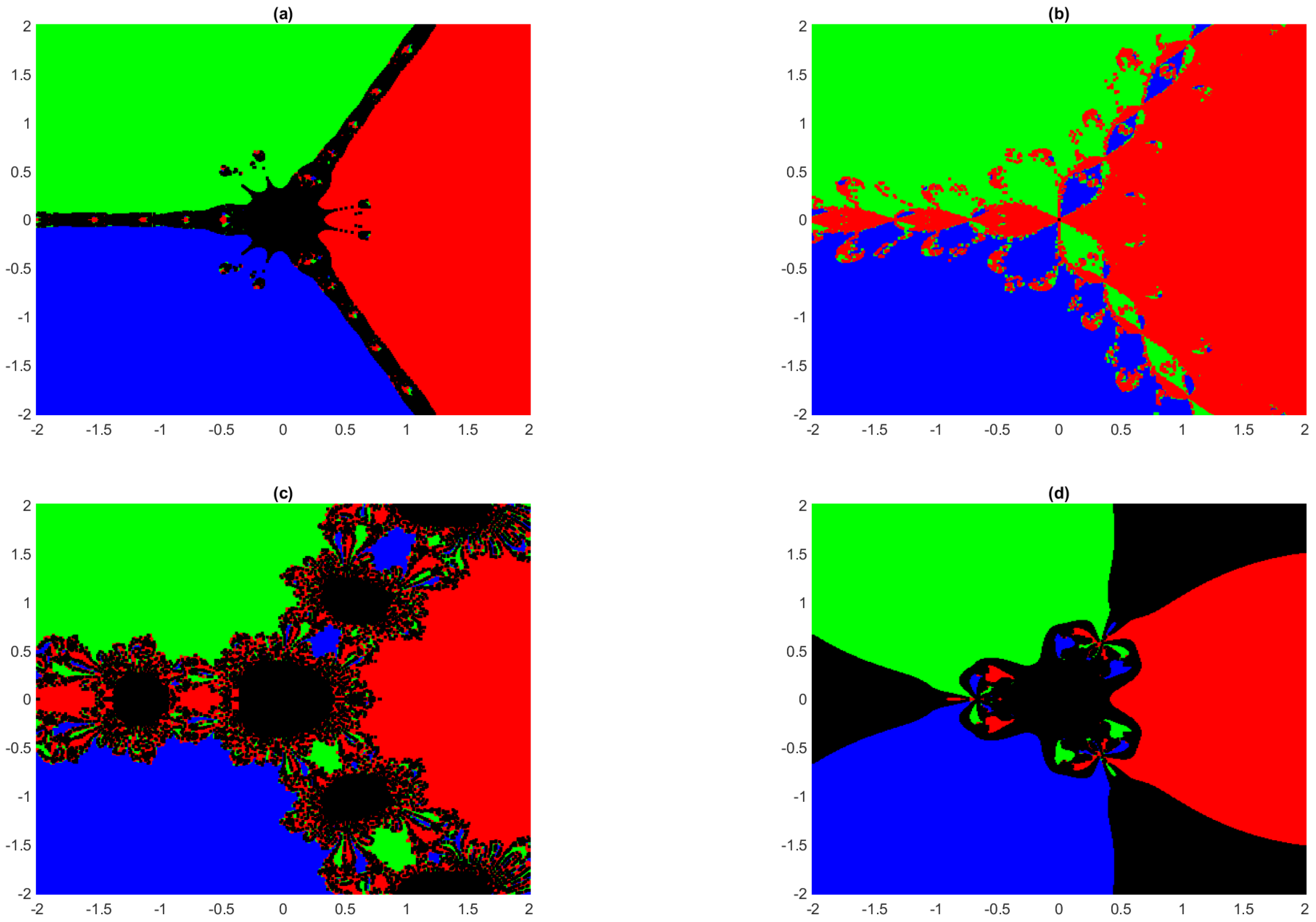
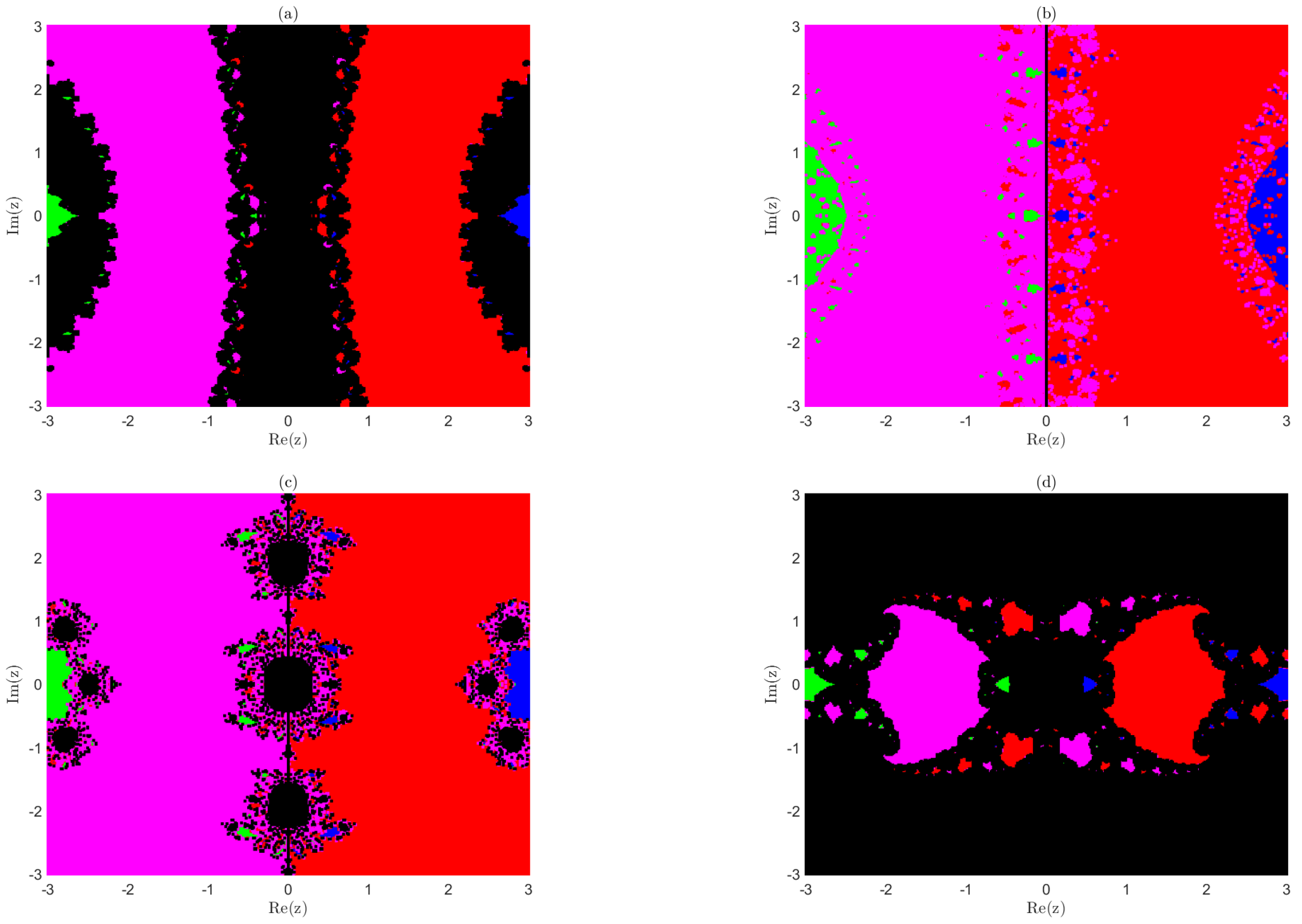
6. Dynamical Concepts

This section discusses concepts related to dynamic studies when applied to the solutions of a nonlinear equation (in both real and complex variable cases). Let G : D D be an iterative map for Equation (1), where D is either R 2 { ( , ) } or C ^ = C { } . A point α D is called an attracting fixed point of G if G ( α ) = α and | G ( α ) | < 1 . A point x 0 is called an initial point or initial guess for the convergence process if the sequence { G k ( x 0 ) } k 0 converges to the solution α of (1). The difficulty lies in making the correct initial guesses. The set
O ( α ) : = x D : { G k ( x ) } k 0 converges to a solution α of Equation ( 1 )
is called the basin of attraction of α . The set of correct initial guesses for the convergence process is precisely the union of all the basins corresponding to solutions of Equation (1). More details on this can be found in [20,21,22,23]. The performance of methods (4) and (5) is investigated in Examples 4 and 5 by considering the following steps:
  • Dividing the region R that contains all the solutions of the equation in 401 × 401 equidistant grid points. The grid points are considered as the initial points for the convergence process.
  • P j denotes the percentage of grid points for which the sequence { G k } k 0 converges to a solution q j , j = 1 , 2 , 3 , 4 of the given equation, and P 0 denotes the percentage of grid points for which the sequence { G k } k 0 does not converge to any of the solutions of the equation given in Examples 4 and 5.
  • To obtain a visual picture, colors blue, green, red, and magenta are assigned to the grid points for which the sequence { G k } k 0 does not converge to q j , j = 1 , 2 , 3 , 4 , respectively, and black is assigned to grid points for which the sequence { G k } k 0 does not converge to any of the solutions of the given equation in Examples 4 and 5.
  • An error tolerance of 10 8 in a maximum of 50 iteration is considered.
We consider the following two earlier studied Jarratt-like sixth-order iterative methods for comparing the performance of the method (5):
Method introduced by Narang et al. in [10]
y k = x k 2 3 Ψ ( x k ) 1 Ψ ( x k ) , A n = I Ψ ( x k ) 1 Ψ ( y k ) z k = x k 1 2 A n I 1 4 A n + 11 8 A n 2 Ψ ( x k ) 1 Ψ ( x k ) x k + 1 = z k I + 3 2 A n Ψ ( x k ) 1 Ψ ( z k ) .
Method introduced by Hueso et al. in [24]
y k = x k 2 3 Ψ ( x k ) 1 Ψ ( x k ) , B n = Ψ ( y k ) 1 Ψ ( x k ) z k = x k 5 8 I + 3 8 B n 2 Ψ ( x k ) 1 Ψ ( x k ) x k + 1 = z k 9 4 I + 11 8 B n 15 8 B n 1 Ψ ( y k ) 1 Ψ ( z k ) .
Example 4.
Consider a system of equations given by
3 s 2 t t 3 = 0 s 3 3 s t 2 = 1 ,
for generating the basin of attractions to the solutions q 1 = 1 2 , 3 2 , q 2 = 1 2 , 3 2 , and q 3 = ( 1 , 0 ) of the system. Here, q 1 , q 2 and q 3 are in R = [ 2 , 2 ] × [ 2 , 2 ] . The basin of attractions of the solutions is given in Figure 2.
Example 5.
Consider a complex polynomial with four distinct real roots:
P ( z ) = z ( z 1 ) ( z 2 ) ( z 3 ) .
The roots of the polynomial P are q 1 = 0 , q 2 = 1 , q 3 = 2 and q 4 = 3 . All the roots belong to the region R = z = x + i y | 3 R e ( z ) 3 , 3 I m ( z ) 3 . The basin of attractions of the solutions is given in Figure 3.
Observation 2.
From Figure 2 and Figure 3, one can observe that the sixth-order extended method (5) of the fourth-order method (4) gives much better convergence results than earlier studied six-order methods (35) and (36). This is evident by the numerical results in Table 2 and Table 3.
All the computations were performed by MATLAB (Version: 24.2.0.2729000 (R2024b)); operating system: Linux 5.15.0-1062-aws #68 20.04.1-Ubuntu SMP, Wed May 1 15:24:09 UTC 2024 x86_64.

7. Conclusions

Conditions ( A 1 ) ( A 7 ) on the operator Ψ are sufficient to demonstrate the semi-local and local convergence analyses of methods (4) and (5), with a calculable radius of convergence ball.
Method (4) is shown to be more applicable than the earlier studies in [13].
The extended method (5) has a better performance in terms of the basin of attractions comparisons than the earlier studied sixth-order methods (35) and (36). Observations in Section 5 and Section 6 support our theoretical findings.
The technique of this study is very general. Therefore, it can be utilized to extend the usage of other methods [10,11,13,14,15,16,17,18,19,20,21,22,23,24]. This will be the focus of future research.

Author Contributions

Conceptualization, validation, formal analysis, investigation, and visualization by I.B., K.S., S.G., I.K.A. and M.I.A. All authors have read and agreed to the published version of the manuscript.

Funding

This research was funded by the Science and Engineering Research Board, Govt. of India, grant number CRG/2021/004776.

Data Availability Statement

Data are contained within the article.

Acknowledgments

Santhosh George thanks the Science and Engineering Research Board, Govt. of India, for providing financial support. Indra Bate would like to thank the National Institute of Technology Karnataka, India, for their support.

Conflicts of Interest

The authors declare no conflicts of interest.

References

  1. Ostrowski, A.M. Solution of Equations and Systems of Equations, 2nd ed.; Pure and Applied Mathematics; Academic Press: New York, NY, USA; London, UK, 1966; Volume 9, pp. xiv+338. [Google Scholar]
  2. Kantorovich, L. Sur la méthode de Newton. Travaux De L’institut Des Mathématiques Steklov 1949, XXVIII, 104–144. [Google Scholar]
  3. Bartle, R.G.; Sherbert, D.R. Introduction to Real Analysis, 4th ed.; John Wiley & Sons, Inc.: New York, NY, USA, 2011; pp. xii+404. [Google Scholar]
  4. Argyros, I.K. Computational Theory of Iterative Methods; Studies in Computational Mathematics; Elsevier B. V.: Amsterdam, The Netherlands, 2007; Volume 15, pp. xvi+487. [Google Scholar]
  5. Ortega, J.M.; Rheinboldt, W.C. Iterative Solution of Nonlinear Equations in Several Variables; Classics in Applied Mathematics; SIAM: Philadelphia, PA, USA, 2000; Volume 30, pp. xxvi+572. [Google Scholar]
  6. Argyros, I.K. Convergence and Applications of Newton-Type Iterations; Springer: New York, NY, USA, 2008; pp. xvi+506. [Google Scholar]
  7. Bruck, R.E.; Reich, S. A general convergence principle in nonlinear functional analysis. Nonlinear Anal. 1980, 4, 939–950. [Google Scholar]
  8. Traub, J.F. Iterative Methods for the Solution of Equations; Prentice-Hall Series in Automatic Computation; Prentice-Hall, Inc.: Englewood Cliffs, NJ, USA, 1964; pp. xviii+310. [Google Scholar]
  9. Jarratt, P. Some fourth order multipoint iterative methods for solving equations. Math. Comput. 1966, 20, 434–437. [Google Scholar] [CrossRef]
  10. Narang, M.; Bhatia, S.; Kanwar, V. New two-parameter Chebyshev-Halley-like family of fourth and sixth-order methods for systems of nonlinear equations. Appl. Math. Comput. 2016, 275, 394–403. [Google Scholar] [CrossRef]
  11. Cordero, A.; Rojas-Hiciano, R.V.; Torregrosa, J.R.; Vassileva, M.P. A highly efficient class of optimal fourth-order methods for solving nonlinear systems. Numer. Algorithms 2024, 95, 1879–1904. [Google Scholar] [CrossRef]
  12. Bate, I.; Senapati, K.; George, S.; Muniyasamy, M.; Chandhini, G. Jarratt-type methods and their convergence analysis without using Taylor expansion. Appl. Math. Comput. 2025, 487, 1–28. [Google Scholar]
  13. Sharma, J.R.; Arora, H. Efficient Jarratt-like methods for solving systems of nonlinear equations. Calcolo 2014, 51, 193–210. [Google Scholar] [CrossRef]
  14. Ezquerro Fernández, J.A.; Hernández Verón, M.A. Newton’s Method: An Updated Approach of Kantorovich’s Theory; Frontiers in Mathematics; Birkhäuser/Springer: Cham, Switzerland, 2017; pp. xii+166. [Google Scholar]
  15. Weerakoon, S.; Fernando, T.G.I. A variant of Newton’s method with accelerated third-order convergence. Appl. Math. Lett. 2000, 13, 87–93. [Google Scholar]
  16. Sakawa, Y. Optimal control of a certain type of linear distributed-parameter systems. IEEE Trans. Autom. Control 1966, 11, 35–41. [Google Scholar] [CrossRef]
  17. Kumar, S.; Sloan, I.H. A new collocation-type method for Hammerstein integral equations. Math. Comput. 1987, 48, 585–593. [Google Scholar] [CrossRef]
  18. Dolph, C.L. Nonlinear integral equations of the Hammerstein type. Trans. Am. Math. Soc. 1949, 66, 289–307. [Google Scholar] [CrossRef]
  19. Hu, S.; Khavanin, M.; Zhuang, W. Integral equations arising in the kinetic theory of gases. J. Appl. Anal. 1989, 34, 261–266. [Google Scholar] [CrossRef]
  20. Amat, S.; Busquier, S.; Plaza, S. Review of some iterative root-finding methods from a dynamical point of view. Sci. Ser. A Math. Sci. (N.S.) 2004, 10, 3–35. [Google Scholar]
  21. Nayak, T.; Pal, S. Symmetry and Dynamics of Chebyshev’s Method. Mediterr. J. Math. 2025, 22, 1–25. [Google Scholar] [CrossRef]
  22. Varona, J.L. Graphic and numerical comparison between iterative methods. Math. Intell. 2002, 24, 37–46. [Google Scholar] [CrossRef]
  23. Campos, B.; Canela, J.; Vindel, P. Dynamics of Newton-like root finding methods. Numer. Algorithms 2023, 93, 1453–1480. [Google Scholar] [CrossRef]
  24. Hueso, J.L.; Martínez, E.; Teruel, C. Convergence, efficiency and dynamics of new fourth and sixth order families of iterative methods for nonlinear systems. J. Comput. Appl. Math. 2015, 275, 412–420. [Google Scholar] [CrossRef]
Figure 1. Solution curve of the boundary value problem (34).
Appliedmath 05 00038 g001
Figure 2. (ad) contain the basin of attractions corresponding to methods (4), (5), (35) and (36), respectively, for Equation (37).
Appliedmath 05 00038 g002
Figure 3. (ad) contain the basin of attractions corresponding to methods (4), (5), (35) and (36), respectively, for Equation (38).
Appliedmath 05 00038 g003
Table 1. Approximations for a solution of the equation given in Example 3 by methods (4) and (5).
Iterations∖Methods(4)(5)
x 1 ( 0.519634152116073 , 0.856463851473843 ) ( 0.367691892458312 , 0.872874907286326 )
x 2 ( 0.143567397874087 , 0.854098376936273 ) ( 0.330887384750105 , 1.289773503139413 )
x 3 ( 0.358769954593253 , 1.250423844938271 ) ( 0.292924940943534 , 1.105736269269610 )
x 4 ( 0.310502308352615 , 1.122370201047817 ) ( 0.290504918408372 , 1.084271081425496 )
x 5 ( 0.292471798020136 , 1.086598145471337 ) ( 0.290514555506250 , 1.084215081491946 )
x 6 ( 0.290529673044637 , 1.084222561605680 ) ( 0.290514555507251 , 1.084215081491351 )
x 7 ( 0.290514555976082 , 1.084215081298624 ) ( 0.290514555507251 , 1.084215081491351 )
x 8 ( 0.290514555507251 , 1.084215081491351 ) ( 0.290514555507251 , 1.084215081491351 )
Table 2. Convergence result of methods (4), (5), (35) and (36) for (37).
Methods P j P 1 P 2 P 3 P 0
(4) 30.3792 30.3792 33.5632 5.6784
(5) 32.3667 32.3667 35.2659 0.0012
(35) 29.4289 29.4289 27.6497 13.4925
(36) 24.7984 24.7984 22.9663 27.4370
Table 3. Convergence result of methods (4), (5), (35) and (36) for (38).
Methods P j P 1 P 2 P 3 P 4 P 0
(4) 1.0752 1.0752 31.4326 31.4326 34.9842
(5) 5.1399 5.1399 44.7354 44.7354 0.2494
(35) 3.7618 3.7618 43.3940 43.3940 5.6884
(36) 1.0497 1.0497 9.8246 9.8246 78.2514
Disclaimer/Publisher’s Note: The statements, opinions and data contained in all publications are solely those of the individual author(s) and contributor(s) and not of MDPI and/or the editor(s). MDPI and/or the editor(s) disclaim responsibility for any injury to people or property resulting from any ideas, methods, instructions or products referred to in the content.

