Mathematical Analysis of a Navier–Stokes Model with a Mittag–Leffler Kernel

Abstract

In this paper, we establish the existence and uniqueness results of the fractional Navier–Stokes (N-S) evolution equation using the Banach fixed-point theorem, where the fractional order $\mathsf{\beta }$ is in the form of the Atangana–Baleanu–Caputo fractional order. The iterative method combined with the Laplace transform and Sumudu transform is employed to find the exact and approximate solutions of the fractional Navier–Stokes equation of a one-dimensional problem of unsteady flow of a viscous fluid in a tube. In the domains of science and engineering, these methods work well for solving a wide range of linear and nonlinear fractional partial differential equations and provide numerical solutions in terms of power series, with terms that are simple to compute and that quickly converge to the exact solution. After obtaining the solutions using these methods, we use Mathematica software Version 13.0.1.0 to present them graphically. We create two- and three-dimensional plots of the obtained solutions at various values of $\mathsf{\beta }$ and manipulate other variables to visualize and model relationships between the variables. We observe that as the fractional order $\mathsf{\beta }$ becomes closer to the integer order 1, the solutions approach the exact solution. Lastly, we plot a 2D graph of the first-, second-, third-, and fourth-term approximations of the series solution $\mathrm{a}\mathrm{n}\mathrm{d}$ observe from the graph that as the number of iterations increases, the approximate solutions become close to the series solution of the fourth-term approximation.

1. Introduction

In this paper, we discuss the existence and the uniqueness of the solution of the time- fractional Navier–Stokes equation of a viscous fluid in unsteady flow through a tube applied to Atangana–Baleanu–Caputo fractional derivative (fractional derivatives without singular kernels). The Navier–Stokes equation is specified as the nonlinear partial differential equation that describes the motion of an incompressible Newtonian fluid and it was named in honor of French engineer Claude-Louis Navier (1785–1836) and English physicist and mathematician Sir George Gabriel Stokes (1819–1903). It is referred to as Newtonian fluid because it was derived using Newton’s second law of motion by considering the forces acting on the fluid elements so that the stress tensor appears in the form of the usual Cauchy momentum equation. This Navier–Stokes equation is the generalization of the equation of motion pioneered by the famous Swiss mathematician Leonhard Euler (1707–1783) to describe the flow of incompressible and frictionless fluids. Navier–Stokes equations are used to model water flow in a pipe, weather forecasting, ocean currents, and airflow around a wing [1]. Furthermore, they assist with the design of cars and aircraft, the study of blood flow, the analysis of pollution, the design of power stations, and a lot of other things. Together with Maxwell’s equations, they may be utilized to model and study magneto-hydrodynamics [1].

The fractional Navier–Stokes equation has been handled by many researchers, such as in [2,3,4,5,6,7,8,9,10]. In [7], the Adomian decomposition method (ADM) was utilized by applying the operator $J^{\alpha }$, the inverse of the operator $D^{\alpha }$, on both sides of the fractional Navier–Stokes equation, where $D^{\alpha }$ is the Caputo time-fractional differential operator of order $\alpha >0$. The Caputo time-fractional Navier–Stokes equation, which describes the motion of a viscous fluid in a tube, has been solved in [4] by combining the Laplace transform with the Adomian decomposition approach. In [2], the Caputo time-fractional Navier–Stokes equation describing the motion of a viscous fluid in a tube was solved using the homotopy perturbation transform method (HPTM). In [3], the Caputo–Fabrizio time-fractional Navier–Stokes equation was solved utilizing the iterative Laplace transform method (ILTM). The existence and uniqueness of the Navier–Stokes equation solutions with fractional time derivatives were examined in [5]. The use of an improved Navier–Stokes (N-S) equation with a fractional derivative to explore the unsteady translational motion of a rigid sphere in an incompressible viscous fluid was handled in [6].

In [2], the Navier–Stokes equation is determined as the essential condition of computational liquid elements, relating pressure and external forces following up on a liquid to the reaction of the liquid stream.

In this study, we model the fractional Navier–Stokes equation. The fractional Navier–Stokes and continuity equation are given as [2]

$$\left\{\begin{array}{l}{}_{ }{}^{CFD}D_t^{\mathsf{\beta }}\mathrm{u}+\left(\mathrm{u}\cdot \nabla \right)\mathrm{u}=-{\displaystyle \frac{1}{\rho }}\nabla \mathrm{p}+\nu {\nabla }^2\mathrm{u},0<\mathsf{\beta }\le 1,t>0,\\ \nabla \cdot \mathrm{u}=0,\end{array}\right.$$

(1)

where $\mathrm{u}$ is the fluid velocity, $\mathrm{p}$ is the fluid pressure, $\nu$ is the fluid viscosity, $\rho$ is the fluid density, ${}_{ }{}^{CFD}D_t^{\mathsf{\beta }}$ is the Caputo fractional derivative, $\nabla$ is the gradient differential operator, and ${\nabla }^2$ is the Laplacian operator. It is important to mention that if the viscosity $\left(\nu \right)$ is set equal to zero, then the Navier–Stokes Equation (1) reduces to Euler’s equation of motion of incompressible and frictionless fluids.

Because our objective is to assess the impact of the Mittag–Leffler kernel on the Navier–Stokes system, we replace ${}_{ }{}^{CFD}D_t^{\mathsf{\beta }}\mathrm{u}$ with ${}_{ }{}^{ABCFD}D_t^{\mathsf{\beta }}\mathrm{u}$ in Equation (1), so that the resulting equation is the fractional Navier–Stokes equation using the Atangana–Baleanu–Caputo derivative. Therefore, we consider the new fractional Navier–Stokes equation in the Atangana–Baleanu–Caputo fractional order and its initial condition as

$$\left\{\begin{array}{l}{}_{ }{}^{ABCFD}D_t^{\mathsf{\beta }}\mathrm{u}+\left(\mathrm{u}\cdot \nabla \right)\mathrm{u}=-{\displaystyle \frac{1}{\rho }}\nabla \mathrm{p}+\nu {\nabla }^2\mathrm{u},0<\mathsf{\beta }\le 1,t>0,\\ \nabla \cdot \mathrm{u}=0.\end{array}\right.$$

(2)

Then, we intend to find the solution using the Laplace or Sumudu transform of the ABCFD coupled with the iterative method (IM) applied to a one-dimensional problem of unsteady flow of a viscous fluid in a tube. The advantage of using this method is that we combine the two methods, namely, the Laplace or Sumudu transform and the iterative method (IM), which are very useful for finding the exact and approximate solutions of linear and nonlinear differential equations; moreover, the method helps avoid many complicated computational tasks compared to the normal technique. Another advantage is that the ABCFD applied in Equation (2) is nonlocal, meaning that when modeling a real physical phenomenon, the state of the system does not only depend on the present time but also the history.

Since Navier–Stokes equations are generally nonlinear partial derivatives, they can be found in almost all real-world scenarios [9]; however, some can be reduced to linear equations in specific situations, such as one-dimensional flow. For instance, fluid flow through a cylindrical tube can be modeled as the initial value problem with cylindrical coordinates as follows (see [2,3,4,9,10]):

$${\displaystyle \frac{{\partial }^{\mathsf{\beta }}\mathrm{u}}{\partial t^{\mathsf{\beta }}}}=-{\displaystyle \frac{1}{\rho }}{\displaystyle \frac{\partial \mathrm{p}}{\partial z}}+\nu \left[{\displaystyle \frac{{\partial }^2\mathrm{u}}{\partial r^2}}+{\displaystyle \frac{1}{r}}{\displaystyle \frac{\partial \mathrm{u}}{\partial r}}\right],$$

(3)

which is subject to the following initial condition

$$\mathrm{u}\left(r,0\right)=g\left(r\right).$$

(4)

Equations (3) and (4) are the linearized form of Equation (2) in cylindrical coordinates. ${\displaystyle \frac{{\partial }^{\mathsf{\beta }}\mathrm{u}}{\partial t^{\mathsf{\beta }}}}={}_a{}^{ABCFD}D_t^{\mathsf{\beta }}u(t)$ is the Atangana–Baleanu fractional derivative, with the Caputo derivative, of the velocity of the fluid $u$ with respect to time t, where z denotes the length of the tube and $r$ is the radius of the tube.

2. Preliminaries

In this section, we recall some definitions and theorems of fractional calculus which are very important for our study.

Definition 1. 

Let  $u\in H^1\left(a, b\right), a<b, \mathsf{\beta }\in [0, 1]$; then, the Atangana–Baleanu fractional derivative, with the Caputo derivative, is given by [11,12,13,14]

$${}_a{}^{ABCFD}D_t^{\mathsf{\beta }}u\left(t\right)={\displaystyle \frac{B\left(\mathsf{\beta }\right)}{\left(1-\mathsf{\beta }\right)}}{\int }_a^t \dot{u}\left(\tau \right)E_{\mathsf{\beta }}\left(-{\displaystyle \frac{\mathsf{\beta }(t-\tau {)}^{\mathsf{\beta }}}{1-\mathsf{\beta }}}\right)d\tau ,$$

(5)

where $B(\mathsf{\beta })$ is a normalization function such that $B\left(0\right)=B\left(1\right)=1$ and $E_{\mathsf{\beta }}$ is the Mittag–Leffler function (MLF) defined as follows [11]:

$$E_{\mathsf{\beta }}\left(\chi \right)=\sum _{k=0}^{\mathrm{\infty }} {\displaystyle \frac{{\chi }^k}{\mathsf{\Gamma }\left(\mathsf{\beta }k+1\right)}},\mathsf{\beta }>0.$$

(6)

Theorem 1. 

The Laplace transform of the ABCFD is specified as follows [11,12,14]:

$$\mathcal{L}\left[{}_0{}^{ABCFD}D_t^{\mathsf{\beta }}u\left(t\right)\right]\left(s\right)={\displaystyle \frac{B\left(\mathsf{\beta }\right)}{1-\mathsf{\beta }}}{\displaystyle \frac{s^{\mathsf{\beta }}\mathcal{L}\left[u\left(t\right)\right]\left(s\right)-s^{\mathsf{\beta }-1}u\left(0\right)}{s^{\mathsf{\beta }}+\frac{\mathsf{\beta }}{1-\mathsf{\beta }}}}.$$

(7)

Definition 2. 

According to Refs. [14,15], the Sumudu transform is obtained over the set of functions

$$A=\left\{u\left(t\right):\exists M,{\eta }_1,{\eta }_2>0,|u(t)|<M{e}^{{\displaystyle \frac{|t|}{{\eta }_i}}}, \mathrm{if} t\in (-1{)}^i\times [0,\mathrm{\infty })\right\}$$

and is given by

$$S\left[u\left(t\right)\right]={\int }_0^{\mathrm{\infty }} u\left(st\right)e^{-t}dt, s\in \left(-{\eta }_1,{\eta }_2\right).$$

Definition 3. 

The Sumudu transform of the ABCFD is defined as follows [14]:

$$S\left({}_{ }{}^{ABCFD}D_t^{\mathsf{\beta }}u\left(t\right)\right)={\displaystyle \frac{B\left(\mathsf{\beta }\right)}{1-\mathsf{\beta }\left(1-s^{\mathsf{\beta }}\right)}}\left(S\left(u\right)-u\left(0\right)\right).$$

(8)

Theorem 2. 

The ABCFD and its fractional integral of a function  $u\left(t\right)$  satisfy the Newton–Leibniz formula:

$$u\left(t\right)-u_o={}_{ }{}^{ABFI}I_t^{\mathsf{\beta }}\left({}_{ }{}^{ABCFD}D_t^{\beta }u\left(t\right)\right),$$

where ${}_{ }{}^{ABFI}I_{ }^{ }$ is the Atangana–Baleanu fractional integral so that we have

$$u(t)=u_o+{\displaystyle \frac{1-\mathsf{\beta }}{B\left(\mathsf{\beta }\right)}}u(t)+{\displaystyle \frac{\mathsf{\beta }}{B\left(\mathsf{\beta }\right)\mathsf{\Gamma }\left(\mathsf{\beta }\right)}}{\int }_0^t (t-\tau {)}^{\mathsf{\beta }-1}u\left(\tau \right)d\tau .$$

(9)

3. Existence and Uniqueness of Nonlinear Fractional Derivatives with Respect to the ABCFD

In this section, we apply Banach’s fixed-point theorem to establish the existence and uniqueness results of the fractional initial value problem and we further show that the results also hold for fractional Navier–Stokes Equation (3) and the initial condition (4).

To continue, we consider the following fractional initial value problem:

$$\left\{\begin{array}{l}{}_{ }{}^{ABCFD}D_t^{\mathsf{\beta }}u\left(t\right)=g\left(t,u\left(t\right)\right),0<\mathsf{\beta }\le 1,t>0,\\ u\left(0\right)=u_o.\end{array}\right.$$

(10)

Theorem 3. 

Let $u\in H^1\left(\mathrm{0,1}\right)$; then, $u$ is a solution to the fractional initial value problem (10), if and only if, it is a solution to the following integral equation:

$$u(t)=u_0+{\displaystyle \frac{1-\mathsf{\beta }}{B\left(\mathsf{\beta }\right)}}g(t,u(t))+{\displaystyle \frac{\mathsf{\beta }}{B\left(\mathsf{\beta }\right)\mathsf{\Gamma }\left(\mathsf{\beta }\right)}}{\int }_0^{\tau } g(\tau ,u(\tau ))(t-\tau {)}^{\mathsf{\beta }-1}d\tau .$$

(11)

Proof of Theorem 3. 

Applying the Atangana–Baleanu fractional integral ${}_{ }{}^{ABFI}I_t^{\beta }$ on both sides of Equation (10) and utilizing the properties of the inverse operator will lead us to Equation (11). □

Theorem 4. 

Consider the fractional initial value problem (10), where  $g(t,u(t\left)\right)$ is a smooth function. If$g(t,u(t\left)\right)$ is the Lipschitz function with Lipschitz constant, where

$${\displaystyle \frac{\left(1-\mathsf{\beta }\right)\mathsf{\Gamma }\left(\mathsf{\beta }\right)+t^{\mathsf{\beta }}}{\mathsf{\Gamma }\left(\mathsf{\beta }\right)B\left(\mathsf{\beta }\right)}}L<1,$$

(12)

then the fractional initial value problem (10) has a unique solution in $H^1\left(\mathrm{0,1}\right)$.

Proof of Theorem 4. 

Define the norm on $[0,1]$ using the equation

$$\parallel u\parallel =\underset{t\in \left[\mathrm{0,1}\right]}{\mathrm{s}\mathrm{u}\mathrm{p}} \left|u\left(t\right)\right|,\forall u\in H^1\left(\mathrm{0,1}\right)$$

and consider the operator $T:H^1(0,1)\to H^1(0,1)$, which is defined by

$$(Tu)(t)=u_0+{\displaystyle \frac{1-\mathsf{\beta }}{B(\mathsf{\beta })}}g(t,u(t))+{\displaystyle \frac{\mathsf{\beta }}{B(\mathsf{\beta })\mathsf{\Gamma }(\mathsf{\beta })}}{\int }_0^{\tau } g(\tau ,u(\tau ))(t-\tau {)}^{\mathsf{\beta }-1}d\tau .$$

□

According to Theorem 3, obtaining a solution to the initial value problem (10) is equivalent to finding a fixed point of $T$. Now, for all $u_1\left(t\right),u_2\left(t\right)\in H^1(0,1)$ and $t\in [0,1]$, we have

$$\begin{array}{ll}\left|T\left(u_1\right)\left(t\right)-T\left(u_2\right)\left(t\right)\right|& =\left|{\displaystyle \frac{1-\mathsf{\beta }}{B(\mathsf{\beta })}}\left(u\left(t,u_1\left(t\right)\right)-u\left(t,u_2\left(t\right)\right)\right)\right.\\ & \left.+{\displaystyle \frac{\mathsf{\beta }}{B(\mathsf{\beta })\mathsf{\Gamma }(\mathsf{\beta })}}{\int }_0^t \left(g\left(\tau ,u_1\left(\tau \right)\right)(t-\tau {)}^{\mathsf{\beta }-1}-g\left(\tau ,u_2\left(\tau \right)\right)(t-\tau {)}^{\mathsf{\beta }-1}\right)d\tau \right|\\ & \le {\displaystyle \frac{1-\mathsf{\beta }}{B(\mathsf{\beta })}}L∥u_1-u_2∥+{\displaystyle \frac{\mathsf{\beta }}{B(\mathsf{\beta })\mathsf{\Gamma }(\mathsf{\beta })}}L∥u_1-u_2∥\left|{\int }_0^t (t-\tau {)}^{\mathsf{\beta }-1}d\tau \right|\\ & ={\displaystyle \frac{1-\mathsf{\beta }}{B\left(\mathsf{\beta }\right)}}L∥u_1-u_2∥+{\displaystyle \frac{\mathsf{\beta }}{B\left(\mathsf{\beta }\right)\mathsf{\Gamma }\left(\mathsf{\beta }\right)}}L∥u_1-u_2∥{\displaystyle \frac{t^{\mathsf{\beta }}}{\mathsf{\beta }}}\\ & \le {\displaystyle \frac{\left(1-\mathsf{\beta }\right)\mathsf{\Gamma }\left(\mathsf{\beta }\right)+t^{\mathsf{\beta }}}{\begin{array}{c}\Gamma \left(\mathsf{\beta }\right)B\left(\mathsf{\beta }\right)\\ \end{array}}}L∥u_1-u_2∥.\end{array}$$

Since ${\displaystyle \frac{(1-\mathsf{\beta })\mathsf{\Gamma }(\mathsf{\beta })+t^{\mathsf{\beta }}}{\mathsf{\Gamma }(\mathsf{\beta })B(\mathsf{\beta })}}L<1$, $T$ is a contraction, and according to Banach’s fixed-point theorem, $T$ has a unique fixed point.

Now, we apply Theorems 3 and 4 to the fractional Navier–Stokes Equation (3). If we replace $g(t,u(t\left)\right)$ in Equation (10) with $-{\displaystyle \frac{1}{\rho }}{\displaystyle \frac{\partial \mathrm{p}}{\partial z}}+\nu \left[{\displaystyle \frac{{\partial }^2\mathrm{u}}{\partial r^2}}+{\displaystyle \frac{1}{r}}{\displaystyle \frac{\partial \mathrm{u}}{\partial r}}\right]$ from the fractional Navier–Stokes Equation (3) and also replace the initial condition $u\left(0\right)=u_0$ with $\mathrm{u}(r,0)=g\left(r\right)$, then, according to Theorems 3 and 4, the fractional Navier–Stokes equation (3) with its initial condition has a unique solution in $H^1(0,1)$.

Remark 1. 

According to Ref. [16], when  $0<\mathsf{\beta }<1$ and   $B(\mathsf{\beta })=1$, we have

$${\displaystyle \frac{(1-\mathsf{\beta })\mathsf{\Gamma }(\mathsf{\beta })+1}{\mathsf{\Gamma }(\mathsf{\beta })B(\mathsf{\beta })}}=1-\mathsf{\beta }+{\displaystyle \frac{1}{\mathsf{\Gamma }\left(\mathsf{\beta }\right)}}\le 1-\mathsf{\beta }+1=2-\mathsf{\beta }\le 2.$$

Thus, if $u$ is the Lipschitz function with a Lipschitz constant $L<{\displaystyle \frac{1}{2}}$, the fractional initial value problem (10) has a unique solution in $H^1(0,1)$ when $0<\mathsf{\beta }<1$.

4. Analysis of the Fractional Navier–Stokes Equation with the ABCFD

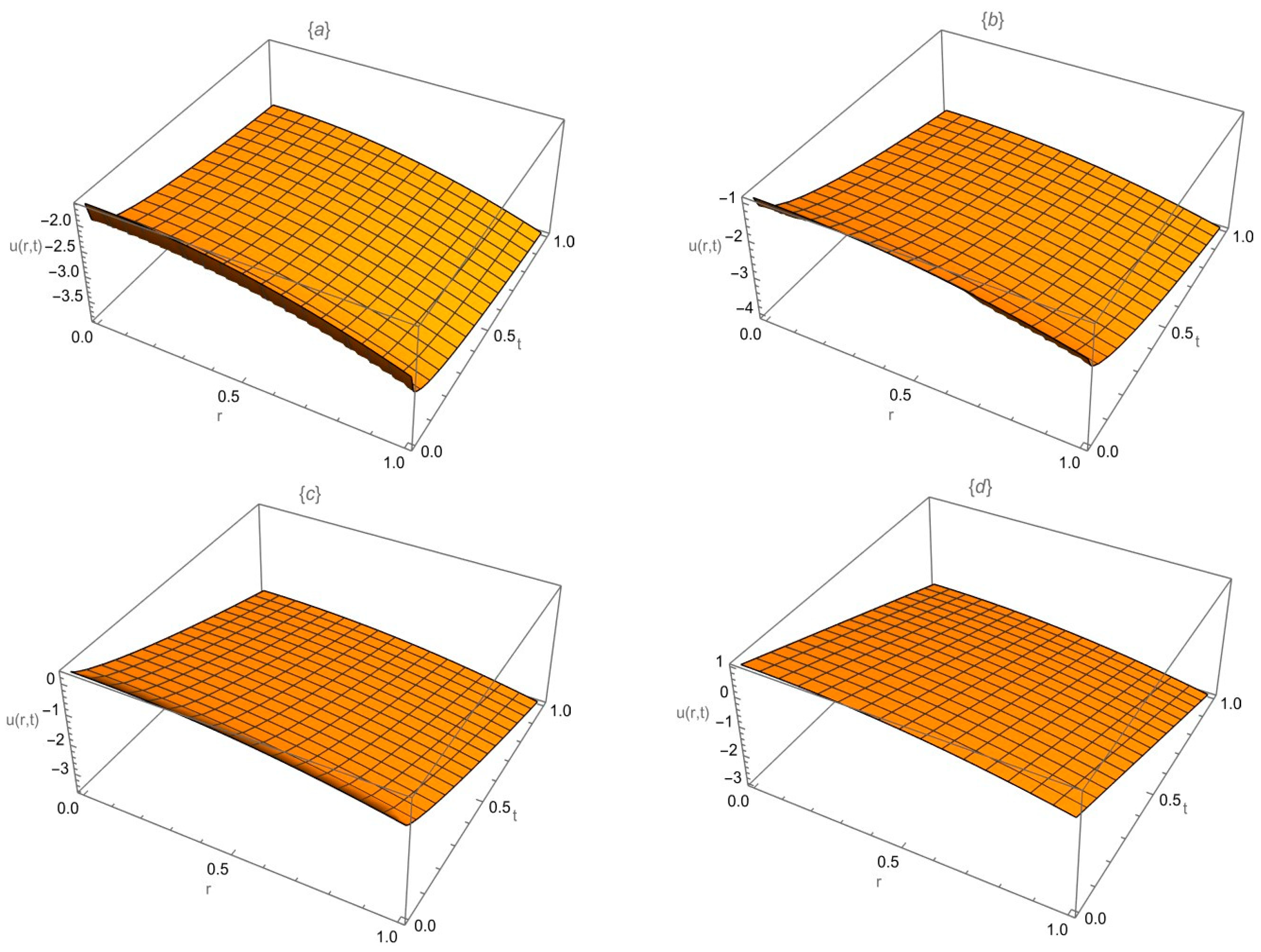
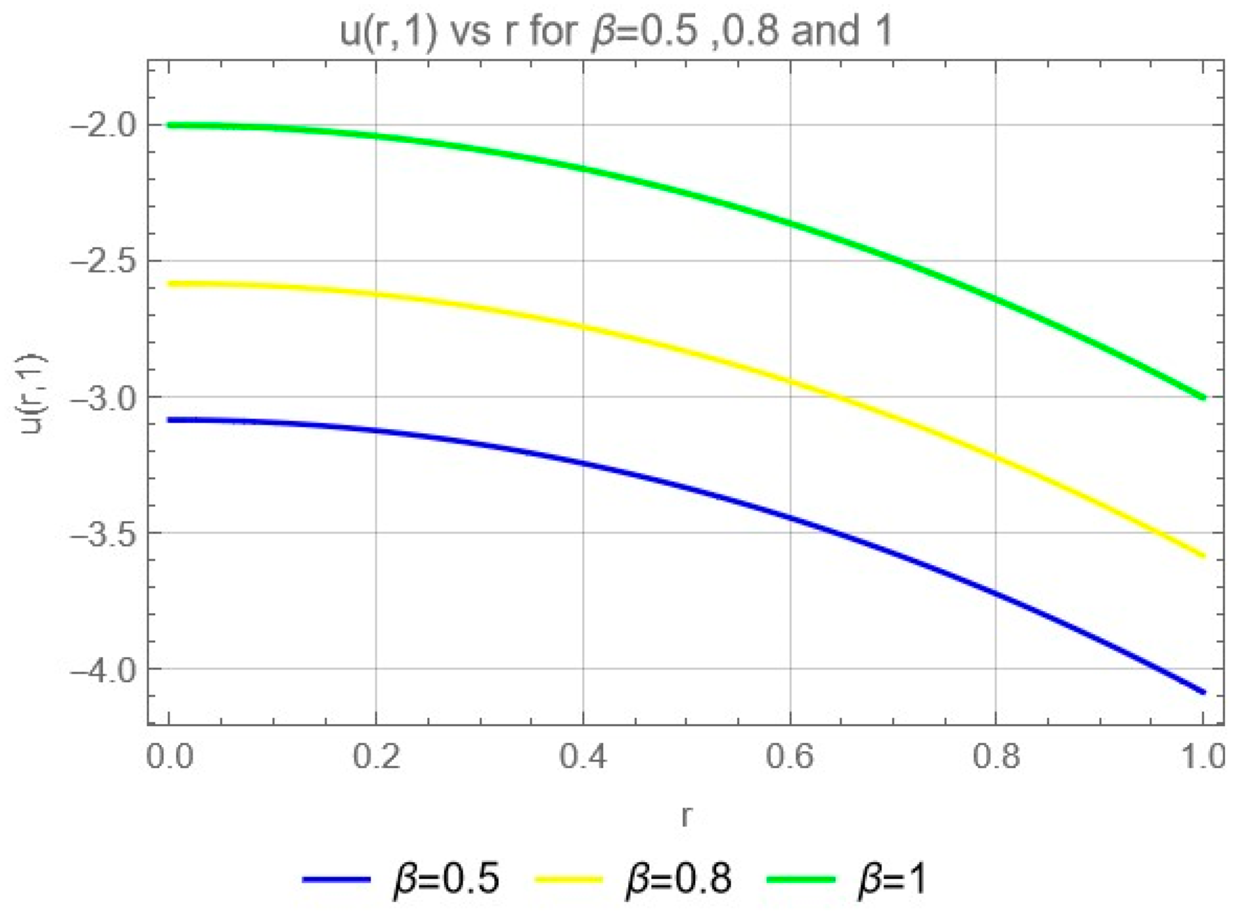
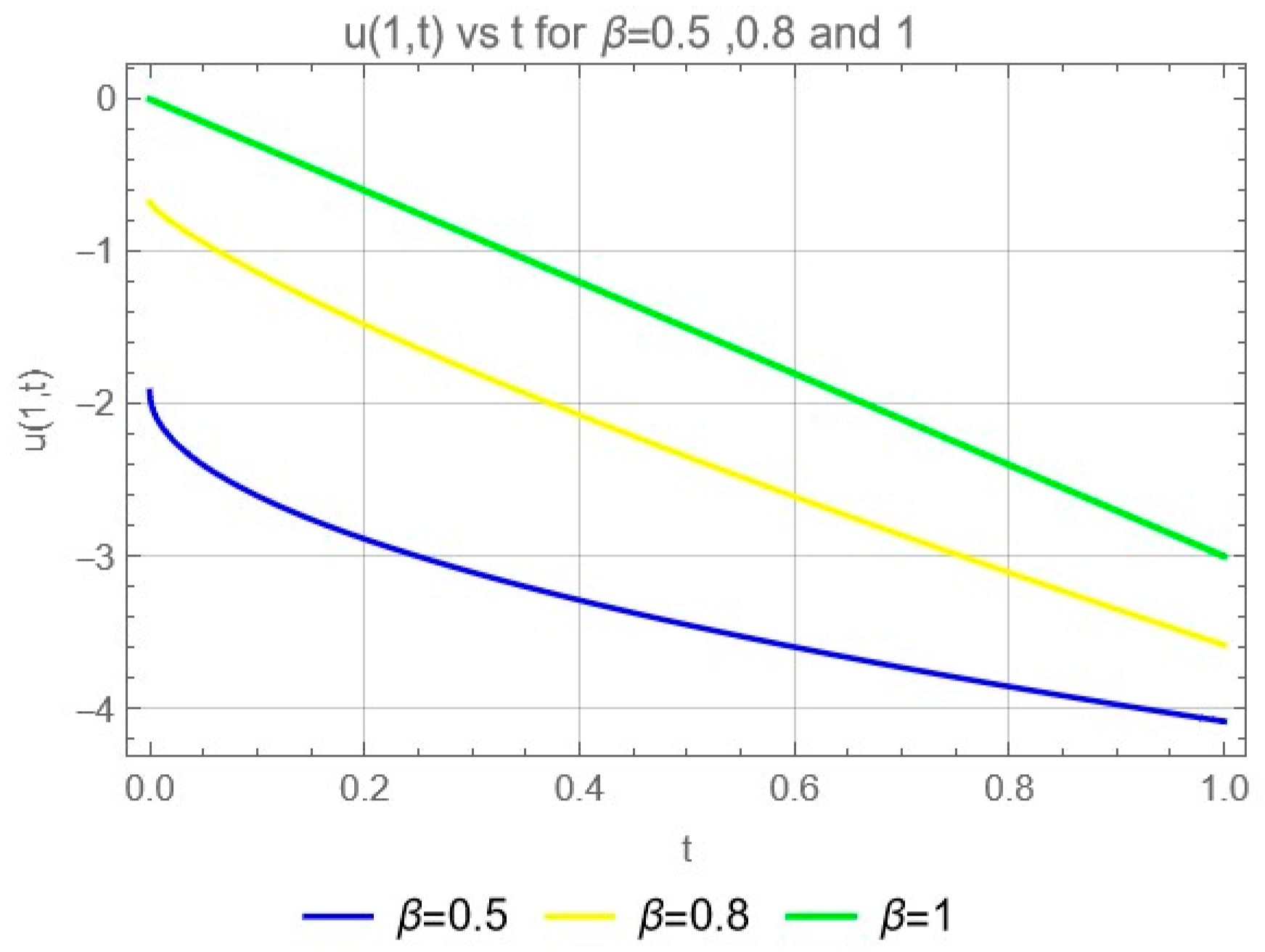
In this section, we consider the Navier–Stokes equation for the one-dimensional motion of a viscous fluid in a tube with an unsteady flow. We solve the fractional Navier–Stokes equation applied to the ABCFD using the iterative Laplace transform method (ILTM).

Consider the following Navier–Stokes equation in cylindrical coordinates:

$${\displaystyle \frac{\partial \mathrm{u}}{\partial t}}=-{\displaystyle \frac{1}{\rho }}{\displaystyle \frac{\partial \mathrm{p}}{\partial z}}+\nu \left[{\displaystyle \frac{{\partial }^2\mathrm{u}}{\partial r^2}}+{\displaystyle \frac{1}{r}}{\displaystyle \frac{\partial \mathrm{u}}{\partial r}}\right],$$

(13)

which is subject to the following initial condition

$$\mathrm{u}\left(r,0\right)=g\left(r\right).$$

(14)

If we apply the fractional derivative of order $\mathsf{\beta }$ in Equation (13) at the extant time derivative term, we obtain

$${\displaystyle \frac{{\partial }^{\mathsf{\beta }}\mathrm{u}}{\partial t^{\mathsf{\beta }}}}=-{\displaystyle \frac{1}{\rho }}{\displaystyle \frac{\partial \mathrm{p}}{\partial z}}+\nu \left[{\displaystyle \frac{{\partial }^2\mathrm{u}}{\partial r^2}}+{\displaystyle \frac{1}{r}}{\displaystyle \frac{\partial \mathrm{u}}{\partial r}}\right],0<\mathsf{\beta }\le 1.$$

(15)

We can write Equation (15) in terms of the Atangana–Baleanu fractional derivative, with the Caputo derivative, as follows:

$${}_{ }{}^{ABCFD}D_t^{\beta }\mathrm{u}=\mathrm{P}+\nu \left[{\displaystyle \frac{{\partial }^2\mathrm{u}}{\partial r^2}}+{\displaystyle \frac{1}{r}}{\displaystyle \frac{\partial \mathrm{u}}{\partial r}}\right],0<\mathsf{\beta }\le 1,$$

(16)

where $\mathrm{P}=-{\displaystyle \frac{1}{\rho }}{\displaystyle \frac{\partial \mathrm{p}}{\partial z}}$.

Applying the Laplace transform (7) on both sides of Equation (16) and using the initial condition (14), we obtain

$$\mathcal{L}\left[{}_{ }{}^{ABCFD}D_t^{\beta }\mathrm{u}\right]=\mathcal{L}\left[\mathrm{P}\right]+\mathcal{L}\left[\nu \left[{\displaystyle \frac{{\partial }^2\mathrm{u}}{\partial r^2}}+{\displaystyle \frac{1}{r}}{\displaystyle \frac{\partial \mathrm{u}}{\partial r}}\right]\right],$$

(17)

$${\displaystyle \frac{B(\mathsf{\beta })}{1-\mathsf{\beta }}}{\displaystyle \frac{s^{\mathsf{\beta }}\mathcal{L}\left[\mathrm{u}\right(r,t\left)\right]\left(s\right)-s^{\mathsf{\beta }-1}u(r,0)}{s^{\mathsf{\beta }}+\frac{\mathsf{\beta }}{1-\mathsf{\beta }}}}=\mathcal{L}\left[\mathrm{P}\right]+\mathcal{L}\left[\nu \left[{\displaystyle \frac{{\partial }^2\mathrm{u}}{\partial r^2}}+{\displaystyle \frac{1}{r}}{\displaystyle \frac{\partial \mathrm{u}}{\partial r}}\right]\right],$$

(18)

$$\mathcal{L}\left[\mathrm{u}\left(r,t\right)\right]={\displaystyle \frac{g\left(r\right)}{s}}+\left[{\displaystyle \frac{\left(1-\mathsf{\beta }\right)}{B\left(\mathsf{\beta }\right)}}+{\displaystyle \frac{\mathsf{\beta }}{B\left(\mathsf{\beta }\right)s^{\mathsf{\beta }}}}\right]\mathcal{L}\left[\mathrm{P}\right]+\left[{\displaystyle \frac{\left(1-\mathsf{\beta }\right)}{B\left(\mathsf{\beta }\right)}}+{\displaystyle \frac{\mathsf{\beta }}{B\left(\mathsf{\beta }\right)s^{\mathsf{\beta }}}}\right]\mathcal{L}\left[\nu \left[{\displaystyle \frac{{\partial }^2\mathrm{u}}{\partial r^2}}+{\displaystyle \frac{1}{r}}{\displaystyle \frac{\partial \mathrm{u}}{\partial r}}\right]\right].$$

(19)

Applying the inverse Laplace transform on both sides of Equation (19), we obtain

$$\mathrm{u}\left(r,t\right)=\mathrm{G}\left(r,t\right)+{\mathcal{L}}^{-1}\left[\left[{\displaystyle \frac{\left(1-\mathsf{\beta }\right)}{B\left(\mathsf{\beta }\right)}}+{\displaystyle \frac{\mathsf{\beta }}{B\left(\mathsf{\beta }\right)s^{\mathsf{\beta }}}}\right]\mathcal{L}\left[\nu \left[{\displaystyle \frac{{\partial }^2\mathrm{u}}{\partial r^2}}+{\displaystyle \frac{1}{r}}{\displaystyle \frac{\partial \mathrm{u}}{\partial r}}\right]\right]\right],$$

(20)

where $\mathrm{G}(r,t)=g(r)+\left[{\displaystyle \frac{(1-\mathsf{\beta })}{B(\mathsf{\beta })}}+{\displaystyle \frac{t^{\mathsf{\beta }}}{B(\mathsf{\beta })\mathsf{\Gamma }(\mathsf{\beta })}}\right]\mathrm{P}$.

The term $\mathrm{G}(r,t)$ represents the term arising from the source term and the given initial conditions. Then, if we apply the iterative method, we obtain the solution as an infinite series:

$$\mathrm{u}\left(r,t\right)=\sum _{k=0}^{\mathrm{\infty }} {\mathrm{u}}_k\left(r,t\right).$$

(21)

Substituting (21) in (20), we obtain

$$\sum _{k=0}^{\mathrm{\infty }} {\mathrm{u}}_k\left(r,t\right)=\mathrm{G}\left(r,t\right)+{\mathcal{L}}^{-1}\left[\left[{\displaystyle \frac{\left(1-\mathsf{\beta }\right)}{B\left(\mathsf{\beta }\right)}}+{\displaystyle \frac{\mathsf{\beta }}{B\left(\mathsf{\beta }\right)s^{\mathsf{\beta }}}}\right]\mathcal{L}\left[\nu \left[{\displaystyle \frac{{\partial }^2}{\partial r^2}}\sum _{k=0}^{\mathrm{\infty }} {\mathrm{u}}_k\left(r,t\right)+{\displaystyle \frac{1}{r}}{\displaystyle \frac{\partial }{\partial r}}\sum _{k=0}^{\mathrm{\infty }} {\mathrm{u}}_k\left(r,t\right)\right]\right]\right].$$

(22)

Comparing the coefficients of ${\mathrm{u}}_k(r,t)$, we obtain

$${\mathrm{u}}_0\left(r,t\right)=\mathrm{G}\left(r,t\right) k=\mathrm{0,1},\mathrm{2,3},4,\dots \dots ,$$

(23)

$${\mathrm{u}}_1\left(r,t\right)={\mathcal{L}}^{-1}\left[\left[{\displaystyle \frac{\left(1-\mathsf{\beta }\right)}{B\left(\mathsf{\beta }\right)}}+{\displaystyle \frac{\mathsf{\beta }}{B\left(\mathsf{\beta }\right)s^{\mathsf{\beta }}}}\right]\mathcal{L}\left[\nu \left[{\displaystyle \frac{{\partial }^2{\mathrm{u}}_0}{\partial r^2}}+{\displaystyle \frac{1}{r}}{\displaystyle \frac{\partial {\mathrm{u}}_0}{\partial r}}\right]\right]\right],$$

(24)

$${\mathrm{u}}_2\left(r,t\right)={\mathcal{L}}^{-1}\left[\left[{\displaystyle \frac{\left(1-\mathsf{\beta }\right)}{B\left(\mathsf{\beta }\right)}}+{\displaystyle \frac{\mathsf{\beta }}{B\left(\mathsf{\beta }\right)s^{\mathsf{\beta }}}}\right]\mathcal{L}\left[\nu \left[{\displaystyle \frac{{\partial }^2{\mathrm{u}}_1}{\partial r^2}}+{\displaystyle \frac{1}{r}}{\displaystyle \frac{\partial {\mathrm{u}}_1}{\partial r}}\right]\right]\right],$$

(25)

$${\mathrm{u}}_3\left(r,t\right)={\mathcal{L}}^{-1}\left[\left[{\displaystyle \frac{\left(1-\mathsf{\beta }\right)}{B\left(\mathsf{\beta }\right)}}+{\displaystyle \frac{\mathsf{\beta }}{B\left(\mathsf{\beta }\right)s^{\mathsf{\beta }}}}\right]\mathcal{L}\left[\nu \left[{\displaystyle \frac{{\partial }^2{\mathrm{u}}_2}{\partial r^2}}+{\displaystyle \frac{1}{r}}{\displaystyle \frac{\partial {\mathrm{u}}_2}{\partial r}}\right]\right]\right],$$

(26)

$${\mathrm{u}}_4\left(r,t\right)={\mathcal{L}}^{-1}\left[\left[{\displaystyle \frac{\left(1-\mathsf{\beta }\right)}{B\left(\mathsf{\beta }\right)}}+{\displaystyle \frac{\mathsf{\beta }}{B\left(\mathsf{\beta }\right)s^{\mathsf{\beta }}}}\right]\mathcal{L}\left[\nu \left[{\displaystyle \frac{{\partial }^2{\mathrm{u}}_3}{\partial r^2}}+{\displaystyle \frac{1}{r}}{\displaystyle \frac{\partial {\mathrm{u}}_3}{\partial r}}\right]\right]\right],$$

(27)

Thus, the series solution of Equation (16) is

$$\mathrm{u}\left(r,t\right)=\sum _{k=0}^{\mathrm{\infty }} {\mathrm{u}}_k\left(r,t\right).$$

(28)

Numerical Examples

We have provided some numerical examples to demonstrate the proficiency and correctness of our solution to the Atangana–Baleanu fractional Navier–Stokes equation, with the Caputo derivative, utilizing the iterative Laplace transform method (ILTM) and iterative Sumudu transform method (ISTM). We have drawn 2D and 3D graphs to analyze the behavior of physical quantities over time as well as other independent variables.

Example 1. 

The time-fractional Navier–Stokes equation concerning the ABCFD when $\nu =1$  is given as

$${}_{ }{}^{ABCFD}D_t^{\beta }\mathrm{u}=\mathrm{P}+{\displaystyle \frac{{\partial }^2\mathrm{u}}{\partial r^2}}+{\displaystyle \frac{1}{r}}{\displaystyle \frac{\partial \mathrm{u}}{\partial r}},0<\mathsf{\beta }\le 1,$$

(29)

which is subject to the following initial condition

$$\mathrm{u}\left(r,0\right)=1-r^2.$$

Applying the Laplace transform (7) on both sides of Equation (29) and using the above initial condition, we obtain

$$\mathcal{L}\left[\mathrm{u}\left(r,t\right)\right]={\displaystyle \frac{1-r^2}{s}}+\left[{\displaystyle \frac{\left(1-\mathsf{\beta }\right)}{B\left(\mathsf{\beta }\right)}}+{\displaystyle \frac{\mathsf{\beta }}{B\left(\mathsf{\beta }\right)s^{\mathsf{\beta }}}}\right]\mathcal{L}\left[\mathrm{P}\right]+\left[{\displaystyle \frac{\left(1-\mathsf{\beta }\right)}{B\left(\mathsf{\beta }\right)}}+{\displaystyle \frac{\mathsf{\beta }}{B\left(\mathsf{\beta }\right)s^{\mathsf{\beta }}}}\right]\mathcal{L}\left[{\displaystyle \frac{{\partial }^2\mathrm{u}}{\partial r^2}}+{\displaystyle \frac{1}{r}}{\displaystyle \frac{\partial \mathrm{u}}{\partial r}}\right].$$

(30)

Applying the Laplace inverse on both sides of Equation (30), we obtain

$$\mathrm{u}\left(r,t\right)=\mathcal{G}\left(r,t\right)+{\mathcal{L}}^{-1}\left[\left[{\displaystyle \frac{\left(1-\mathsf{\beta }\right)}{B\left(\mathsf{\beta }\right)}}+{\displaystyle \frac{\mathsf{\beta }}{B\left(\mathsf{\beta }\right)s^{\mathsf{\beta }}}}\right]\mathcal{L}\left[{\displaystyle \frac{{\partial }^2\mathrm{u}}{\partial r^2}}+{\displaystyle \frac{1}{r}}{\displaystyle \frac{\partial \mathrm{u}}{\partial r}}\right]\right],$$

(31)

where $\mathrm{G}\left(r,t\right)=1-r^2+\left[{\displaystyle \frac{\left(1-\mathsf{\beta }\right)}{B\left(\mathsf{\beta }\right)}}+{\displaystyle \frac{t^{\mathsf{\beta }}}{B\left(\mathsf{\beta }\right)\mathsf{\Gamma }\left(\mathsf{\beta }\right)}}\right]\mathrm{P}.$

$$\mathrm{u}\left(r,t\right)=\sum _{k=0}^{\mathrm{\infty }} {\mathrm{u}}_k\left(r,t\right).$$

(32)

Applying the iterative method coupled with the Laplace transform, we obtain

$$\sum _{k=0}^{\mathrm{\infty }} {\mathrm{u}}_k\left(r,t\right)=\mathrm{G}\left(r,t\right)+{\mathcal{L}}^{-1}\left[\left[{\displaystyle \frac{\left(1-\mathsf{\beta }\right)}{B\left(\mathsf{\beta }\right)}}+{\displaystyle \frac{\mathsf{\beta }}{B\left(\mathsf{\beta }\right)s^{\mathsf{\beta }}}}\right]\mathcal{L}\left[{\displaystyle \frac{{\partial }^2}{\partial r^2}}\sum _{k=0}^{\mathrm{\infty }} {\mathrm{u}}_k\left(r,t\right)+{\displaystyle \frac{1}{r}}{\displaystyle \frac{\partial }{\partial r}}\sum _{k=0}^{\mathrm{\infty }} {\mathrm{u}}_k\left(r,t\right)\right]\right].$$

(33)

Comparing the coefficients of ${\mathrm{u}}_k(r,t)$, we obtain

$$\begin{array}{ll}{\mathrm{u}}_0(r,t)& =1-r^2+\left[{\displaystyle \frac{\left(1-\mathsf{\beta }\right)}{B\left(\mathsf{\beta }\right)}}+{\displaystyle \frac{t^{\mathsf{\beta }}}{B\left(\mathsf{\beta }\right)\mathsf{\Gamma }\left(\mathsf{\beta }\right)}}\right]\mathrm{P}, k=\mathrm{0,1},\mathrm{2,3},4,\dots \dots \dots ,\\ {\mathrm{u}}_1(r,t)=& {\mathcal{L}}^{-1}\left[\left[{\displaystyle \frac{(1-\mathsf{\beta })}{B(\mathsf{\beta })}}+{\displaystyle \frac{\mathsf{\beta }}{B(\mathsf{\beta })s^{\mathsf{\beta }}}}\right]\mathcal{L}\left[{\displaystyle \frac{{\partial }^2{\mathrm{u}}_0}{\partial r^2}}+{\displaystyle \frac{1}{r}}{\displaystyle \frac{\partial {\mathrm{u}}_0}{\partial r}}\right]\right]\\ & =\left(-4\right)\left[{\displaystyle \frac{\left(1-\mathsf{\beta }\right)}{B\left(\mathsf{\beta }\right)}}+{\displaystyle \frac{t^{\mathsf{\beta }}}{B\left(\mathsf{\beta }\right)\mathsf{\Gamma }\left(\mathsf{\beta }\right)}}\right],\\ {\mathrm{u}}_2(r,t)& ={\mathcal{L}}^{-1}\left[\left[{\displaystyle \frac{(1-\mathsf{\beta })}{B(\mathsf{\beta })}}+{\displaystyle \frac{\mathsf{\beta }}{B(\mathsf{\beta })s^{\mathsf{\beta }}}}\right]\mathcal{L}\left[{\displaystyle \frac{{\partial }^2{\mathrm{u}}_1}{\partial r^2}}+{\displaystyle \frac{1}{r}}{\displaystyle \frac{\partial {\mathrm{u}}_1}{\partial r}}\right]\right]\\ & =\left(0\right)\left[\begin{array}{c}{\displaystyle \frac{\left(1-\mathsf{\beta }\right)}{B\left(\mathsf{\beta }\right)}}+{\displaystyle \frac{t^{\mathsf{\beta }}}{B\left(\mathsf{\beta }\right)\mathsf{\Gamma }\left(\mathsf{\beta }\right)}}\\ \end{array}\right],\end{array}$$

so that

$${\mathrm{u}}_k(r,t)=0, \mathrm{for} \mathrm{all} k\ge 2.$$

The series solution of Equation (29) is as follows:

$$\mathrm{u}\left(r,t\right)=\sum _{k=0}^{\mathrm{\infty }} {\mathrm{u}}_k\left(r,t\right)$$

(34)

$$\mathrm{u}\left(r,t\right)=1-r^2+\left(\mathrm{P}-4\right)\left[{\displaystyle \frac{\left(1-\mathsf{\beta }\right)}{B\left(\mathsf{\beta }\right)}}+{\displaystyle \frac{t^{\mathsf{\beta }}}{B\left(\mathsf{\beta }\right)\mathsf{\Gamma }\left(\mathsf{\beta }\right)}}\right].$$

(35)

The method rapidly converges to the exact solution because with fewer iterations, we have achieved a desired accuracy. We can only obtain the exact solution with the third-order term, and if we let $\mathsf{\beta }=1,$ we obtain the classical solution of the normal Navier–Stokes equation as

$$\mathrm{u}\left(r,t\right)=1-r^2+\left(\mathrm{P}-4\right)t.$$

(36)

Figure 1 illustrates the graphical representations of the solution of Equation (29) when $\mathrm{P}=1$ and (a) $\mathsf{\beta }=0.3$, (b) $\mathsf{\beta }=0.5$, (c) $\mathsf{\beta }=0.8,$ or (d) $\mathsf{\beta }=1$.

Figure 2 illustrates the graphical representation for the solution of Equation (29) when $\mathrm{P}=1$, $t=1$, and $\mathsf{\beta }=0.5, \mathsf{\beta }=0.8$, or $\mathsf{\beta }=1$.

Figure 3 illustrates the graphical representation for the solution of Equation (29) when $\mathrm{P}=1$, $r=1$, and $\mathsf{\beta }=0.5,\mathsf{\beta }=0.8,$ or $\mathsf{\beta }=1$.

From the numerical results illustrated in Figure 1, Figure 2 and Figure 3, it is simple to conclude that the solution is continuously dependent on the time-fractional derivative. Figure 1a–d shows the surfaces of the solutions to (29): (a) is for $\mathsf{\beta }=0.3$, (b) is for $\mathsf{\beta }=0.5$, (c) is for $\mathsf{\beta }=0.8,$ and (d) is for $\mathsf{\beta }=1$. It is easy to observe from the surfaces that as the fractional order $\mathsf{\beta }$ approaches an integer order 1, the solutions become closer to the classical exact solution of (29). The same applies to the 2D graphs, shown in Figure 2 and Figure 3. Furthermore, we see from Figure 2 and Figure 3 that the solution u($r,$ $1$) decreases with the increase in the radius of the tube $r$ and u($1,$ $t$) decreases with the increase in time $t$.

Example 2. 

Now, we illustrate how to find the solution of Equation (29) (Example 1), subject to the same initial condition,  $\mathit{u}\left(r,0\right)=1-r^2,$  via the iterative Sumudu transform method (ISTM).

Applying the Sumudu transform (8) on both sides of Equation (29) and using its initial condition, we obtain

$$\mathcal{S}\left[\mathrm{u}\left(r,t\right)\right]=\mathcal{S}\left[1-r^2\right]+\left[{\displaystyle \frac{1-\mathsf{\beta }\left(1-s^{\mathsf{\beta }}\right)}{B\left(\mathsf{\beta }\right)}}\right]\mathcal{S}\left[\mathrm{P}\right]+\left[{\displaystyle \frac{1-\mathsf{\beta }\left(1-s^{\mathsf{\beta }}\right)}{B\left(\mathsf{\beta }\right)}}\right]\mathcal{S}\left[{\displaystyle \frac{{\partial }^2\mathrm{u}}{\partial r^2}}+{\displaystyle \frac{1}{r}}{\displaystyle \frac{\partial \mathrm{u}}{\partial r}}\right],$$

(37)

where $\mathcal{S}$ is the Sumudu transform.

Applying the Sumudu inverse on both sides of Equation (37), we obtain

$$\mathrm{u}\left(r,t\right)=\mathrm{G}\left(r,t\right)+{\mathcal{S}}^{-1}\left[\left[{\displaystyle \frac{1-\mathsf{\beta }\left(1-s^{\mathsf{\beta }}\right)}{B\left(\mathsf{\beta }\right)}}\right]\mathcal{S}\left[{\displaystyle \frac{{\partial }^2\mathrm{u}}{\partial r^2}}+{\displaystyle \frac{1}{r}}{\displaystyle \frac{\partial \mathrm{u}}{\partial r}}\right]\right],$$

(38)

where $\mathrm{G}(r,t)=1-r^2+\left[{\displaystyle \frac{1-\mathsf{\beta }\left[1-\left[\frac{t^{\mathsf{\beta }}}{\mathsf{\Gamma }(\mathsf{\beta }+1)}\right]\right]}{B(\mathsf{\beta })}}\right]\mathrm{P}$.

$$\mathrm{u}\left(r,t\right)=\sum _{k=0}^{\mathrm{\infty }} {\mathrm{u}}_k\left(r,t\right).$$

(39)

Applying the iterative method coupled with the Sumudu transform, we obtain

$$\sum _{k=0}^{\mathrm{\infty }} {\mathrm{u}}_k\left(r,t\right)=\mathrm{G}\left(r,t\right)+{\mathcal{S}}^{-1}\left[\left[{\displaystyle \frac{1-\mathsf{\beta }\left(1-s^{\mathsf{\beta }}\right)}{B\left(\mathsf{\beta }\right)}}\right]\mathcal{S}\left[{\displaystyle \frac{{\partial }^2}{\partial r^2}}\sum _{k=0}^{\mathrm{\infty }} {\mathrm{u}}_k\left(r,t\right)+{\displaystyle \frac{1}{r}}{\displaystyle \frac{\partial }{\partial r}}\sum _{k=0}^{\mathrm{\infty }} {\mathrm{u}}_k\left(r,t\right)\right]\right].$$

(40)

Comparing the coefficients of ${\mathrm{u}}_k(r,t)$, we obtain

$$\begin{array}{ll}{\mathrm{u}}_0(r,t)& =1-r^2+\left[{\displaystyle \frac{1-\mathsf{\beta }\left[1-\left[\frac{t^{\mathsf{\beta }}}{\mathsf{\Gamma }\left(\mathsf{\beta }+1\right)}\right]\right]}{B\left(\mathsf{\beta }\right)}}\right]\mathrm{P}, k=\mathrm{0,1},\mathrm{2,3},4,\dots \dots \dots ,\\ {\mathrm{u}}_1(r,t)& ={\mathcal{S}}^{-1}\left[\left[{\displaystyle \frac{1-\mathsf{\beta }\left(1-s^{\mathsf{\beta }}\right)}{B(\mathsf{\beta })}}\right]\mathcal{S}\left[{\displaystyle \frac{{\partial }^2{\mathrm{u}}_0}{\partial r^2}}+{\displaystyle \frac{1}{r}}{\displaystyle \frac{\partial {\mathrm{u}}_0}{\partial r}}\right]\right]\\ & =-4\left[{\displaystyle \frac{1-\mathsf{\beta }\left[1-\left[\frac{t^{\mathsf{\beta }}}{\mathsf{\Gamma }\left(\mathsf{\beta }+1\right)}\right]\right]}{B\left(\mathsf{\beta }\right)}}\right],\\ {\mathrm{u}}_2(r,t)& ={\mathcal{S}}^{-1}\left[\left[{\displaystyle \frac{1-\mathsf{\beta }\left(1-s^{\mathsf{\beta }}\right)}{B(\mathsf{\beta })}}\right]\mathcal{S}\left[{\displaystyle \frac{{\partial }^2{\mathrm{u}}_1}{\partial r^2}}+{\displaystyle \frac{1}{r}}{\displaystyle \frac{\partial {\mathrm{u}}_1}{\partial r}}\right]\right]\\ & =\left(0\right)\left[{\displaystyle \frac{1-\mathsf{\beta }\left[1-\left[\frac{t^{\mathsf{\beta }}}{\mathsf{\Gamma }\left(\mathsf{\beta }+1\right)}\right]\right]}{B\left(\mathsf{\beta }\right)}}\right],\end{array}$$

so that

$${\mathrm{u}}_k(r,t)=0, \mathrm{for} \mathrm{all} k\ge 2.$$

The series solution of Equation (29) is

$$\mathrm{u}(r,t)=\sum _{k=0}^{\mathrm{\infty }} {\mathrm{u}}_k(r,t)$$

(41)

$$\mathrm{u}\left(r,t\right)=1-r^2+\left(\mathrm{P}-4\right)\left[{\displaystyle \frac{1-\mathsf{\beta }\left[1-\left[\frac{t^{\mathsf{\beta }}}{\mathsf{\Gamma }\left(\mathsf{\beta }+1\right)}\right]\right]}{B\left(\mathsf{\beta }\right)}}\right].$$

(42)

Then, if $\mathsf{\beta }=1,$ we obtain the same classical solution as in Example 1.

Example 3. 

Consider the following time-fractional Navier–Stokes equation with respect to the ABCFD:

$${}_{ }{}^{ABCFD}D_t^{\beta }\mathrm{u}={\displaystyle \frac{{\partial }^2\mathrm{u}}{\partial r^2}}+{\displaystyle \frac{1}{r}}{\displaystyle \frac{\partial \mathrm{u}}{\partial r}},0<\mathsf{\beta }\le 1,$$

(43)

which is subject to the following initial condition

$$\mathrm{u}\left(r,0\right)=r.$$

Applying the Laplace transform (7) on both sides of Equation (43) and using the above initial condition, we obtain

$$\mathcal{L}\left[\mathrm{u}\left(r,t\right)\right]={\displaystyle \frac{r}{s}}+\left[{\displaystyle \frac{\left(1-\mathsf{\beta }\right)}{B\left(\mathsf{\beta }\right)}}+{\displaystyle \frac{\mathsf{\beta }}{B\left(\mathsf{\beta }\right)s^{\mathsf{\beta }}}}\right]\mathcal{L}\left[{\displaystyle \frac{{\partial }^2\mathrm{u}}{\partial r^2}}+{\displaystyle \frac{1}{r}}{\displaystyle \frac{\partial \mathrm{u}}{\partial r}}\right].$$

(44)

Applying the Laplace inverse on both sides of Equation (44), we obtain

$$\mathrm{u}\left(r,t\right)=\mathcal{G}\left(r,t\right)+{\mathcal{L}}^{-1}\left[\left[{\displaystyle \frac{\left(1-\mathsf{\beta }\right)}{B\left(\mathsf{\beta }\right)}}+{\displaystyle \frac{\mathsf{\beta }}{B\left(\mathsf{\beta }\right)s^{\mathsf{\beta }}}}\right]\mathcal{L}\left[{\displaystyle \frac{{\partial }^2\mathrm{u}}{\partial r^2}}+{\displaystyle \frac{1}{r}}{\displaystyle \frac{\partial \mathrm{u}}{\partial r}}\right]\right],$$

(45)

where $\mathrm{G}(r,t)=r$.

$$\mathrm{u}\left(r,t\right)=\sum _{k=0}^{\mathrm{\infty }} {\mathrm{u}}_k\left(r,t\right).$$

(46)

Applying the iterative method combined with the Laplace transform, we obtain

$$\sum _{k=0}^{\mathrm{\infty }} {\mathrm{u}}_k\left(r,t\right)=r+{\mathcal{L}}^{-1}\left[\left[{\displaystyle \frac{\left(1-\mathsf{\beta }\right)}{B\left(\mathsf{\beta }\right)}}+{\displaystyle \frac{\mathsf{\beta }}{B\left(\mathsf{\beta }\right)s^{\mathsf{\beta }}}}\right]\mathcal{L}\left[{\displaystyle \frac{{\partial }^2}{\partial r^2}}\sum _{k=0}^{\mathrm{\infty }} {\mathrm{u}}_k\left(r,t\right)+{\displaystyle \frac{1}{r}}{\displaystyle \frac{\partial }{\partial r}}\sum _{k=0}^{\mathrm{\infty }} {\mathrm{u}}_k\left(r,t\right)\right]\right].$$

(47)

Comparing the coefficients of ${\mathrm{u}}_k(r,t)$, we obtain

$$\begin{array}{ll}{\mathrm{u}}_0(r,t)& =r, k=\mathrm{0,1},\mathrm{2,3},4,\dots \dots \dots .,\\ {\mathrm{u}}_1(r,t)& ={\mathcal{L}}^{-1}\left[\left[{\displaystyle \frac{(1-\mathsf{\beta })}{B(\mathsf{\beta })}}+{\displaystyle \frac{\mathsf{\beta }}{B(\mathsf{\beta })s^{\mathsf{\beta }}}}\right]\mathcal{L}\left[{\displaystyle \frac{{\partial }^2{\mathrm{u}}_0}{\partial r^2}}+{\displaystyle \frac{1}{r}}{\displaystyle \frac{\partial {\mathrm{u}}_0}{\partial r}}\right]\right]\\ & =\left({\displaystyle \frac{1}{r}}\right)\left[{\displaystyle \frac{(1-\mathsf{\beta })}{B(\mathsf{\beta })}}+{\displaystyle \frac{t^{\mathsf{\beta }}}{B(\mathsf{\beta })\mathsf{\Gamma }(\mathsf{\beta })}}\right],\\ {\mathrm{u}}_2(r,t)& ={\mathcal{L}}^{-1}\left[\left[{\displaystyle \frac{(1-\mathsf{\beta })}{B(\mathsf{\beta })}}+{\displaystyle \frac{\mathsf{\beta }}{B(\mathsf{\beta })s^{\mathsf{\beta }}}}\right]\mathcal{L}\left[{\displaystyle \frac{{\partial }^2{\mathrm{u}}_1}{\partial r^2}}+{\displaystyle \frac{1}{r}}{\displaystyle \frac{\partial {\mathrm{u}}_1}{\partial r}}\right]\right]\\ & =\left({\displaystyle \frac{1}{r^3}}\right){\left[{\displaystyle \frac{(1-\mathsf{\beta })}{B(\mathsf{\beta })}}+{\displaystyle \frac{t^{\mathsf{\beta }}}{B(\mathsf{\beta })\mathsf{\Gamma }(\mathsf{\beta })}}\right]}^2,\\ {\mathrm{u}}_3(r,t)& ={\mathcal{L}}^{-1}\left[\left[{\displaystyle \frac{(1-\mathsf{\beta })}{B(\mathsf{\beta })}}+{\displaystyle \frac{\mathsf{\beta }}{B(\mathsf{\beta })s^{\mathsf{\beta }}}}\right]\mathcal{L}\left[{\displaystyle \frac{{\partial }^2{\mathrm{u}}_2}{\partial r^2}}+{\displaystyle \frac{1}{r}}{\displaystyle \frac{\partial {\mathrm{u}}_2}{\partial r}}\right]\right]\\ & =\left({\displaystyle \frac{9}{r^5}}\right){\left[{\displaystyle \frac{(1-\mathsf{\beta })}{B(\mathsf{\beta })}}+{\displaystyle \frac{t^{\mathsf{\beta }}}{B(\mathsf{\beta })\mathsf{\Gamma }(\mathsf{\beta })}}\right]}^3,\\ {\mathrm{u}}_4(r,t)& ={\mathcal{L}}^{-1}\left[\left[{\displaystyle \frac{(1-\mathsf{\beta })}{B(\mathsf{\beta })}}+{\displaystyle \frac{\mathsf{\beta }}{B(\mathsf{\beta })s^{\mathsf{\beta }}}}\right]\mathcal{L}\left[{\displaystyle \frac{{\partial }^2{\mathrm{u}}_3}{\partial r^2}}+{\displaystyle \frac{1}{r}}{\displaystyle \frac{\partial {\mathrm{u}}_3}{\partial r}}\right]\right]\\ & =\left({\displaystyle \frac{225}{r^7}}\right){\left[{\displaystyle \frac{(1-\mathsf{\beta })}{B(\mathsf{\beta })}}+{\displaystyle \frac{t^{\mathsf{\beta }}}{\begin{array}{c}B\left(\mathsf{\beta }\right)\Gamma \left(\mathsf{\beta }\right)\\ \end{array}}}\right]}^4,\end{array}$$

so that the series solution of Equation (43) can be expressed as

$$\mathrm{u}\left(r,t\right)=r+\sum _{k=0}^{\mathrm{\infty }} {\displaystyle \frac{1^2\times 3^2\times \dots \dots \times (2k-3{)}^2}{r^{2k-1}}}{\left[{\displaystyle \frac{\left(1-\mathsf{\beta }\right)}{B\left(\mathsf{\beta }\right)}}+{\displaystyle \frac{t^{\mathsf{\beta }}}{B\left(\mathsf{\beta }\right)\mathsf{\Gamma }\left(\mathsf{\beta }\right)}}\right]}^k.$$

(48)

If we use the gamma function property $\mathsf{\Gamma }(\mathsf{\beta })={\displaystyle \frac{\mathsf{\Gamma }(\mathsf{\beta }+1)}{\mathsf{\beta }}}$, then we can write (48) as

$$\mathrm{u}\left(r,t\right)=r+\sum _{k=0}^{\mathrm{\infty }} {\displaystyle \frac{1^2\times 3^2\times \dots \dots \times (2k-3{)}^2}{r^{2k-1}}}{\left[{\displaystyle \frac{\left(1-\mathsf{\beta }\right)}{B\left(\mathsf{\beta }\right)}}+{\displaystyle \frac{\mathsf{\beta }{t}^{\mathsf{\beta }}}{B\left(\mathsf{\beta }\right)\mathsf{\Gamma }\left(\mathsf{\beta }+1\right)}}\right]}^k.$$

(49)

When $\mathsf{\beta }=1$, we obtain the following solution:

$$\mathrm{u}\left(r,t\right)=r+\sum _{k=0}^{\mathrm{\infty }} {\displaystyle \frac{1^2\times 3^2\times \dots \dots \times (2k-3{)}^2}{r^{2k-1}}}{\displaystyle \frac{t^k}{k!}},$$

(50)

which gives similar results to those obtained in [2,3,4].

The approximate solution for Equation (43) when $k=4$ is given by $\mathrm{u}(r,t)={\mathrm{u}}_0(r,t)+{\mathrm{u}}_1(r,t)+{\mathrm{u}}_2(r,t)+{\mathrm{u}}_3(r,t)+{\mathrm{u}}_4(r,t)$, and the graphical representation is provided in Figure 4.

Figure 4 illustrates the graphical representation for the solution of Equation (43), when $k=4$ and (a) $\mathsf{\beta }=0.3$, (b) $\mathsf{\beta }=0.5$, (c) $\mathsf{\beta }=0.8,$ or (d) $\mathsf{\beta }=1$.

Figure 5 illustrates the two-dimensional graphical representation for the approximate solution of Equation (43), when $k=4,$ $r$ = 1, and $\mathsf{\beta }=0.3$, $0.5, 0.8, \mathrm{o}\mathrm{r} 1.$

Figure 6 illustrates the two-dimensional graphical representation for the approximate solution of Equation (43), when $k=4,$ $t$ = 1, and $\mathsf{\beta }=0.3, 0.5, 0.8, \mathrm{o}\mathrm{r} 1.$

Figure 4a–d show the surfaces of the approximate solutions to Equation (43): (a) is for $\mathsf{\beta }=0.3$, (b) is for $\mathsf{\beta }=0.5$, (c) is for $\mathsf{\beta }=0.8,$ and (d) is for $\mathsf{\beta }=1$. It is easy to observe from the surfaces that as the fractional order $\mathsf{\beta }$ approaches an integer order, the approximate solutions become close to the series solution shown in (50) of the fourth-term approximation. Figure 5 shows the increase in velocity $\mathbf{u}\left(1,\mathrm{t}\right)$ with the increase in time $t.$ Figure 6 shows that as the radius of the tube $r$increases, the velocity $\mathrm{of}\mathrm{the}\mathrm{fluid} \mathbf{u}\left(\mathrm{r},1\right)$ decreases rapidly until it becomes constant.

Figure 7 illustrates the two-dimensional graphical representation for approximate solutions of Equation (43) for different values of k when $\mathsf{\beta }=1 \mathrm{a}\mathrm{n}\mathrm{d} r=1.$

From Figure 7, which shows the 2D graphs of the first-, second-, third-, and fourth-term approximate solutions to Equation (43) when $\mathsf{\beta }=1 \mathrm{a}\mathrm{n}\mathrm{d} r=1$, it is easy to observe that as the number of iterations increases, the approximate solutions become close to the series solution shown in (50) of the fourth-term approximation. This indicates that the accuracy of the solutions can be improved by using higher-order approximate solutions. Furthermore, we observe that the solution u($1,t$) increases faster in the fourth-term approximation than with other terms as time $t$ increases.

Remark 2. 

If we consider the Navier–Stokes equation in Example 1 with the viscosity $\left(\nu \right)=0$, then the fractional Navier–Stokes Equation (29) will reduce to the Euler’s equation for incompressible and frictionless fluids in the form

$${}_{ }{}^{ABCFD}D_t^{\beta }\mathrm{u}=\mathrm{P} 0<\mathsf{\beta }\le 1$$

which is subject to the initial condition

$$\mathrm{u}(r,0)=r$$

so that according to Examples 1 and 2, $G(r,t)$ is the exact solution of the Euler’s equation if $\nu =0$.

5. Conclusions

In this paper, the iterative method was utilized to solve time-fractional Navier–Stokes equations applied to a one-dimensional problem of unsteady flow of a viscous fluid in a tube with set initial conditions. The fractional derivative was specified in terms of the Atangana–Baleanu–Caputo derivative. The method was coupled with the Laplace and Sumudu transform to assist with achieving exact and approximate solutions. The analytical results have been provided in terms of a power series with simple computable terms, and it is observed that the solution found by this method rapidly converges to the exact solution. The results demonstrate that the solution continuously depends on the time-fractional derivative. We also provided the graphical representation of the solutions using Mathematica software. The obtained solutions at different values of parameter $\mathsf{\beta }$were drawn in 2D and 3D and were shown to approach the exact solution as the fractional parameter approached the integer order 1. The approximate solutions at different iterations were drawn in 2D and were shown to approach the series solution when we increased the number of iterations. The iterative method coupled with the Laplace or Sumudu transform is a very powerful and efficient technique that can be used to obtain analytical solutions for various types of fractional linear, nonlinear, and partial differential equations. The findings of this study will undoubtedly lead to future research and open the door to more sophisticated studies, which could develop more efficient and accurate methods for solving fractional nonlinear partial differential equations by, for example, attempting to find approximations for these complex equations by applying the fractional Adomian decomposition Sumudu transform method or the homotopy perturbation Sumudu transform method. These findings can also be extended to modeling complex physical phenomena, such as turbulent flows, anomalous diffusion, porous media flow, and viscoelastic fluids, which classical derivatives struggle to model. In addition, in systems that display both fractal and fractional properties, we can combine fractal and fractional derivatives to model phenomena like anomalous diffusion and complex dynamic behaviors. Looking at the above future research directions, we can attempt to answer questions such as how can existing methods be improved or new methods developed to solve fractional Navier–Stokes equations more efficiently? What are the potential applications of fractional Navier–Stokes equations in modeling real-world phenomena? What are the potential applications of fractional Navier–Stokes equations in engineering and scientific problems? How much better are the solutions of the fractional Navier–Stokes equation compared with those of the classical Navier–Stokes equation in terms of accuracy and computational efficiency?

References

1. Akbar, T.; Zia, Q.M.Z. Some Exact Solutions of Two-Dimensional Navier–Stokes Equations by Generalizing the Local Vorticity. Adv. Mech. Eng. 2019, 11, 168781401983189. [Google Scholar] [CrossRef]
2. Kumar, D.; Singh, J.; Kumar, S. A Fractional Model of Navier–Stokes Equation Arising in Unsteady Flow of a Viscous Fluid. J. Assoc. Arab. Univ. Basic. Appl. Sci. 2015, 17, 14–19. [Google Scholar] [CrossRef]
3. Yadav, L.K.; Agarwal, G.; Kumari, M. Study of Navier-Stokes Equation by Using Iterative Laplace Transform Method (ILTM) Involving Caputo- Fabrizio Fractional Operator. J. Phys. Conf. Ser. 2020, 1706, 012044. [Google Scholar] [CrossRef]
4. Kumar, S.; Kumar, D.; Abbasbandy, S.; Rashidi, M.M. Analytical Solution of Fractional Navier–Stokes Equation by Using Modified Laplace Decomposition Method. Ain Shams Eng. J. 2014, 5, 569–574. [Google Scholar] [CrossRef]
5. Zhou, Y.; Peng, L. On the Time-Fractional Navier–Stokes Equations. Comput. Math. Appl. 2017, 73, 874–891. [Google Scholar] [CrossRef]
6. Ashmawy, E.A. Unsteady Translational Motion of a Slip Sphere in a Viscous Fluid Using the Fractional Navier-Stokes Equation. Eur. Phys. J. Plus 2017, 132, 142. [Google Scholar] [CrossRef]
7. Momani, S.; Odibat, Z. Analytical Solution of a Time-Fractional Navier–Stokes Equation by Adomian Decomposition Method. Appl. Math. Comput. 2006, 177, 488–494. [Google Scholar] [CrossRef]
8. Biazar, J.; Babolian, E.; Kember, G.; Nouri, A.; Islam, R. An Alternate Algorithm for Computing Adomian Polynomials in Special Cases. Appl. Math. Comput. 2003, 138, 523–529. [Google Scholar] [CrossRef]
9. Burqan, A.; El-Ajou, A.; Saadeh, R.; Al-Smadi, M. A New Efficient Technique Using Laplace Transforms and Smooth Expansions to Construct a Series Solution to the Time-Fractional Navier-Stokes Equations. Alex. Eng. J. 2022, 61, 1069–1077. [Google Scholar] [CrossRef]
10. Iqbal, S.; Martínez, F. An Approach for Approximating Analytical Solutions of the Navier-Stokes Time-Fractional Equation Using the Homotopy Perturbation Sumudu Transform’s Strategy. Axioms 2023, 12, 1025. [Google Scholar] [CrossRef]
11. Djennadi, S.; Shawagfeh, N.; Arqub, O.A. Well-Posedness of the Inverse Problem of Time Fractional Heat Equation in the Sense of the Atangana-Baleanu Fractional Approach. Alex. Eng. J. 2020, 59, 2261–2268. [Google Scholar] [CrossRef]
12. Atangana, A.; Baleanu, D. New Fractional Derivatives with Nonlocal and Non-Singular Kernel: Theory and Application to Heat Transfer Model. Therm. Sci 2016, 20, 763–769. [Google Scholar] [CrossRef]
13. Atangana, A.; Owolabi, K.M. New Numerical Approach for Fractional Differential Equations. Math. Model. Nat. Phenom. 2018, 13, 3. [Google Scholar] [CrossRef]
14. Bokhari, A.; Baleanu, D.; Belgacem, R. Application of Shehu Transform to Atangana-Baleanu Derivatives. J. Math. Comput. Sci. 2019, 20, 101–107. [Google Scholar] [CrossRef]
15. Alomari, A.K. Homotopy-Sumudu Transforms for Solving System of Fractional Partial Differential Equations. Adv. Differ. Equ. 2020, 2020, 222. [Google Scholar] [CrossRef]
16. Syam, M.I.; Al-Refai, M. Fractional Differential Equations with Atangana–Baleanu Fractional Derivative: Analysis and Applications. Chaos Solitons Fractals X 2019, 2, 100013. [Google Scholar] [CrossRef]
Figure 1. Exact solution of Equation (29) with the initial condition u ( r , 0 ) = 1 r 2 when β = 0.3 , 0.5 , 0.8 , and 1. (a) is the exact solution when β  = 0.3, (b) is the exact solution when β  = 0.5, (c) is the exact solution when β  = 0.8 and (d) is the classical exact solution when β  = 1.
Appliedmath 04 00066 g001
Figure 2. Solution of Equation (29) when t = 1 and β = 0.5 ,   0.8 , and 1.
Appliedmath 04 00066 g002
Figure 3. Solution of Equation (29) when r = 1 and β = 0.5 , 0.8 , and 1.
Appliedmath 04 00066 g003
Figure 4. Approximate solution of Equation (43) with the initial condition u ( r , 0 ) = r when β = 0.3 , 0.5 , 0.8 , and 1. (a) is the fourth-term approximate solution when β  = 0.3, (b) is the fourth-term approximate solution when β  = 0.5, (c) is the fourth-term approximate solution when β  = 0.8 and (d) is the fourth-term approximate solution when β  = 1.
Appliedmath 04 00066 g004
Figure 5. Approximate solution of Equation (43) with the initial condition u ( r , 0 ) = r when r = 1   a n d   β = 0.3 ,   0.5 ,   0.8 , and 1.
Appliedmath 04 00066 g005
Figure 6. Approximate solution of Equation (43) with the initial condition u(r,0) = r when t = 1 and β = 0.3, 0.5, 0.8, and 1.
Appliedmath 04 00066 g006
Figure 7. Approximate solutions of Equation (43) with the initial condition u ( r , 0 ) = r when   β = 1 , r = 1 , and k = 1, k = 2, k=3, and k = 4.
Appliedmath 04 00066 g007
Disclaimer/Publisher’s Note: The statements, opinions and data contained in all publications are solely those of the individual author(s) and contributor(s) and not of MDPI and/or the editor(s). MDPI and/or the editor(s) disclaim responsibility for any injury to people or property resulting from any ideas, methods, instructions or products referred to in the content.