Chebyshev Pseudospectral Method for Fractional Differential Equations in Non-Overlapping Partitioned Domains

Abstract

Fractional differential operators are inherently non-local, so global methods, such as spectral methods, are well suited for handling these non-local operators. Long-time integration of differential models such as chaotic dynamical systems poses specific challenges and considerations that make multi-domain numerical methods advantageous when dealing with such problems. This study proposes a novel multi-domain pseudospectral method based on the first kind of Chebyshev polynomials and the Gauss–Lobatto quadrature for fractional initial value problems.The proposed technique involves partitioning the problem’s domain into non-overlapping sub-domains, calculating the fractional differential operator in each sub-domain as the sum of the ‘local’ and ‘memory’ parts and deriving the corresponding differentiation matrices to develop the numerical schemes. The linear stability analysis indicates that the numerical scheme is absolutely stable for certain values of arbitrary non-integer order and conditionally stable for others. Numerical examples, ranging from single linear equations to systems of non-linear equations, demonstrate that the multi-domain approach is more appropriate, efficient and accurate than the single-domain scheme, particularly for problems with long-term dynamics.

1. Introduction

Fractional differential equations (FDEs) are gaining significant attention in engineering, science, finance and other fields. Unlike classical differential equations, which are limited to integer-order derivatives, FDEs introduce a higher degree of complexity into differential equations by incorporating arbitrary non-integer-order derivatives. Fractional differential operators can be defined in various ways, with the most common definitions being those involving singular kernels, such as the Riemann–Liouville and Caputo fractional differential operators [1,2]. These definitions rely on integrals with power-law kernels, which can sometimes lead to singularities and complicate numerical approximations. These differential operators with power law kernels are, however, advantageous for developing spectral-based methods using basis functions such as the Chebyshev and Legendre polynomials, as these polynomials can be expressed in power series form. Therefore, the Caputo derivative will be used in the numerical method proposed in this study. In recent years, however, there has been a significant interest in non-singular kernels, which provide an alternative framework for defining fractional operators. Examples include the Caputo–Fabrizio and Atangana–Baleanu fractional operators, which use the exponential and Mittag-Leffler functions as kernels, respectively [3,4]. These non-singular kernels were introduced to broaden the scope and applicability of fractional calculus in various fields. This added complexity allows fractional differential operators to capture the memory effects of a system or describe memory-inherent phenomena. As a result, FDEs offer a more robust framework for modeling the intricate dynamics of complex systems across various scientific disciplines [5,6]. Finding analytical solutions for fractional differential equations (FDEs) is particularly challenging; however, several studies have proposed analytical solutions and methods for FDEs, for instance, Ahmadian and Darvishi [7] derived solitons and traveling wave solutions using the tanh-coth, tan-cot, sech-csch and sec-csc expansion methods for the $(1+1)$-dimensional fractional Biswas–Milovic equation [8]. Kumar et al. [9] proposed a modified Laplace decomposition method, which hybridizes the Laplace transform and Adomian decomposition methods to analyze the fractional Navier–Stokes equation that models the unsteady flow of a Newtonian fluid in a tube. The fractional symmetric regularized long wave equation has been resolved analytically using methods such as the $G^{\prime }/G$ expansion method [10], the $G^{\prime }/G^2$ expansion method [11], the extended complex method [11], the direct algebraic method [12] and the Jacobi elliptic function method [13]. Other analytical methods that have been used for FDEs include the Sumudu transform [14], the Kudryashov method [15] and various semi-analytical techniques such as the exp expansion method [16,17] and the sine-cosine method [18], among others. Numerical methods also play an important role in obtaining accurate solutions for FDEs, and they provide valuable insight into the dynamics of systems described by FDEs [19,20].

Many numerical methods for approximating the solutions of FDEs have been proposed. For example, Hattaf et al. [21] introduced a novel numerical approach for approximating the generalized Hattaf fractional derivative (GHF), which involves a fractional differential operator with a non-singular kernel. The numerical method developed was tested on FDEs with analytical solutions to verify its accuracy by comparing the approximate solutions to the exact solutions. Non-linear FDEs describing the dynamics of HIV infection were also solved to demonstrate the applicability of the method to real-world problems. The predictor–corrector methods (PCMs) for FDEs were proposed by Kumar et al. [22], Jhinga and Daftardar-Gejji [23] and Lee et al. [24]. These studies demonstrated that PCMs solve FDEs faster and drastically reduce computational time. Kumar et al. [25] introduced two computationally efficient numerical techniques based on the mid-point and Heun method for linear and non-linear fractional initial value problems (IVPs). The study concluded that the proposed methods offer significant advantages over the traditional and improved Euler methods.

The non-local nature of fractional differential operators sometimes makes analysis and finding solutions of FDEs herculean tasks [26]. Spectral methods have been a powerful numerical technique for approximating the solutions of FDEs [27,28,29]. Unlike other traditional numerical techniques, spectral-based methods are global and highly accurate, making them efficient for solving differential equations [30]. Numerous studies have leveraged the global nature of spectral-based methods to discretize fractional differential operators and obtain numerical solutions of FDEs [31]. Zayernouri and Karniadakis [32] and Zhao et al. [33] proposed an exponentially convergent Galerkin spectral method for FDEs. Zayernouri and Karniadakis [32] compared the performance of the developed spectral-based method and the established finite difference method (FDM) and concluded that the proposed method performs better than the FDM in terms of convergence rate. Khader and Sweilam [34] used the Legendre pseudospectral method to solve the fractional advection-dispersion equation with the Caputo fractional differential operator. The study analyzed the accuracy of the new discrete fractional differential operator by examining its convergence rate and estimating the maximum possible error, and the results were consistent with existing results from the literature. Stochastic fractional differential equations were solved by Cardone et al. [35] using the spectral collocation method. The method involves obtaining a fully discrete version of the original continuous operator and solving a system of non-linear algebraic equations. Tests on several problems demonstrated that the proposed method was effective for the chosen basis functions and collocation points.

Spectral methods exhibit exponential convergence for differential equations with sufficiently smooth solutions. This high level of accuracy has made spectral methods, particularly the Chebyshev pseudospectral method, a popular choice for solving a variety of fractional differential equations. For instance, Doha [36] used the Chebyshev pseudospectral method to approximate the solutions of fractional multi-term differential equations. Similarly, Sweilam [37] applied this method to numerically solve fractional integro-differential equations. Other studies that have used the Chebyshev pseudospectral method to approximate the solution of fractional differential equations include those of Dabiri [38], Oloniiju et al. [39,40,41], among others. However, this desirable property of spectral convergence can deteriorate with large time domains or non-smooth solutions [42]. The multi-domain approach tackles these challenges by offering an accurate and computationally efficient way to manage potentially non-smooth solutions. It can also improve numerical stability and accuracy by breaking down a problem’s domain, especially time-dependent problems, into smaller sub-domains [43]. Samuel and Motsa [44] described a multi-domain spectral collocation method for solving hyperbolic partial differential equations (PDEs) with a large time domain. The study showed that dividing the computational domain into smaller sub-domains gives accurate results and reduces the computational time. Birem and Klein [45] presented a multi-domain spectral method for the Schrödinger equation. Jung and Olmos-Liceaga [46] introduced a non-conforming and non-overlapping multi-domain spectral method to simulate traveling wave solutions in the reaction-diffusion equations. The method has three key features: high-order accuracy and convergence rate, adaptive mesh and the multi-domain technique. Qin et al. [47] proposed a multi-domain Legendre–Galerkin least square method for linear differential equations with variable coefficients. The study established two key properties of the method: continuity, ensuring consistency and smoothness at the endpoints of each sub-domain, and coercivity, ensuring stability and convergence. Additionally, the study established the optimal error estimate in the $H_1$ norm.

This study explores the Chebyshev pseudospectral method in a multi-domain setting as a novel approach to solving FDEs. Here, the domain of the problem is divided into a finite number of non-overlapping sub-domains. The multi-domain approach for FDEs has been applied to problems in biology [48] and finance [49,50]. Maleki and Kajani [48] used the multi-domain Legendre–Gauss pseudospectral method to approximate solutions for the fractional Volterra population growth model. The study demonstrated the effectiveness of the proposed method in tackling a wide range of integro-differential equations, including those with integer and fractional orders. Bambe Moutsinga et al. [49] developed a spectral-based method for fractional differential equations which models valuation within an affine jump-diffusion framework, chaotic and hyper-chaotic systems and fractional pricing models for cryptocurrencies. The study established that the developed spectral method outperforms the MATLAB numerical packages based on the Euler method. Kharazmi [50] investigated a data-driven approach to solving stochastic fractional partial differential equations (SFPDEs) using multi-domain spectral methods. Zhao et al. [51] proposed a multi-domain spectral collocation method (MDSCM) for solving non-linear FDEs. The MDSCM exhibited a significant advantage over the single-domain spectral methods in achieving high accuracy for differential equations with low-regular solutions. Klein and Stoilov [52] proposed a numerical technique for the fractional Laplacian, based on the Riesz fractional operators, defined on $\mathbb{R}$. The integrands are transformed using the underlying $Z_q$ curve to ensure accurate computation within each sub-interval. The transformed integrals within each sub-interval are then solved using the Clenshaw–Curtis algorithm. Tavassoli Kajani [53] proposed a modified Müntz–Legendre collocation technique on a single domain and in a multi-domain setting for the fractional pantograph equation. Xu and Hesthaven [54] proposed a highly accurate and stable multi-domain spectral method with a penalty method for fractional partial advection and diffusion equations. The study concluded that the proposed scheme’s high accuracy makes it well suited for long-term integration of FDEs. It was also noted that the convergence rate aligns with the theoretical analysis of the scheme.

The present study aims to introduce a novel numerical method, the non-overlapping multi-domain Chebyshev pseudospectral method, based on the first kind of Chebyshev polynomials and the Gauss–Lobatto quadrature for fractional differential equations. The choice of Chebyshev polynomials is due to their orthogonality property with respect to their weight function, which simplifies the projection of the approximate solution onto the polynomial space. Additionally, the computation of Chebyshev-Gauss–Lobatto quadrature weights and nodes is quite straightforward, and this reduces computational overhead compared to other orthogonal polynomials. The proposed method works by decomposing the domain of a fractional differential equation into smaller, non-overlapping sub-domains. The novelty of this study lies in its approach of partitioning the domain of a fractional initial value problem into non-overlapping sub-intervals and projecting the solution of the problem onto the space of Chebyshev orthogonal polynomials of the first kind. This technique involves separating the fractional differential operator into the sum of the ‘local’ and ‘memory’ components within each sub-domain. To demonstrate the versatility and efficiency of the proposed method, stability analysis and numerical experimentation on various types of fractional differential equations are carried out. Numerical error analysis is conducted to demonstrate the advantages of the domain decomposition approach over the single-domain Chebyshev pseudospectral method.

The rest of the article is organized as follows: Section 2 provides certain preliminary definitions which are necessary for developing the numerical schemes; Section 3 is devoted to developing and analyzing the numerical scheme for FDEs using the Chebyshev polynomials on the Gauss–Lobatto quadrature in non-overlapping partitioned domains; Section 4 demonstrates the accuracy and effectiveness of the numerical method by presenting some examples ranging from linear single equations to systems of non-linear equations that require long-term integration; and Section 5 ultimately concludes the study.

2. Preliminaries

This section introduces and defines the basic concepts and fractional operators required to develop the numerical scheme.

Definition  1.

Suppose $u:[a,b]\to \mathbb{R}$ is a continuous function, $\gamma >0$ and the Riemann–Liouville fractional order integral of $u\left(t\right)$ is defined as [55]

$$\begin{array}{c}\hfill { }_a^{RL}{I}_t^{\gamma }u\left(t\right)=\left\{\begin{array}{c}{\displaystyle \frac{1}{\Gamma \left(\gamma \right)}}\left(t^{\gamma -1}\ast u\left(t\right)\right)={\displaystyle \frac{1}{\Gamma \left(\gamma \right)}}\underset{a}{\overset{t}{\int }}{(t-\tau )}^{\gamma -1}u\left(\tau \right)d\tau ,t>0,\gamma >0,\hfill \\ u\left(t\right),\gamma =0,\hfill \end{array}\right.\end{array}$$

(1)

where Γ is the Euler gamma function and $\left(t^{\gamma -1}\ast u\left(t\right)\right)$ is the convolution product of the power function, $t^{\gamma -1}$, and the function $u\left(t\right)$.

Definition 2

(Fractional integral of ${(t-a)}^j$). For the power function ${(t-a)}^j$, the fractional integral is defined as [56]

$$\begin{array}{c}\hfill { }_a^{RL}{I}_t^{\gamma }{(t-a)}^j={\displaystyle \frac{\Gamma (j+1)}{\Gamma (j+\gamma +1)}}{(t-a)}^{j+\gamma }.\end{array}$$

(2)

Definition 3.

The left-sided Caputo fractional differential operator is defined as [55]

$$\begin{array}{c}\hfill { }_a^C{D}_t^{\gamma }u\left(t\right)={\displaystyle \frac{1}{\Gamma (\lceil \gamma \rceil -\gamma )}}\left(t^{\lceil \gamma \rceil -\gamma -1}\ast u^{\lceil \gamma \rceil }\left(t\right)\right)={\displaystyle \frac{1}{\Gamma (\lceil \gamma \rceil -\gamma )}}\underset{a}{\overset{t}{\int }}{(t-\tau )}^{\lceil \gamma \rceil -\gamma -1}{u}^{\lceil \gamma \rceil }\left(\tau \right)d\tau ,\lceil \gamma \rceil -1<\gamma \le \lceil \gamma \rceil ,\end{array}$$

(3)

where $\lceil \gamma \rceil$ is the ceiling of γ, $\lceil \gamma \rceil \ge \gamma$ and ${\displaystyle \left(t^{\lceil \gamma \rceil -\gamma -1}\ast u^{\lceil \gamma \rceil }\left(t\right)\right)}$ is the convolution product of the power function, $t^{\lceil \gamma \rceil -\gamma -1}$, and the $\lceil \gamma \rceil$-th integer-order derivative of the function $u\left(t\right)$.

Definition 4

(Fractional derivative of ${(t-a)}^j$). The fractional derivative of ${(t-a)}^j$ is defined as [56]

$$\begin{array}{c}\hfill { }_a^C{D}_t^{\gamma }{(t-a)}^j=\left\{\begin{array}{cc}0\hfill & j\in {\mathbb{N}}_0,j<\lceil \gamma \rceil \hfill \\ {\displaystyle \frac{\Gamma (j+1)}{\Gamma (j+1-\gamma )}}{(t-a)}^{j-\gamma }\hfill & j\in {\mathbb{N}}_0,j\ge \lceil \gamma \rceil .\hfill \end{array}\right.\end{array}$$

(4)

Definition 5.

The set of collocation points used in this study is that of the Chebyshev–Gauss–Lobatto points defined as ${\displaystyle t_r=-cos\left(\frac{r\pi }{N}\right);r=0\left(1\right)N}$ [57].

3. Numerical Discretization and Analysis via the Pseudospectral Method

This section introduces the numerical discretization of a fractional initial value problem using Chebyshev polynomials of the first kind and the Gauss–Lobatto quadrature. It covers the approximations of the fractional derivative of an arbitrary function, both in a single domain and in partitioned, non-overlapping domains. Firstly, the polynomial approximation of an arbitrary function $u\left(t\right)$, continuous on an interval $[0,h]$, is presented in terms of shifted first-kind Chebyshev polynomials. These polynomials are obtained through the following recurrence formula:

$$\begin{array}{c}\hfill {\Pi }_{h,0}\left(t\right)=1,{\Pi }_{h,1}\left(t\right)={\displaystyle \frac{2t}{h}}-1,{\Pi }_{h,j+1}\left(t\right)=2{\Pi }_{h,1}\left(t\right)·{\Pi }_{h,j}\left(t\right)-{\Pi }_{h,j-1}\left(t\right),j\ge 1.\end{array}$$

(5)

The function $u\left(t\right)$ is represented as follows:

$$\begin{array}{c}\hfill u\left(t\right)\approxeq U_h\left(t\right)=\sum _{j=0}^{\infty }{\widehat{u}}_j{\Pi }_{h,j}\left(t\right),t\in [0,h],\end{array}$$

(6)

where the coefficients ${\widehat{u}}_j$ in Equation (6) satisfy the ${\mathcal{l}}^2$ orthogonality condition of the shifted first-kind Chebyshev polynomials, which are defined with respect to the inner product

$$\begin{array}{c}\hfill {\widehat{u}}_j=⟨U_h\left(t\right),{\Pi }_{h,j}\left(t\right)⟩={\displaystyle \frac{1}{{\nu }_j}}{\int }_0^h{\displaystyle \frac{U_h\left(t\right){\Pi }_{h,j}\left(t\right)}{\sqrt{ht-t^2}}}dt={\displaystyle \frac{1}{{\nu }_j}}\sum _{i=0}^{\infty }{U}_h\left(t_i\right){\Pi }_{h,j}\left(t_i\right){\varrho }_i,\end{array}$$

(7)

where

$$\begin{array}{c}\hfill {\nu }_j=\left\{\begin{array}{c}\pi j=0\hfill \\ {\displaystyle \frac{\pi }{2}}\mathrm{otherwise}.\hfill \end{array}\right.\end{array}$$

(8)

If a truncated N-th order approximation of the function is considered and collocated at $N+1$ distinct Chebyshev–Gauss–Lobatto (CGL) points, with $t_r\in [0,h];r=0\left(1\right)N$, then

$$\begin{array}{c}\hfill u\left(t\right)\approxeq \sum _{i=0}^N{U}_h\left(t_i\right){\varrho }_i\sum _{j=0}^N{\displaystyle \frac{1}{{\nu }_j}}{\Pi }_{h,j}\left(t_i\right){\Pi }_{h,j}\left(t_r\right),r=0\left(1\right)N,\end{array}$$

(9)

where ${\varrho }_i$ is the Christoffel number associated with the Chebyshev–Gauss–Lobatto quadrature and is defined as follows:

$$\begin{array}{c}\hfill {\varrho }_i=\left\{\begin{array}{c}{\displaystyle \frac{\pi }{2N}}I=0,N\hfill \\ {\displaystyle \frac{\pi }{N}}\mathrm{otherwise}.\hfill \end{array}\right.\end{array}$$

(10)

Using the following matrix representations

$$\begin{array}{c}\hfill \mathit{\rho }=\left[\begin{array}{cccc}{\varrho }_0& & & \\ & {\varrho }_1& & \\ & & \ddots & \\ & & & {\varrho }_N\end{array}\right],\mathbf{\vartheta }=\left[\begin{array}{cccc}{\displaystyle \frac{1}{{\nu }_0}}& & & \\ & {\displaystyle \frac{1}{{\nu }_1}}& & \\ & & \ddots & \\ & & & {\displaystyle \frac{1}{{\nu }_N}}\end{array}\right],{\mathbf{\Pi }}_h=\left[\begin{array}{cccc}{\Pi }_{h,0}\left(t_0\right)& {\Pi }_{h,0}\left(t_1\right)& \cdots & {\Pi }_{h,0}\left(t_N\right)\\ {\Pi }_{h,1}\left(t_0\right)& {\Pi }_{h,1}\left(t_1\right)& \cdots & {\Pi }_{h,1}\left(t_N\right)\\ ⋮& ⋮& \ddots & ⋮\\ {\Pi }_{h,N}\left(t_0\right)& {\Pi }_{h,N}\left(t_1\right)& \cdots & {\Pi }_{h,N}\left(t_N\right)\end{array}\right],\end{array}$$

(11)

Equation (9) can be expressed as

$$\begin{array}{c}\hfill u\left(t\right)\approxeq \sum _{i=0}^N{U}_h\left(t\right)E_i\left(t_r\right)={\mathbf{E}}^{\mathsf{T}}{\mathbf{U}}_h,\end{array}$$

(12)

where $\mathbf{E}=\mathit{\rho }{\Pi }_h^{\mathsf{T}}\mathbf{\vartheta }{\Pi }_h$ and ${\mathbf{U}}_h={[U_h\left(t_0\right)U_h\left(t_1\right)\dots U_h\left(t_N\right)]}^{\mathsf{T}}$.

3.1. The Discretization of the Fractional Differential Operator in a Single Domain

Now, let us approximate the arbitrary non-integer order of the function $u\left(t\right)$. Assuming that $u\left(t\right)\in {\mathcal{C}}^p\left([0,h]\right)$, where $p\ge N+\lceil \gamma \rceil +1$, representing the space of continuously differentiable functions, $t>0$ and $\gamma >0$, then the approximation for the arbitrary non-integer derivative of $u\left(t\right)$ is given by

$$\begin{array}{c}\hfill { }_0^C{D}_t^{\gamma }u\left(t\right)\approxeq \sum _{i=0}^N{U}_h\left(t_i\right){\varrho }_i\sum _{j=0}^N{\displaystyle \frac{1}{{\nu }_j}}{\Pi }_{h,j}\left(t_i\right){ }_0^C{D}_t^{\gamma }{\Pi }_{h,j}\left(t\right).\end{array}$$

(13)

The fractional-order derivative of the Chebyshev polynomial ${ }_0^C{D}_t^{\gamma }{\Pi }_{h,j}\left(t\right)$ is obtained by using the series form of the polynomial [56], as follows:

$$\begin{array}{c}\hfill { }_0^C{D}_t^{\gamma }{\Pi }_{h,j}\left(t\right)=j\sum _{k=0}^j{\displaystyle \frac{{(-1)}^{j-k}(j+k-1)!2^{2k}}{(j-k)!\left(2k\right)!h^k}}{ }_0^C{D}_t^{\gamma }{t}^k=j\sum _{k=\lceil \gamma \rceil }^j{\displaystyle \frac{{(-1)}^{j-k}(j+k-1)!2^{2k}}{(j-k)!\left(2k\right)!h^k}}{\displaystyle \frac{\Gamma (k+1)}{\Gamma (k-\gamma +1)}}{t}^{k-\gamma }.\end{array}$$

(14)

Proceeding to approximate $t^{k-\gamma }$ as a linear combination of shifted first-kind Chebyshev polynomials at the CGL points, Equation (14) can now be expressed as [39]:

$$\begin{array}{c}\hfill { }_0^C{D}_t^{\gamma }{\Pi }_{h,j}\left(t\right){\approxeq }_h{\mathcal{D}}^{\left(\gamma \right)}{\Pi }_h,\end{array}$$

(15)

where ${ }_h{\mathcal{D}}^{\left(\gamma \right)}=\Delta \Omega \Phi {\Delta }^{\mathsf{T}}\mathbf{\vartheta }$ and $\Delta ,\Omega$ and $\Phi$ are matrices whose entries are defined as follows:

$$\left.\begin{array}{cc}\hfill & {\Delta }_{j,k}=\left\{\begin{array}{cc}1\hfill & j=0,k=0\hfill \\ {\displaystyle \frac{j{(-1)}^{j-k}(j+k-1)!2^{2j}}{(j-k)!\left(2k\right)!h^k}}\hfill & j=1\left(1\right)N,k=0\left(1\right)j\hfill \\ 0\hfill & \mathrm{otherwise}\hfill \end{array}\right.,{\Omega }_{k,k}=\left\{\begin{array}{cc}0\hfill & k<\lceil \gamma \rceil \hfill \\ {\displaystyle \frac{\Gamma (k+1)}{\Gamma (k-\gamma +1)}}\hfill & k=\lceil \gamma \rceil \left(1\right)N\hfill \end{array}\right.,\hfill \\ \hfill & {\Phi }_{p,k}=\left\{\begin{array}{cc}0\hfill & k<\lceil \gamma \rceil \hfill \\ {\displaystyle \frac{\sqrt{\pi }{h}^{k-\gamma +p}\Gamma (k-\gamma +p+\frac{1}{2})}{\Gamma (k-\gamma +p+1)}}\hfill & k=\lceil \gamma \rceil \left(1\right)N,p=0\left(1\right)s,s=0\left(1\right)N.\hfill \end{array}\right.\hfill \end{array}\right\}$$

(16)

Therefore, ${ }_0^C{D}_t^{\gamma }u\left(t\right)$ is now approximated as

$$\begin{array}{c}\hfill { }_0^C{D}_t^{\gamma }u\left(t\right)\approxeq {\left({ }_{0,h}{\mathbf{D}}^{\gamma }\right)}^{\mathsf{T}}{\mathbf{U}}_h,\end{array}$$

(17)

where ${ }_{0,h}{\mathbf{D}}^{\gamma }=\mathit{\rho }{\Pi }_h^{\mathsf{T}}\mathbf{\vartheta }{ }_h{\mathcal{D}}^{\left(\gamma \right)}{\Pi }_h$. We refer to ${\left({ }_{0,h}{\mathbf{D}}^{\gamma }\right)}^{\mathsf{T}}$ as the fractional differentiation matrix in the domain $[0,h]$.

3.2. Discretization of Fractional Differential Operator in Non-Overlapping Partitioned Domains

Assume that $u\left(t\right)$ is defined in $t\in [0,T]$, partitioned into q non-overlapping sub-intervals, such that $0=t_0<t_1<\dots <t_q=T$ and $h_l=t_l-t_{l-1},l=1\left(1\right)q$. Suppose $t\in [t_l,t_{l+1}]$ and $\lceil \gamma \rceil -1<\gamma \le \lceil \gamma \rceil$; then,

$$\left.\begin{array}{cc}\hfill { }_0^C{D}_t^{\gamma }u\left(t\right)& ={\displaystyle \frac{1}{\Gamma (\lceil \gamma \rceil -\gamma )}}{\int }_0^t{(t-\tau )}^{\lceil \gamma \rceil -\gamma -1}{u}^{\lceil \gamma \rceil }\left(\tau \right)d\tau \hfill \\ \hfill & =\sum _{e=1}^l\left[{ }_{t_{e-1}}^C{D}_{t_e}^{\gamma }u\left(t\right)\right]+{ }_{t_l}^C{D}_t^{\gamma }u\left(t\right)\hfill \\ \hfill & =\sum _{e=1}^l\left[{\displaystyle \frac{1}{\Gamma (\lceil \gamma \rceil -\gamma )}}{\int }_{t_{e-1}}^{t_e}{(t-\tau )}^{\lceil \gamma \rceil -\gamma -1}{u}^{\lceil \gamma \rceil }\left(\tau \right)d\tau \right]+{\displaystyle \frac{1}{\Gamma (\lceil \gamma \rceil -\gamma )}}{\int }_{t_l}^t{(t-\tau )}^{\lceil \gamma \rceil -\gamma -1}{u}^{\lceil \gamma \rceil }\left(\tau \right)d\tau .\hfill \end{array}\right\}$$

(18)

The first term in Equation (18) is the ‘memory’, and the latter term of the equation is the local arbitrary-order derivative of $u\left(t\right)$ with respect to $t\in [t_l,t_{l+1}]$. The arbitrary-order derivative in the first sub-domain is local and calculated with no memory term. The two terms in Equation (18) are approximated separately. If the length, $h_l$, of each sub-domain, $[t_l,t_{l+1}]$, is equivalent to h (from discretization in a single domain) in Section 3.1, and we collocate at $N+1$ distinct CGL points, $t_r^l\in [t_l,t_{l+1}]$, with $t_N^l\equiv t_0^{l+1}$, then the second term in Equation (18) is approximated as follows:

$$\begin{array}{c}\hfill { }_{t_l}^C{D}_t^{\gamma }u\left(t\right)\approxeq {\left({ }_{t_l,h_l}{\mathbf{D}}_l^{\gamma }\right)}^{\mathsf{T}}{\mathbf{U}}_{h_l,l},t\in [t_l,t_{l+1}].\end{array}$$

(19)

The first term in Equation (18), the ‘memory’, which is the arbitrary non-integer-order derivative, ${ }_{t_{e-1}}^C{D}_{t_e}^{\gamma }u\left(t\right)$, is approximated as

$$\begin{array}{c}\hfill { }_{t_{e-1}}^C{D}_{t_e}^{\gamma }u\left(t\right)\approxeq \sum _{i=0}^N{U}_h\left(t_i^e\right){\varrho }_i\sum _{j=0}^N{\Pi }_{h_l,j}\left(t_i^e\right){ }_{t_{e-1}}^C{D}_{t_e}^{\gamma }{\Pi }_{h_l,j}\left(t\right),t_i^e\in [t_{e-1},t_e].\end{array}$$

(20)

The derivative ${\displaystyle { }_{t_{e-1}}^C{D}_{t_e}^{\gamma }{\Pi }_{h_l,j}\left(t\right)}$ at the CGL points $t_r^l$ is approximated as ${\displaystyle { }_{t_{e-1}}^C{D}_{t_e}^{\gamma }{\Pi }_{h_l,j}\left(t_r^l\right)\approxeq \Delta \Theta }$, where the entries of $\Theta$ are defined as

$$\begin{array}{c}\hfill {\Theta }_{j,r}=\left\{\begin{array}{cc}{\displaystyle 0}\hfill & j<\lceil \gamma \rceil \hfill \\ {\displaystyle \frac{j!}{\Gamma (\lceil \gamma \rceil -\gamma )(j-\lceil \gamma \rceil )!}}{\int }_{t_{e-1}}^{t_e}{(t_r^l-\tau )}^{\lceil \gamma \rceil -1-\gamma }{(\tau -t_{e-1})}^{j-\lceil \gamma \rceil }d\tau ,\hfill & \begin{array}{c}{t}_r^l\in [t_l,t_{l+1}]\\ j=\lceil \gamma \rceil \left(1\right)N,r=0\left(1\right)N.\end{array}\hfill \end{array}\right.\end{array}$$

(21)

The integral in Equation (21) can be computed using any quadrature formula, such as Newton–Cotes or Gaussian quadrature formulas. Therefore, the first term of Equation (18) is then calculated as

$$\begin{array}{c}\hfill \sum _{e=1}^l{ }_{t_{e-1}}^C{D}_{t_e}^{\gamma }u\left(t\right)\approxeq \sum _{e=1}^l{\left({ }_{t_{e-1},t_e}{\mathbf{D}}_e^{\gamma }\right)}^{\mathsf{T}}{\mathbf{U}}_{h_l,e},\end{array}$$

(22)

where ${\mathbf{U}}_{h_l,e}={[U_{h_l}\left(t_0^e\right)U_{h_l}\left(t_1^e\right)\dots U_{h_l}\left(t_N^e\right)]}^{\mathsf{T}}$, $t_i^e$ are the CGL points mapped onto $[t_{e-1},t_e]$ and ${ }_{t_{e-1},t_e}{\mathbf{D}}_e^{\gamma }=\mathit{\rho }{\Pi }_{h_l}^{\mathsf{T}}\mathbf{\vartheta }\Delta \Theta$.

3.3. Pseudospectral Discretization of FIVPs in Non-Overlapping Partitioned Domain

Consider the fractional initial value problem (FIVP)

$$\left\{\begin{array}{cc}\hfill & { }_0^C{D}_t^{\gamma }u\left(t\right)=\kappa u\left(t\right)+f\left(t\right),t\in (0,T],\hfill \\ \hfill & u\left(0\right)=u_0,\hfill \end{array}\right.$$

(23)

where $\kappa \in \mathbb{C}$ and $\gamma \in (0,1)$. Suppose the domain $[0,T]$ is partitioned into q non-overlapping domains, such that $0=t_0<t_1<t_2<\dots <t_q=T$, and as before, we define $h_l=t_l-t_{l-1}$, $l=1\left(1\right)q$. To obtain the solution of Equation (23) on an arbitrary domain $[t_l,t_{l+1}]$, we rewrite the equation as

$$\left\{\begin{array}{cc}\hfill & \sum _{e=1}^l{ }_{t_{e-1}}^C{D}_{t_e}^{\gamma }u\left(t\right)+{ }_{t_l}^C{D}_t^{\gamma }u\left(t\right)=\kappa u\left(t\right)+f\left(t\right),t\in [t_l,t_{l+1}],l=1\left(1\right)q-1,\hfill \\ \hfill & u\left(0\right)=u_0.\hfill \end{array}\right.$$

(24)

Assume that the solution $u\left(t\right)$ of Equation (24) can be approximated as a linear combination of functions which are in the space of shifted Chebyshev polynomials of at most degree N on the CGL quadrature. Then, using the discretizations of the differential operator given in Section 3.1 and Section 3.2, the FIVP (24) is now equivalent to the following algebraic systems:

$$\left.\begin{array}{cc}\hfill & {\left({ }_{0,h_l}{\mathbf{D}}_1^{\gamma }\right)}^{\mathsf{T}}{\mathbf{U}}_{h_l,1}={\mathbf{E}}_1^{\mathsf{T}}\mathbf{f}\hfill \\ \hfill & U_{h_l}\left(t_0^1\right)=u_0,t\in [t_0,t_1\equiv t_0+h_l],\hfill \end{array}\right\}$$

(25)

and

$$\left.\begin{array}{cc}\hfill & \sum _{e=1}^l{\left({ }_{t_{e-1},t_e}{\mathbf{D}}_e^{\gamma }\right)}^{\mathsf{T}}{\mathbf{U}}_{h_l,e}+{\left({ }_{t_l,h_l}{\mathbf{D}}_l^{\gamma }\right)}^{\mathsf{T}}{\mathbf{U}}_{h_l,l}=\kappa {\mathbf{E}}_l^{\mathsf{T}}{\mathbf{U}}_{h_l,l}+{\mathbf{E}}_l^{\mathsf{T}}\mathbf{f}\hfill \\ \hfill & U_{h_l}\left(t_0^l\right)=U_{h_l}\left(t_N^{l-1}\right),t\in [t_l,t_{l+1}\equiv t_l+h_l],l=2\left(1\right)q-1,\hfill \end{array}\right\}$$

(26)

where $\mathbf{f}={[f\left(t_0^l\right),f\left(t_1^l\right),\dots ,f\left(t_N^l\right)]}^{\mathsf{T}}$ and $l=1\left(1\right)q$.

3.4. The Numerical Stability of the Scheme

The stability of the proposed numerical method is demonstrated by considering the following linear fractional initial value problem

$$\begin{array}{c}\hfill { }_0^C{D}_t^{\gamma }u\left(t\right)=\kappa u\left(t\right),\kappa \in \mathbb{C}s.t.Re\left(\kappa \right)\le 0,\gamma \in (0,1),t\in [0,h],h\in {\mathbb{R}}_{+},\end{array}$$

(27)

whose exact solution is $u\left(t\right)=u_0{E}_{\gamma ,1}\left(\kappa t^{\gamma }\right)$, where $E_{\gamma ,1}(·)$ is the two-parameter Mittag-Leffler function. If we consider a partition of the domain $[0,h]$ into $q=h$ equal sub-domains, the discretization of the model Equation (27) through the proposed numerical method in an arbitrary sub-domain $[t_l,t_{l+1}]\equiv [t_l,t_l+h_l]$ is obtained as

$$\begin{array}{c}\hfill \left[{\displaystyle \frac{1}{h_l^{\gamma }}}{\left({ }_{0,h_l}{\mathbf{D}}_l^{\gamma }\right)}^{\mathsf{T}}-\kappa {\mathbf{E}}_l^{\mathsf{T}}\right]{\mathbf{U}}_{h_l,l}=-\sum _{e=1}^l{\left({ }_{t_{e-1},t_e}{\mathbf{D}}_e^{\gamma }\right)}^{\mathsf{T}}{\mathbf{U}}_{h_l,e}.\end{array}$$

(28)

Here, ${\left({ }_{t_{e-1},t_e}{\mathbf{D}}_e^{\gamma }\right)}^{\mathsf{T}}$ is the memory differentiation matrix as in Equation (22), ${\left({ }_{0,h_l}{\mathbf{D}}_l^{\gamma }\right)}^{\mathsf{T}}$ is the fractional differentiation matrix in a single domain $[0,h_l]$ and ${\left({ }_{t_l,h_l}{\mathbf{D}}_l^{\gamma }\right)}^{\mathsf{T}}\equiv {\displaystyle \frac{1}{h_l^{\gamma }}}{\left({ }_{0,h_l}{\mathbf{D}}_l^{\gamma }\right)}^{\mathsf{T}}$. To study the stability of the proposed pseudospectral numerical scheme, we define the stability matrix

$$\begin{array}{c}\hfill S\left(w\right)={\left[P-wQ\right]}^{-1}R,\end{array}$$

(29)

where $w=\kappa h_l^{\gamma }$ and $P,Q$ and R are the matrices defined, respectively, as

$$\left.\begin{array}{cc}\hfill & P=\left[\begin{array}{cccc}{\left({ }_{0,h_l}{\mathbf{D}}_2^{\gamma }\right)}^{\mathsf{T}}& 0& \cdots & 0\\ 0& {\left({ }_{0,h_l}{\mathbf{D}}_3^{\gamma }\right)}^{\mathsf{T}}& \cdots & 0\\ ⋮& ⋮& \ddots & ⋮\\ 0& 0& \cdots & {\left({ }_{0,h_l}{\mathbf{D}}_q^{\gamma }\right)}^{\mathsf{T}}\end{array}\right],Q=\left[\begin{array}{cccc}{\mathbf{E}}_2^{\mathsf{T}}& 0& \cdots & 0\\ 0& {\mathbf{E}}_3^{\mathsf{T}}& \cdots & 0\\ ⋮& ⋮& \ddots & ⋮\\ 0& 0& \cdots & {\mathbf{E}}_q^{\mathsf{T}}\end{array}\right],\hfill \\ \hfill & R=\left[\begin{array}{cccc}-h_l^{\gamma }{\left({ }_{t_0,t_1}{\mathbf{D}}_1^{\gamma }\right)}^{\mathsf{T}}& 0& \cdots & 0\\ -h_l^{\gamma }{\left({ }_{t_0,t_1}{\mathbf{D}}_2^{\gamma }\right)}^{\mathsf{T}}& -h_l^{\gamma }{\left({ }_{t_1,t_2}{\mathbf{D}}_2^{\gamma }\right)}^{\mathsf{T}}& \cdots & 0\\ ⋮& ⋮& \ddots & ⋮\\ -h_l^{\gamma }{\left({ }_{t_0,t_1}{\mathbf{D}}_{q-1}^{\gamma }\right)}^{\mathsf{T}}& -h_l^{\gamma }{\left({ }_{t_1,t_2}{\mathbf{D}}_{q-1}^{\gamma }\right)}^{\mathsf{T}}& \cdots & -h_l^{\gamma }{\left({ }_{t_{q-2},t_{q-1}}{\mathbf{D}}_{q-1}^{\gamma }\right)}^{\mathsf{T}}\end{array}\right].\hfill \end{array}\right\}$$

(30)

The stability of the numerical scheme is determined by the eigenvalues of $S\left(w\right)$. The stability region of the numerical scheme (28) is typically defined by the set of points in the $\mathbb{C}$-plane for which the spectral radius or the modulus of dominant eigenvalue is less than or equal to 1. If there is more than one non-zero eigenvalue with the potential to cross the stability threshold of 1, the stability region is then determined by considering these eigenvalues and the regions where these eigenvalues have a magnitude less than or equal to 1. The overall stability region of the numerical scheme would then be the intersection of these regions. If the stability region includes $Re\left(w\right)\le 0$ (the entire left half of the $\mathbb{C}$-plane), then the numerical scheme is said to be absolutely stable (A-stable) [58]. If, in addition to A-stability, the limit of the dominant eigenvalue tends to zero as w tends to $-\infty$, then the numerical scheme is said to be Lubich-stable (L-stable) [59]. The L-stability property means that any components that may cause instability in the numerical scheme are damped as the length of the sub-domain, $h_l$, increases, which is particularly important when handling long-term integration of stiff differential equations. To illustrate, Table 1 shows the dominant eigenvalue, stability region and stability property for a linear discretization ($N=1$) of Equation (28) with two sub-domains ($q=2$) for some selected values of fractional order $\gamma$. As shown in the table, the stability region of the numerical scheme is the exterior of some closed disks in $\mathbb{C}$; the boundaries of these disks are illustrated in Figure 1. As indicated by the figure, the stability regions for $\gamma =0.01,0.10,0.21,0.32,0.43,0.54,0.65$ satisfy the conditions for absolute and Lubich stability, and so the numerical scheme for these values of $\gamma$ is absolutely and Lubich-stable. However, the numerical schemes for $\gamma =0.76,0.87,0.98$ are not absolutely stable and, by extension, not L-stable.

Table 1. The dominant eigenvalue, stability region and stability property for some selected values of arbitrary order, $\gamma$, for a linear approximation ($N=1$) with $q=2$.

$\mathit{\gamma }$	Dominant Eigenvalue	Stability Region	Stability Property
$0.01$	${\displaystyle \frac{-124958025860977}{9007199254740992w-9034579827725136}}$	${\displaystyle \left|w-\frac{9034579827725136}{9007199254740992}\right|\ge \frac{124958025860977}{9007199254740992}}$	$\begin{array}{c}\mathrm{A}–\mathrm{stable}\\ \mathrm{L}–\mathrm{stable}\end{array}$
$0.10$	${\displaystyle \frac{-1254334826011059}{9007199254740992w-9235870117935490}}$	${\displaystyle \left|w-\frac{9235870117935490}{9007199254740992}\right|\ge \frac{1254334826011059}{9007199254740992}}$	$\begin{array}{c}\mathrm{A}–\mathrm{stable}\\ \mathrm{L}–\mathrm{stable}\end{array}$
$0.21$	${\displaystyle \frac{-2627472107360489}{9007199254740992w-9350065552559051}}$	${\displaystyle \left|w-\frac{9350065552559051}{9007199254740992}\right|\ge \frac{2627472107360489}{9007199254740992}}$	$\begin{array}{c}\mathrm{A}–\mathrm{stable}\\ \mathrm{L}–\mathrm{stable}\end{array}$
$0.32$	${\displaystyle \frac{-3959902260456486}{9007199254740992w-9279409270142741}}$	${\displaystyle \left|w-\frac{9279409270142741}{9007199254740992}\right|\ge \frac{3959902260456486}{9007199254740992}}$	$\begin{array}{c}\mathrm{A}–\mathrm{stable}\\ \mathrm{L}–\mathrm{stable}\end{array}$
$0.43$	${\displaystyle \frac{-10428492653806604}{18014398509481984w-17946001659717557}}$	${\displaystyle \left|w-\frac{17946001659717557}{18014398509481984}\right|\ge \frac{10428492653806604}{18014398509481984}}$	$\begin{array}{c}\mathrm{A}–\mathrm{stable}\\ \mathrm{L}–\mathrm{stable}\end{array}$
$0.54$	${\displaystyle \frac{-12700697864360454}{18014398509481984w-16735571476860095}}$	${\displaystyle \left|w-\frac{16735571476860095}{18014398509481984}\right|\ge \frac{12700697864360454}{18014398509481984}}$	$\begin{array}{c}\mathrm{A}–\mathrm{stable}\\ \mathrm{L}–\mathrm{stable}\end{array}$
$0.65$	${\displaystyle \frac{-7316166143825643}{9007199254740992w-7382436898791357}}$	${\displaystyle \left|w-\frac{7382436898791357}{9007199254740992}\right|\ge \frac{7316166143825643}{9007199254740992}}$	$\begin{array}{c}\mathrm{A}–\mathrm{stable}\\ \mathrm{L}–\mathrm{stable}\end{array}$
$0.76$	${\displaystyle \frac{-15952263845377693}{18014398509481984w-11810807580156978}}$	${\displaystyle \left|w-\frac{11810807580156978}{18014398509481984}\right|\ge \frac{15952263845377693}{18014398509481984}}$
$0.87$	${\displaystyle \frac{-30618033637964479}{36028797018963968w-15079171789616800}}$	${\displaystyle \left|w-\frac{15079171789616800}{36028797018963968}\right|\ge \frac{30618033637964479}{36028797018963968}}$
$0.98$	${\displaystyle \frac{-9934148207590571}{36028797018963968w-2781302084999484}}$	${\displaystyle \left|w-\frac{2781302084999484}{36028797018963968}\right|\ge \frac{9934148207590571}{36028797018963968}}$

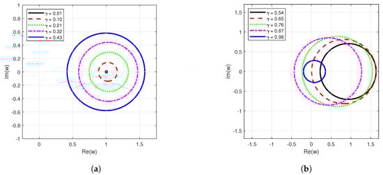
Figure 1. The boundaries of the closed disks in Table 1. The stability region of the linear discretization with two sub-domains for the indicated values of arbitrary non-integer order, (a) $\gamma =0.01,0.10,0.21,0.32,0.43$ and (b) $\gamma =0.54,0.65,0.76,0.87,0.98$, lies outside these circles.

In Figure 2, the stability regions for a quadratic approximation with $q=3$ and $q=5$ for $\gamma =0.21,0.54,0.98$ are presented. The stability region in the figure is the area outside the elliptical disks, which shows that the stability regions for $q=3$ and $q=5$ sub-domains are the same. However, in both cases, a varying number of eigenvalues with the potential to cross the stability threshold are obtained. For $q=3$, there is one non-zero dominant eigenvalue for $\gamma =0.21$ and $0.54$, and there are four non-zero eigenvalues for $\gamma =0.98$ with the potential to cross the stability threshold of 1. For $q=5$, $\gamma =0.21,0.54,0.98$ all have eight non-zero eigenvalues that can cross the stability threshold. However, when the intersection of the resulting stability regions from these eigenvalues is taken, the same stability region with $q=3$ is obtained for each illustrated $\gamma$ value, as shown in Figure 2. The figure shows that the numerical schemes for $\gamma =0.21$ and $\gamma =0.54$ are absolutely stable, and the scheme for $\gamma =0.98$ is not absolutely stable (conditional stability). Although a general conclusion about the stability of the numerical scheme cannot be made, it can be inferred from this analysis that whether the numerical scheme is absolutely or conditionally stable depends on the value of the arbitrary non-integer order of the fractional differential equation.

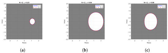
Figure 2. The stability regions of quadratic approximations with $q=3$ and $q=5$ for (a) $\gamma =0.21$, (b) $\gamma =0.54$ and (c) $\gamma =0.98$. The stability regions are the shaded areas located outside the elliptical disks.

4. Numerical Experimentation and Results

This section presents a series of numerical examples, ranging from single linear equations to systems of non-linear equations, along with the results. Detailed analyses of the results for each example are provided to illustrate key observations. For a comprehensive understanding of the numerical methods used in these examples, refer to the description provided in Section 3.

Example 1.

Consider the linear fractional differential equation [60]

$${ }_0^C{D}_t^{\gamma }u\left(t\right)+u\left(t\right)={\displaystyle \frac{2t^{2-\gamma }}{\Gamma (3-\gamma )}}-{\displaystyle \frac{t^{1-\gamma }}{\Gamma (2-\gamma )}}+t^2-t,0<\gamma \le 1,t\in [0,T],$$

(31)

with initial condition $u\left(0\right)=0$ and exact solution $u\left(t\right)=t^2-t$.

Table 2 presents the absolute error between the approximate and exact solutions using the non-overlapping multi-domain pseudospectral method with the CGL quadrature and the Chebyshev polynomials as the basis functions. The table also includes numerical results obtained without decomposing the domain. This comparative analysis highlights the accuracy and effectiveness of the multi-domain approach in reducing errors and improving the accuracy of the numerical solution. From the table, it can be seen that, for the fractional order of $\gamma =0.5$, although the maximum absolute error in the multi-domain setup does not decrease in terms of significant zeros, it reduces as q increases. This indicates that, although minimal, there is an advantage in using more sub-domains. Comparing the error to the single-domain result, there is an additional significant zero in the error of the multi-domain approach, which indicates that the multi-domain approach is more effective for this problem.

Table 2. Maximum absolute error for Example 1 in single-domain and multi-domain setups.

	$\mathit{N}=10,\mathit{\gamma }=0.5$			$\mathit{N}=10,\mathit{T}=6.0$
$\mathit{q}$	$\mathit{T}=\mathbf{1.0}$	$\mathit{T}=\mathbf{3.0}$	$\mathit{T}=\mathbf{6.0}$	$\mathit{\gamma }=\mathbf{0.2}$	$\mathit{\gamma }=\mathbf{0.6}$	$\mathit{\gamma }=\mathbf{0.8}$
5	$7.7426\times {10}^{-5}$	$6.2253\times {10}^{-4}$	$2.7903\times {10}^{-3}$	$1.3625\times {10}^{-3}$	$3.6161\times {10}^{-3}$	$5.2468\times {10}^{-3}$
10	$4.0800\times {10}^{-5}$	$5.2107\times {10}^{-4}$	$2.2192\times {10}^{-3}$	$6.7562\times {10}^{-4}$	$1.9440\times {10}^{-3}$	$2.8829\times {10}^{-3}$
20	$2.3538\times {10}^{-5}$	$4.4940\times {10}^{-4}$	$1.8850\times {10}^{-3}$	$4.4076\times {10}^{-4}$	$1.5245\times {10}^{-3}$	$2.1135\times {10}^{-3}$
50	$2.0489\times {10}^{-5}$	$4.1298\times {10}^{-4}$	$1.6596\times {10}^{-3}$	$3.8984\times {10}^{-4}$	$1.2966\times {10}^{-3}$	$1.5794\times {10}^{-3}$
100	$2.0286\times {10}^{-5}$	$4.0279\times {10}^{-4}$	$1.6132\times {10}^{-3}$	$3.8131\times {10}^{-4}$	$1.2746\times {10}^{-3}$	$1.4322\times {10}^{-3}$
200	$2.0374\times {10}^{-5}$	$4.0190\times {10}^{-4}$	$1.6047\times {10}^{-3}$	$3.8224\times {10}^{-4}$	$1.2946\times {10}^{-3}$	$1.3898\times {10}^{-3}$
	Single domain
	$3.3518\times {10}^{-4}$	$1.0362\times {10}^{-3}$	$2.1415\times {10}^{-3}$	$9.0794\times {10}^{-4}$	$2.5580\times {10}^{-3}$	$2.9839\times {10}^{-3}$

From Table 2, the effectiveness of the proposed numerical technique in obtaining an accurate approximate solution to a linear FDE is evident, so in the examples that follow, we consider non-linear FDEs to further validate the numerical method.

Example 2.

Consider the non-linear fractional differential equation [60]

$${ }_0^C{D}_t^{\gamma }u\left(t\right)-u^2\left(t\right)=-{\displaystyle \frac{2}{{(t+1)}^2}},0<\gamma \le 1,t\in [0,T],$$

(32)

where the initial condition is $u\left(0\right)=-2$ and the exact solution when $\gamma =1$ is given by $u\left(t\right)=-{\displaystyle \frac{2}{(t+1)}}$.

Table 3 shows the approximate solution obtained using two different sub-domains in the proposed method. The solutions in these sub-domains match the numerical values reported in Odibat and Momani [60]. It should be noted that closed-form solutions for $\gamma =0.2$ and $\gamma =0.4$ are not available. However, for $\gamma =1$, the accuracy of the proposed method is unquestionable. To further give credence to the accuracy of the proposed method, Table 4 demonstrates that the residual error is consistently close to zero for various values of $\gamma$. This suggests that the proposed method effectively resolves the problem in Example 2.

Table 3. Approximate solution of Example 2 using two different sub-domains, q, and the numerical values reported in Odibat and Momani [60].

t	$\mathit{\gamma }=0.2$			$\mathit{\gamma }=0.4$			$\mathit{\gamma }=1.0$
	$\mathit{q}=\mathbf{10}$	$\mathit{q}=\mathbf{20}$	Reported [60]	$\mathit{q}=\mathbf{10}$	$\mathit{q}=\mathbf{20}$	Reported [60]	$\mathit{q}=\mathbf{10}$	$\mathit{q}=\mathbf{20}$	Exact
0.0	−2.0000	−2.0000	−2.0000	−2.0000	−2.0000	−2.0000	−2.0000	−2.0000	−2.0000
0.2	−1.4454	−1.4455	−1.4864	−1.4874	−1.4874	−1.4899	−1.6666	−1.6666	−1.6666
0.4	−1.3295	−1.3296	−1.3665	−1.3506	−1.3506	−1.3525	−1.4285	−1.4285	−1.4285
0.6	−1.2477	−1.2478	−1.2822	−1.2525	−1.2526	−1.2541	−1.2500	−1.2500	−1.2500
0.8	−1.1867	−1.1868	−1.2192	−1.1774	−1.1774	−1.1787	−1.1111	−1.1111	−1.1111
1.0	−1.1396	−1.1397	−1.1704	−1.1177	−1.1178	−1.1189	−0.9999	−1.0000	−1.0000

Table 4. The residual errors of Example 2 at selected points using two different sub-domains, q, for different values of fractional order $\gamma$.

t	$\mathit{\gamma }=0.2$		$\mathit{\gamma }=0.4$		$\mathit{\gamma }=0.6$
	$\mathit{q}=\mathbf{10}$	$\mathit{q}=\mathbf{20}$	$\mathit{q}=\mathbf{10}$	$\mathit{q}=\mathbf{20}$	$\mathit{q}=\mathbf{10}$	$\mathit{q}=\mathbf{20}$
0.2	$4.4230\times {10}^{-9}$	$4.8561\times {10}^{-13}$	$9.7841\times {10}^{-11}$	$9.2539\times {10}^{-12}$	$3.2469\times {10}^{-10}$	$5.2865\times {10}^{-11}$
0.4	$9.3414\times {10}^{-13}$	$2.1760\times {10}^{-13}$	$1.6637\times {10}^{-11}$	$3.8897\times {10}^{-12}$	$9.3717\times {10}^{-11}$	$2.0417\times {10}^{-11}$
0.6	$4.9305\times {10}^{-13}$	$1.2423\times {10}^{-13}$	$8.9744\times {10}^{-12}$	$2.1446\times {10}^{-12}$	$4.9785\times {10}^{-11}$	$1.1396\times {10}^{-11}$
0.8	$2.8477\times {10}^{-13}$	$7.1831\times {10}^{-14}$	$5.4355\times {10}^{-12}$	$1.3228\times {10}^{-12}$	$3.0330\times {10}^{-11}$	$7.1187\times {10}^{-12}$
1.0	$1.7807\times {10}^{-13}$	$4.6629\times {10}^{-14}$	$3.5078\times {10}^{-12}$	$8.6397\times {10}^{-13}$	$1.9900\times {10}^{-11}$	$4.6949\times {10}^{-12}$

Example 3.

Next, consider the non-linear fractional differential equation [61]

$${ }_0^C{D}_t^{\gamma }u\left(t\right)+u{\left(t\right)}^2={\displaystyle \frac{2t^{2-\gamma }}{\Gamma (3-\gamma )}}-{\displaystyle \frac{t^{1-\gamma }}{\Gamma (2-\gamma )}}+{(t^2-t+1)}^2,0<\gamma \le 1,t\in [0,T],$$

(33)

with the initial condition $u\left(0\right)=1$ and whose exact solution is $u\left(t\right)=t^2-t+1$.

Table 5 presents the maximum absolute error of the difference between the exact and approximate solutions obtained using the multi-domain and single-domain methods. It is observed from the table that there is conformity with the trend observed in Table 2. As the domain of the FDE becomes larger, the error in the single domain scheme deteriorates; however, in comparison, the magnitude of the errors is better for the multi-domain scheme. We note that the magnitude of the error increases as $\gamma$ increases, similar to the trend observed in Table 2.

Table 5. The maximum absolute error of the difference between the exact and approximate solutions of Example 3 for different numbers of sub-domains, q.

	$\mathit{N}=10,\mathit{\gamma }=0.5$			$\mathit{N}=10,\mathit{T}=6.0$
$\mathit{q}$	$\mathit{T}=\mathbf{1.0}$	$\mathit{T}=\mathbf{3.0}$	$\mathbf{T}=\mathbf{6.0}$	$\mathit{\gamma }=\mathbf{0.2}$	$\mathit{\gamma }=\mathbf{0.6}$	$\mathit{\gamma }=\mathbf{0.8}$
5	$6.5833\times {10}^{-5}$	$4.5300\times {10}^{-4}$	$7.7010\times {10}^{-4}$	$1.6897\times {10}^{-4}$	$9.9126\times {10}^{-4}$	$1.0256\times {10}^{-3}$
10	$3.6216\times {10}^{-5}$	$2.6020\times {10}^{-4}$	$4.7125\times {10}^{-4}$	$1.0248\times {10}^{-4}$	$6.3577\times {10}^{-4}$	$7.4647\times {10}^{-4}$
20	$1.9347\times {10}^{-5}$	$1.3492\times {10}^{-4}$	$2.8073\times {10}^{-4}$	$5.5876\times {10}^{-5}$	$3.9608\times {10}^{-4}$	$5.1975\times {10}^{-4}$
50	$1.6865\times {10}^{-5}$	$8.2634\times {10}^{-5}$	$1.3621\times {10}^{-4}$	$2.3143\times {10}^{-5}$	$2.0636\times {10}^{-4}$	$3.2248\times {10}^{-4}$
100	$1.6547\times {10}^{-5}$	$6.7163\times {10}^{-5}$	$8.2558\times {10}^{-5}$	$1.0361\times {10}^{-5}$	$1.1932\times {10}^{-4}$	$2.1211\times {10}^{-4}$
200	$1.6576\times {10}^{-5}$	$5.9548\times {10}^{-5}$	$6.7326\times {10}^{-5}$	$7.5375\times {10}^{-6}$	$7.6523\times {10}^{-5}$	$1.3480\times {10}^{-4}$
	Single domain
	$3.1847\times {10}^{-4}$	$9.0415\times {10}^{-4}$	$1.7639\times {10}^{-3}$	$6.1773\times {10}^{-4}$	$1.9684\times {10}^{-3}$	$2.2669\times {10}^{-3}$

Example 4.

Consider the initial value fractional homogeneous Bagley–Torvik differential equation

$${ }_0^C{D}_t^{\gamma }u\left(t\right)+u^{″}\left(t\right)+u\left(t\right)=0,fort\in (0,T]and\gamma \in (1,2),$$

(34)

subject to the initial conditions $u\left(0\right)=1.0$ and $u^{\prime }\left(0\right)=0$.

If we replace the right-hand side of Equation (34) with $2+4\sqrt{{\displaystyle \frac{t}{\pi }}}+t^2$ and set $t\in (0,1]$, subject to the starting conditions $u\left(0\right)=0.0$ and $u^{\prime }\left(0\right)=0$, the closed-form solution is given as $u\left(t\right)=t^2$ when $\gamma =1.5$. Table 6 presents the errors obtained by taking the absolute value of the difference between the numerical solutions obtained through the multi-domain technique and the exact solutions, and these are compared with the errors obtained through the evolutionary artificial neural networks method in the study of Raja et al. [62].

Table 6. The absolute errors of the difference between the exact and numerical solutions of Example 4 at different t values using $N=12$ and $q=400$ in comparison with the errors reported in the work of Raja et al. [62].

t	Exact Solution	Present Result	Present Error	Reported Error [62]
0.1	$0.01$	$0.01000$	$1.83183\times {10}^{-7}$	$5.48\times {10}^{-5}$
0.3	$0.09$	$0.09005$	$1.26966\times {10}^{-6}$	$2.66\times {10}^{-3}$
0.5	$0.25$	$0.25014$	$6.69388\times {10}^{-6}$	$1.67\times {10}^{-2}$
0.7	$0.49$	$0.49026$	$3.40281\times {10}^{-5}$	$5.80\times {10}^{-2}$
0.9	$0.81$	$0.81040$	$1.25968\times {10}^{-4}$	$1.50\times {10}^{-1}$
1.0	$1.00$	$1.00048$	$2.12565\times {10}^{-4}$	$2.25\times {10}^{-1}$

Table 6 compares the exact and approximate solutions obtained using the multi-domain method at various t values and the associated errors at each t. The errors are compared with those obtained in Raja et al. [62]. It is observed from the table that the approximate solutions match the exact solutions better than the results in Raja et al. [62], and this validates the efficiency of the proposed method as it outperforms a neural network approach known to be efficient and reliable.

To further validate the accuracy of the proposed multi-domain method, the infinity norm of the residual for different numbers of sub-domains is presented. Table 7 gives the infinity norm of the residual errors for Example 4. The residual error is obtained through the discrete equivalent of Equation (34), defined by

$$\begin{array}{cc}\hfill \mathrm{Residual}=& \sum _{e=1}^l{\left({ }_{t_{e-1},t_e}{\mathbf{D}}_e^{\gamma }\right)}^{\mathsf{T}}{\mathbf{U}}_{h_l,e}+{\left({ }_{t_l,h_l}{\mathbf{D}}_l^{\gamma }\right)}^{\mathsf{T}}{\mathbf{U}}_{h_l,l}+{\left({ }_{t_l,h_l}{\mathbf{D}}_l^2\right)}^{\mathsf{T}}{\mathbf{U}}_{h_l,l}+{\mathbf{E}}_l^{\mathsf{T}}{\mathbf{U}}_{h_l,l}.\hfill \end{array}$$

(35)

Table 7. The maximum residual errors for Example 4 for different T values, fractional orders, and different numbers of multi-domains, q.

	$\mathit{N}=10,\mathit{\gamma }=1.5$			$\mathit{N}=10,\mathit{T}=6.0$
$\mathit{q}$	$\mathit{T}=\mathbf{1}.\mathbf{0}$	$\mathit{T}=\mathbf{3}.\mathbf{0}$	$\mathit{T}=\mathbf{6}.\mathbf{0}$	$\mathit{\gamma }=\mathbf{1}.\mathbf{2}$	$\mathit{\gamma }=\mathbf{1}.\mathbf{6}$	$\mathit{\gamma }=\mathbf{1}.\mathbf{8}$
10	$1.115\times {10}^{-10}$	$1.158\times {10}^{-11}$	$1.933\times {10}^{-12}$	$1.031\times {10}^{-12}$	$1.870\times {10}^{-12}$	$3.445\times {10}^{-12}$
20	$7.346\times {10}^{-10}$	$6.618\times {10}^{-11}$	$1.158\times {10}^{-11}$	$1.078\times {10}^{-11}$	$2.104\times {10}^{-11}$	$2.765\times {10}^{-11}$

Table 7 shows that the method is efficient in solving fractional-order differential equations of varying values of arbitrary non-integer order, as the residual error remains very small for various fractional orders, demonstrating the effectiveness of the multi-domain technique.

To further validate the results obtained, we reproduce the solution profiles obtained by Zafar et al. [63] and observe excellent agreement in the result, as shown in Figure 3.

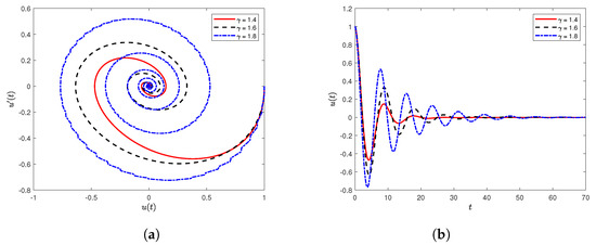
Figure 3. The dynamics of the Bagley–Torvik Equation (34) for various values of $\gamma$ with $T=70$, $N=10$ and $q=400$: (a) the phase portrait for the $u-u^{\prime }$ plane and (b) the $u\left(t\right)$ profile.

In the remaining examples in this section, we consider systems of coupled fractional initial value problems that describe chaotic systems. These equations often exhibit long-term dynamics and, invariably, require long-term integration to fully understand the underlying dynamics involved. Therefore, a numerical technique, such as the multi-domain Chebyshev pseudospectral method, that can handle long-term integration is a perfect fit for solving such systems, as corroborated by the results in the next four examples.

Example 5.

Consider the fractional chaotic system of differential equations which describe a memory-inherent electrical system [64]

$$\left.\begin{array}{cc}\hfill & { }_0^C{D}_t^{\gamma }{u}_1\left(t\right)={\displaystyle \frac{u_2\left(t\right)}{c}},\hfill \\ \hfill & { }_0^C{D}_t^{\gamma }{u}_2\left(t\right)=-{\displaystyle \frac{1}{L}}\left(u_1\left(t\right)+\beta u_2\left(t\right){\left(u_3\left(t\right)\right)}^2-\beta u_2\left(t\right)\right),\hfill \\ \hfill & { }_0^C{D}_t^{\gamma }{u}_3\left(t\right)=-u_2\left(t\right)-\alpha u_3\left(t\right)+u_2\left(t\right)u_3\left(t\right),t\in (0,T],\gamma \in (0,1],\hfill \end{array}\right\}$$

(36)

subject to the following initial state, $(0.1,0.0,0.1)$. Here, $c=0.70,L=3.00,\beta =1.10$ and $\alpha =0.60$. The voltage across the capacitor, c, is represented by the variable $u_1\left(t\right)$, and the current through the inductor, L, is represented by the variable $u_2\left(t\right)$, and the internal state of the memristive system is denoted by the variable $u_3\left(t\right)$.

The average maximum residual error for the system (36) is given in Table 8. We remark here that the maximum residual errors presented in Table 8 and subsequent tables in this section are obtained as the average of the maximum residuals of the equations in the system. The residuals are calculated similarly to Equation (35). It can be seen from Table 8 that for various fractional orders and seemingly large domains, $[0,T]$, a high level of accuracy is obtained when the multi-domain Chebyshev pseudospectral method is used. Due to the inherently chaotic nature of the problem, the dynamics of the system typically require a large physical domain to fully develop, and to effectively capture these complex long-term behaviors, the physical domain is partitioned into a large number of smaller sub-domains. The table shows that the average of the maximum residual errors decreases marginally as the number of sub-domains increases. This inverse relationship between the number of sub-domains and the residual error highlights the applicability of the multi-domain technique when dealing with this kind of system that requires long-term integration. This is particularly evident when the error is compared to the error associated with the single-domain method. As already observed in the previous examples and now corroborated by Table 8, the error associated with the single-domain method is worse than the error obtained when the multi-domain approach is used.

Table 8. The residual errors for Example 5 for two values of T using $N=10$ and for different numbers of sub-domains q, with $c=0.70,L=3.00,\beta =1.10$ and $\alpha =0.60$.

	$\mathit{T}=20.0$			$\mathit{T}=50.0$
$\mathit{q}$	$\mathit{\gamma }=\mathbf{0}.\mathbf{7}$	$\mathit{\gamma }=\mathbf{0}.\mathbf{8}$	$\mathit{\gamma }=\mathbf{0}.\mathbf{9}$	$\mathit{\gamma }=\mathbf{0}.\mathbf{7}$	$\mathit{\gamma }=\mathbf{0}.\mathbf{8}$	$\mathit{\gamma }=\mathbf{0}.\mathbf{9}$
100	$2.515\times {10}^{-11}$	$7.810\times {10}^{-12}$	$8.503\times {10}^{-12}$	$8.781\times {10}^{-11}$	$3.336\times {10}^{-11}$	$8.054\times {10}^{-10}$
200	$9.780\times {10}^{-12}$	$2.590\times {10}^{-12}$	$2.144\times {10}^{-12}$	$3.434\times {10}^{-11}$	$1.113\times {10}^{-11}$	$1.935\times {10}^{-10}$
300	$5.544\times {10}^{-12}$	$1.365\times {10}^{-12}$	$9.795\times {10}^{-13}$	$1.973\times {10}^{-11}$	$5.817\times {10}^{-12}$	$8.468\times {10}^{-11}$
400	$3.717\times {10}^{-12}$	$8.632\times {10}^{-13}$	$5.718\times {10}^{-13}$	$1.319\times {10}^{-11}$	$3.701\times {10}^{-12}$	$4.723\times {10}^{-11}$
500	$2.720\times {10}^{-12}$	$6.125\times {10}^{-13}$	$4.095\times {10}^{-13}$	$9.769\times {10}^{-12}$	$2.592\times {10}^{-12}$	$3.004\times {10}^{-11}$
	Single domain
	$2.397\times {10}^{-9}$	$2.439\times {10}^{-9}$	$1.920\times {10}^{-7}$	$3.101\times {10}^{-8}$	$4.108\times {10}^{-7}$	$5.427\times {10}^{-7}$

To lend further credibility to the numerical results of this example, we reproduce the dynamics, in the form of phase portraits, of the memristive chaotic electrical system as reported in the work of Sene [64]. As shown in Figure 4, there is an excellent agreement between these phase portraits and those in the work of Sene [64].

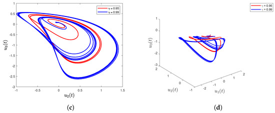
Figure 4. The phase portraits of the chaotic systems (36) for the (a) $u_1-u_2$ plane, (b) $u_1-u_3$ plane, (c) $u_2-u_3$ plane and (d) $u_1-u_2-u_3$ surface with $\gamma =0.95$ and $0.99$, $T=250,N=13$ and $q=850$.

Example 6.

Consider the fractional modified stretch-twist-fold differential equations [65]

$$\left.\begin{array}{cc}\hfill & { }_0^C{D}_t^{\gamma }{u}_1\left(t\right)={\Omega }_1{u}_3\left(t\right)-8u_1\left(t\right)u_2\left(t\right),t\in (0,T],\gamma \in (0,1],\hfill \\ \hfill & { }_0^C{D}_t^{\gamma }{u}_2\left(t\right)=11{\left(u_1\left(t\right)\right)}^2+3{\left(u_2\left(t\right)\right)}^2+{\left(u_3\left(t\right)\right)}^2+{\Omega }_2{u}_1\left(t\right)u_3\left(t\right)-3{\Omega }_3^2,\hfill \\ \hfill & { }_0^C{D}_t^{\gamma }{u}_3\left(t\right)=2\left(1-{\Omega }_4\right)u_2\left(t\right)u_3\left(t\right)-{\Omega }_1{u}_1\left(t\right)-{\Omega }_2{u}_1\left(t\right)u_2\left(t\right),\hfill \end{array}\right\}$$

(37)

under the initial state $(0.2,-0.2,0.2)$, with $\gamma =1.00,{\Omega }_1=0.2,{\Omega }_2=2.0,{\Omega }_3=1.0$ and ${\Omega }_4=0.1$.

Similar to the previous example, this system typically requires a large physical domain to fully stabilize and develop, and when solved on a single domain, the numerical solution is unstable, as evidenced by the average residual errors in a single domain presented in Table 9. We present the average maximum residual errors for various fractional orders and relatively large domains, $[0,T]$, for different relatively large numbers of sub-domains in Table 9. There is an agreement between the level of accuracy observed for the results in Table 9 and those obtained in the previous examples. The error obtained for the various sub-domain numbers used is shown to be small, indicating that the proposed multi-domain Chebyshev pseudospectral method efficiently solves this system of FDEs. As q increases, it is observed that the average residual error improves, resulting in higher accuracy. The superior effectiveness of the multi-domain approach over the single-domain numerical scheme becomes marginally clearer in this example. In this case, the single-domain numerical scheme is observed to produce quite large numerical errors, whereas the multi-domain technique can achieve a higher accuracy level. This disparity in the level of performance highlights the limitation in the scope of the single-domain scheme, while the multi-domain approach demonstrates robustness and versatility, especially for complex systems like the one considered in this example.

Table 9. The average maximum residual errors for Example 6 for two values of T and different numbers of sub-domains q using $N=10$. The following parameter values are used: ${\Omega }_1=0.2$, ${\Omega }_2=2.0,{\Omega }_3=1.0$ and ${\Omega }_4=0.1$.

	$\mathit{T}=20.0$			$\mathit{T}=50.0$
$\mathit{q}$	$\mathit{\gamma }=\mathbf{0}.\mathbf{7}$	$\mathit{\gamma }=\mathbf{0}.\mathbf{8}$	$\mathit{\gamma }=\mathbf{0}.\mathbf{9}$	$\mathit{\gamma }=\mathbf{0}.\mathbf{7}$	$\mathit{\gamma }=\mathbf{0}.\mathbf{8}$	$\mathit{\gamma }=\mathbf{0}.\mathbf{9}$
100	$1.292\times {10}^{-8}$	$4.793\times {10}^{-8}$	$2.171\times {10}^{-8}$	$1.364\times {10}^{-10}$	$1.059\times {10}^{-8}$	$4.952\times {10}^{-8}$
200	$1.883\times {10}^{-8}$	$1.192\times {10}^{-8}$	$6.393\times {10}^{-9}$	$1.060\times {10}^{-8}$	$2.928\times {10}^{-8}$	$4.607\times {10}^{-8}$
300	$8.108\times {10}^{-9}$	$5.539\times {10}^{-9}$	$3.267\times {10}^{-9}$	$1.826\times {10}^{-8}$	$3.502\times {10}^{-8}$	$1.144\times {10}^{-8}$
400	$4.546\times {10}^{-9}$	$3.223\times {10}^{-9}$	$1.790\times {10}^{-9}$	$2.750\times {10}^{-8}$	$1.284\times {10}^{-8}$	$1.065\times {10}^{-8}$
500	$3.082\times {10}^{-9}$	$2.098\times {10}^{-9}$	$1.182\times {10}^{-9}$	$1.883\times {10}^{-8}$	$1.194\times {10}^{-8}$	$6.393\times {10}^{-9}$
	Single domain
	$1.730\times {10}^1$	$1.999\times {10}^1$	$2.419\times {10}^1$	$8.388\times {10}^1$	$2.195\times {10}^{-1}$	$4.131\times {10}^1$

Figure 5 gives the behavior of the solution profiles as t evolves. The results are as expected and in complete agreement with the result of Azam et al. [65]. It is also observed in Figure 6 that the chaotic system flows through the various states by turning and twisting about the quadrants. This dynamics was also captured by Azam et al. [65] and validates the numerical results being put forward in this study.

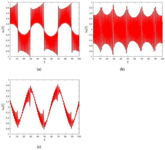
Figure 5. The time evolution of $u_1\left(t\right)$, $u_2\left(t\right)$, $u_3\left(t\right)$ of the chaotic system (37) with $\gamma =1.00,$${\Omega }_1=0.2,$$T=100,N=13$ and $q=350$.

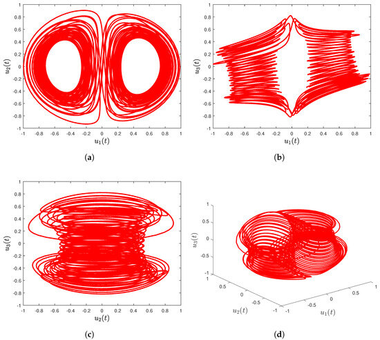
Figure 6. The phase portraits of the chaotic system (37) for the (a) $u_1-u_2$ plane, (b) $u_1-u_3$ plane, (c) $u_2-u_3$ plane and (d) $u_1-u_2-u_3$ surface with $\gamma =1.00,{\Omega }_1=0.2,T=100,N=13$ and $q=350$.

Example 7.

Consider the fractional Rossler differential equations [66]

$$\left.\begin{array}{cc}\hfill & { }_0^C{D}_t^{\gamma }{u}_1\left(t\right)=-u_2\left(t\right)-u_3\left(t\right),t\in (0,T],\gamma \in (0,1],\hfill \\ \hfill & { }_0^C{D}_t^{\gamma }{u}_2\left(t\right)=u_1\left(t\right)+{\Psi }_1{u}_2\left(t\right),\hfill \\ \hfill & { }_0^C{D}_t^{\gamma }{u}_3\left(t\right)=0.2+u_1\left(t\right)u_3\left(t\right)-10u_3\left(t\right),\hfill \end{array}\right\}$$

(38)

with the following initial conditions: $(1,1,1)$, with ${\Psi }_1=0.4$ and $\gamma =0.9$.

Table 10 shows the average maximum residual errors for Equation (38) for selected values of arbitrary non-integer order, $\gamma$, and for two domains, $(0,T]$. The results are presented for different numbers of domain decomposition. From Table 10, we see that the residual errors are small, indicating that the approximate solutions are accurate. As has been validated several times in this study, an increase in the number of sub-domains used results in more accurate solutions. It is also shown that using the single-domain approach results in less accuracy in the approximate solutions obtained.

Table 10. The residual errors for Example 7 at two final times T using the number of grid points $N=10$ for different numbers of sub-domains q and ${\Psi }_1=0.40$.

	$\mathit{T}=20.0$			$\mathit{T}=50.0$
$\mathit{q}$	$\mathit{\gamma }=\mathbf{0}.\mathbf{7}$	$\mathit{\gamma }=\mathbf{0}.\mathbf{8}$	$\mathit{\gamma }=\mathbf{0}.\mathbf{9}$	$\mathit{\gamma }=\mathbf{0}.\mathbf{7}$	$\mathit{\gamma }=\mathbf{0}.\mathbf{8}$	$\mathit{\gamma }=\mathbf{0}.\mathbf{9}$
100	$1.073\times {10}^{-7}$	$4.973\times {10}^{-8}$	$1.171\times {10}^{-8}$	$1.469\times {10}^{-7}$	$1.469\times {10}^{-7}$	$1.893\times {10}^{-7}$
200	$5.544\times {10}^{-8}$	$1.857\times {10}^{-8}$	$3.569\times {10}^{-9}$	$1.269\times {10}^{-7}$	$6.666\times {10}^{-8}$	$4.696\times {10}^{-8}$
300	$3.479\times {10}^{-8}$	$1.015\times {10}^{-8}$	$1.740\times {10}^{-9}$	$9.241\times {10}^{-8}$	$3.853\times {10}^{-8}$	$3.299\times {10}^{-8}$
400	$2.459\times {10}^{-8}$	$6.520\times {10}^{-9}$	$1.042\times {10}^{-9}$	$6.979\times {10}^{-8}$	$2.574\times {10}^{-8}$	$1.933\times {10}^{-8}$
500	$1.859\times {10}^{-8}$	$4.653\times {10}^{-9}$	$7.023\times {10}^{-10}$	$5.544\times {10}^{-8}$	$1.857\times {10}^{-8}$	$1.189\times {10}^{-8}$
	Single domain
	$1.594\times {10}^{-4}$	$2.218\times {10}^{-4}$	$6.733\times {10}^{-5}$	$1.725\times {10}^{-4}$	$2.518\times {10}^{-4}$	$3.726\times {10}^{-4}$

Figure 7 displays the phase portraits for the chaotic system, and the result agrees with the results obtained in Li et al. [66], thereby validating the present numerical solutions.

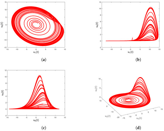
Figure 7. The phase portraits of the chaotic systems (38) for the (a) $u_1$-$u_2$ plane, (b) $u_1-u_3$ plane, (c) $u_2-u_3$ plane and (d) $u_1-u_2-u_3$ surface with $\gamma =0.90,{\Psi }_1=0.4,T=200,N=10$ and $q=900$.

Example 8.

Consider the following non-linear fractional chaotic system [67]

$$\left.\begin{array}{cc}\hfill & { }_0^C{D}_t^{\gamma }{u}_1\left(t\right)={\Psi }_1{u}_1\left(t\right)+u_2\left(t\right)+u_2\left(t\right)u_3\left(t\right),t\in (0,T],\gamma \in (0,1],\hfill \\ \hfill & { }_0^C{D}_t^{\gamma }{u}_2\left(t\right)=-u_1\left(t\right)u_3\left(t\right)+u_2\left(t\right)u_3\left(t\right),\hfill \\ \hfill & { }_0^C{D}_t^{\gamma }{u}_3\left(t\right)=-{\Psi }_2{u}_3\left(t\right)-{\Psi }_3{u}_1\left(t\right)u_2\left(t\right)-m_1,\hfill \end{array}\right\}$$

(39)

with the initial state given as $(0.2,0.2,0.2)$, ${\Psi }_1={\Psi }_2={\Psi }_3=1.0,m_1=0.0$ and $\gamma =0.9$.

In Table 11, the average maximum residual errors obtained for Equation (39) are presented. The table shows that an increase in the number of partitioned domains results in higher accuracy of approximate solutions obtained for the selected fractional orders and domains. The average maximum residual errors are observed to be small, confirming that the proposed multi-domain method is highly efficient for this fractional differential model, unlike the single-domain approach, which is not as accurate.

Table 11. The average maximum residual errors for Example 8 in two different domains $(0,T]$ with $N=10$ for different numbers of sub-domains q, ${\Psi }_1={\Psi }_2={\Psi }_3=1.0$ and $m_1=0.0$.

	$\mathit{T}=20.0$			$\mathit{T}=50.0$
$\mathit{q}$	$\mathit{\gamma }=\mathbf{0}.\mathbf{7}$	$\mathit{\gamma }=\mathbf{0}.\mathbf{8}$	$\mathit{\gamma }=\mathbf{0}.\mathbf{9}$	$\mathit{\gamma }=\mathbf{0}.\mathbf{7}$	$\mathit{\gamma }=\mathbf{0}.\mathbf{8}$	$\mathit{\gamma }=\mathbf{0}.\mathbf{9}$
100	$4.114\times {10}^{-8}$	$6.012\times {10}^{-8}$	$5.802\times {10}^{-8}$	$2.142\times {10}^{-7}$	$1.226\times {10}^{-7}$	$2.711\times {10}^{-7}$
200	$1.305\times {10}^{-8}$	$1.673\times {10}^{-8}$	$1.559\times {10}^{-8}$	$5.335\times {10}^{-8}$	$6.845\times {10}^{-8}$	$7.236\times {10}^{-8}$
300	$6.155\times {10}^{-9}$	$7.361\times {10}^{-9}$	$7.034\times {10}^{-9}$	$3.422\times {10}^{-8}$	$4.357\times {10}^{-8}$	$4.049\times {10}^{-8}$
400	$3.398\times {10}^{-9}$	$4.196\times {10}^{-9}$	$3.935\times {10}^{-9}$	$2.050\times {10}^{-8}$	$2.575\times {10}^{-8}$	$2.436\times {10}^{-8}$
500	$2.195\times {10}^{-9}$	$2.720\times {10}^{-9}$	$2.540\times {10}^{-9}$	$1.304\times {10}^{-8}$	$1.676\times {10}^{-8}$	$1.559\times {10}^{-8}$
	Single domain
	$3.055\times {10}^{-2}$	$1.225\times {10}^{-2}$	$9.667\times {10}^{-1}$	$2.279\times {10}^{-2}$	$6.453\times {10}^1$	$4.708\times {10}^1$

We present the phase portraits of the chaotic system in Figure 8. The figure validates the dynamics reported by Sene [67] and is in excellent agreement with the previously published result. The agreement between the phase portraits presented here and those documented in the study by Sene [67] serves to further corroborate the accuracy and reliability of the current numerical method.

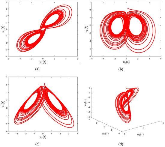
Figure 8. The phase portraits of the chaotic systems (39) for the (a) $u_1-u_2$ plane, (b) $u_1-u_3$ plane, (c) $u_2-u_3$ plane and (d) $u_1-u_2-u_3$ surface with $\gamma =0.95,T=150,N=10$ and $q=800$.

Figure 9 shows the phase portraits of the chaotic system in Equation (39) using two different $\gamma$ values. The figure justifies that the dynamics of the chaotic system depend on the arbitrary real order.

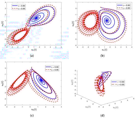
Figure 9. The phase portraits of the chaotic systems (39) for the (a) $u_1-u_2$ plane, (b) $u_1-u_3$ plane, (c) $u_2-u_3$ plane and (d) $u_1-u_2-u_3$ surface with $\gamma =0.90and0.95,T=80,N=10$ and $q=350$.

Figure 10 displays the accuracy of the numerical results (the maximum absolute residual in each sub-domain) of each equation in the chaotic systems presented in Equations (36)–(39). The figures show that the accuracy of the solutions obtained through the multi-domain Chebyshev pseudospectral method is high and sometimes reaches errors smaller than those reported so far in the tables. As can be clearly observed, as the number of sub-domains in the computational domain increases, the residual error decreases correspondingly. In some instances, the residual error is reduced to the order of ${10}^{-16}$. However, the residual errors with a small number of sub-domains already show good accuracy, thereby showing that using the multi-domain approach proposed in this study is very efficient in solving fractional differential equations that typically require long-term integration.

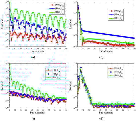
Figure 10. The maximum residual error in each domain for (a) Equation (36) (b) Equation (37) (c) Equation (38) and (d) Equation (39) using $\gamma =0.8,T=50,N=10$ and $q=100$.

5. Conclusions

This study introduced a novel approach, the multi-domain Chebyshev pseudospectral method for solving fractional differential equations. The novelty of the method stemmed from the use of non-overlapping multi-domains, Chebyshev polynomials of the first kind and Gauss–Lobatto collocation points in developing the scheme, which was specifically adapted to handle fractional differential equations. The method leverages the global properties of spectral-based methods for discretizing non-local operators such as fractional differential operators, the exponential convergence of the Chebyshev polynomial-based pseudospectral method and the multi-domain approach’s ability to maintain the accuracy of solutions to problems with long-term dynamics. The stability region of the multi-domain scheme was established through linear stability analysis. The stability analysis showed that obtaining an absolute and Lubich-stable numerical scheme for some values of arbitrary non-integer order is possible. Several numerical experiments involving linear and non-linear single FDEs and systems of non-linear FDEs were conducted. The examples were carefully chosen to span varying complexity levels, including fractional initial value problems with long-term dynamics, such as chaotic systems, which were shown to significantly benefit from a multi-domain numerical scheme. These examples have established that the proposed multi-domain numerical method gives highly accurate results. To validate the method, comparisons of the numerical results obtained in this study were made with analytical solutions, where available, and approximate solutions from the literature. It was found that the proposed method gave more accurate solutions than the approximate solutions from the literature. Where an exact solution was unavailable, residual error analysis was conducted to establish the accuracy of the proposed method. In all the examples considered, the method was found to produce comparative, highly accurate solutions. In future studies, we will explore the applicability of the Chebyshev pseudospectral method in non-overlapping or overlapping partitioned domains to fractional boundary value problems with non-linear dynamics.

References

- Podlubny, I. Fractional Differential Equations: An Introduction to Fractional Derivatives, Fractional Differential Equations, to Methods of Their Solution and Some of Their Applications; Elsevier: Amsterdam, The Netherlands, 1998. [Google Scholar]
- Oldham, K.; Spanier, J. The Fractional Calculus Theory and Applications of Differentiation and Integration to Arbitrary Order; Elsevier: Amsterdam, The Netherlands, 1974. [Google Scholar]
- Caputo, M.; Fabrizio, M. A new definition of fractional derivative without singular kernel. Prog. Fract. Differ. Appl. 2015, 1, 73–85. [Google Scholar]
- Atangana, A.; Baleanu, D. New fractional derivatives with nonlocal and non-singular kernel: Theory and application to heat transfer model. arXiv 2016, arXiv:1602.03408. [Google Scholar] [CrossRef]
- Javadi, R.; Mesgarani, H.; Nikan, O.; Avazzadeh, Z. Solving fractional order differential equations by using fractional radial basis function neural network. Symmetry 2023, 15, 1275. [Google Scholar] [CrossRef]
- Benchochra, M.; Karapinar, E.; Lazreg, J.E.; Salim, A. Fractional Differential Equations: New Advancements for Generalized Fractional Derivatives; Springer: Cham, Switzerland, 2023. [Google Scholar]
- Ahmadian, S.; Darvishi, M. Fractional version of (1+1)-dimensional Biswas–Milovic equation and its solutions. Optik 2016, 127, 10135–10147. [Google Scholar] [CrossRef]
- Manafian, J.; Lakestani, M. A new analytical approach to solve some of the fractional-order partial differential equations. Indian J. Phys. 2017, 91, 243–258. [Google Scholar] [CrossRef]
- Kumar, S.; Kumar, D.; Abbasbandy, S.; Rashidi, M. Analytical solution of fractional Navier–Stokes equation by using modified Laplace decomposition method. Ain Shams Eng. J. 2014, 5, 569–574. [Google Scholar] [CrossRef]
- Shakeel, M.; Mohyud-Din, S.T. A novel (G′/G)-expansion method and its application to the space-time fractional symmetric regularized long wave (SRLW) equation. Adv. Trends Math. 2015, 2, 1–16. [Google Scholar] [CrossRef]
- Zhu, Q.; Qi, J. Exact Solutions of the Nonlinear Space-Time Fractional Partial Differential Symmetric Regularized Long Wave (SRLW) Equation by Employing Two Methods. Adv. Math. Phys. 2022, 2022, 8062119. [Google Scholar] [CrossRef]
- Senol, M. New analytical solutions of fractional symmetric regularized-long-wave equation. Rev. Mex. De Física 2020, 66, 297–307. [Google Scholar] [CrossRef]
- Ünal, S.Ç.; Daşcıoğlu, A.; Bayram, D.V. Jacobi elliptic function solutions of space-time fractional symmetric regularized long wave equation. Math. Sci. Appl. E-Notes 2021, 9, 53–63. [Google Scholar] [CrossRef]
- Tuluce Demiray, S.; Bulut, H.; Belgacem, F.B.M. Sumudu transform method for analytical solutions of fractional type ordinary differential equations. Math. Probl. Eng. 2015, 2015, 131690. [Google Scholar] [CrossRef]
- Kumar, D.; Darvishi, M.; Joardar, A. Modified Kudryashov method and its application to the fractional version of the variety of Boussinesq-like equations in shallow water. Opt. Quantum Electron. 2018, 50, 128. [Google Scholar] [CrossRef]
- He, J.H. Exp-function method for fractional differential equations. Int. J. Nonlinear Sci. Numer. Simul. 2013, 14, 363–366. [Google Scholar] [CrossRef]
- Ahmadian, S.; Darvishi, M. A new fractional Biswas–Milovic model with its periodic soliton solutions. Optik 2016, 127, 7694–7703. [Google Scholar] [CrossRef]
- Turan, D.A. A sine-cosine wavelet method for the approximation solutions of the fractional Bagley-Torvik equation. Sigma J. Eng. Nat. Sci. Ve Fen Bilim. Derg. 2022, 40, 150–154. [Google Scholar]
- Khan, A.; Shah, K.; Luo, D. Numerical Solutions to Some Families of Fractional Order Differential Equations by Laguerre Polynomials. In Nonlinear Systems-Theoretical Aspects and Recent Applications; IntechOpen: London, UK, 2020. [Google Scholar]
- Sun, Z.Z.; Gao, G.H. Fractional Differential Equations: Finite Difference Methods; Walter de Gruyter GmbH & Co KG: Berlin, Germany, 2020. [Google Scholar]
- Hattaf, K.; Hajhouji, Z.; Ait Ichou, M.; Yousfi, N. A numerical method for fractional differential equations with new generalized Hattaf fractional derivative. Math. Probl. Eng. 2022, 2022, 3358071. [Google Scholar] [CrossRef]
- Kumar, M.; Jhinga, A.; Daftardar-Gejji, V. Higher order numerical methods for fractional delay differential equations. Indian J. Pure Appl. Math. 2024, 1–22. [Google Scholar] [CrossRef]
- Jhinga, A.; Daftardar-Gejji, V. A new numerical method for solving fractional delay differential equations. Comput. Appl. Math. 2019, 38, 166. [Google Scholar] [CrossRef]
- Lee, S.; Kim, H.; Jang, B. A Novel Numerical Method for Solving Nonlinear Fractional-Order Differential Equations and Its Applications. Fractal Fract. 2024, 8, 65. [Google Scholar] [CrossRef]
- Kumar, S.; Shaw, P.K.; Abdel-Aty, A.H.; Mahmoud, E.E. A numerical study on fractional differential equation with population growth model. Numer. Methods Partial Differ. Equations 2024, 40, e22684. [Google Scholar] [CrossRef]
- Bhrawy, A.H.; Taha, T.M.; Machado, J.A.T. A review of operational matrices and spectral techniques for fractional calculus. Nonlinear Dyn. 2015, 81, 1023–1052. [Google Scholar] [CrossRef]
- Baleanu, D.; Bhrawy, A.; Taha, T. A modified generalized Laguerre spectral method for fractional differential equations on the half line. In Proceedings of the Abstract and Applied Analysis; Wiley Online Library: Hoboken, NJ, USA, 2013; Volume 2013, p. 413529. [Google Scholar]
- Delkhosh, M.; Parand, K. A new computational method based on fractional Lagrange functions to solve multi-term fractional differential equations. Numer. Algorithms 2021, 88, 729–766. [Google Scholar] [CrossRef]
- Xu, Q.; Zheng, Z. Spectral collocation method for fractional differential/integral equations with generalized fractional operator. Int. J. Differ. Equations 2019, 2019, 3734617. [Google Scholar] [CrossRef]
- Raslan, K.R.; Abd El Salam, M.A.; Ali, K.K.; Mohamed, E.M. Spectral Tau method for solving general fractional order differential equations with linear functional argument. J. Egypt. Math. Soc. 2019, 27, 33. [Google Scholar] [CrossRef]
- Shen, J.; Sheng, C. Spectral methods for fractional differential equations using generalized Jacobi functions. Handb. Fract. Calc. Appl. Numer. Methods 2019, 3, 127–155. [Google Scholar]
- Zayernouri, M.; Karniadakis, G.E. Exponentially accurate spectral and spectral element methods for fractional ODEs. J. Comput. Phys. 2014, 257, 460–480. [Google Scholar] [CrossRef]
- Zhao, J.; Zhang, Y.; Xu, Y. Implicit Runge–Kutta and spectral Galerkin methods for Riesz space fractional/distributed-order diffusion equation. Comput. Appl. Math. 2020, 39, 47. [Google Scholar] [CrossRef]
- Khader, M.; Sweilam, N. Approximate solutions for the fractional advection–dispersion equation using Legendre pseudo-spectral method. Comput. Appl. Math. 2014, 33, 739–750. [Google Scholar] [CrossRef]
- Cardone, A.; D’Ambrosio, R.; Paternoster, B. A spectral method for stochastic fractional differential equations. Appl. Numer. Math. 2019, 139, 115–119. [Google Scholar] [CrossRef]
- Doha, E.H.; Bhrawy, A.H.; Ezz-Eldien, S.S. Efficient Chebyshev spectral methods for solving multi-term fractional orders differential equations. Appl. Math. Model. 2011, 35, 5662–5672. [Google Scholar] [CrossRef]
- Sweilam, N.H.; Khader, M.M. A Chebyshev pseudo-spectral method for solving fractional-order integro-differential equations. ANZIAM J. 2010, 51, 464–475. [Google Scholar] [CrossRef]
- Dabiri, A.; Karimi, L. A Chebyshev pseudospectral method for solving fractional-order optimal control problems. In Proceedings of the 2019 American Control Conference, Philadelphia, PA, USA, 10–12 July 2019. [Google Scholar]
- Oloniiju, S.D.; Goqo, S.P.; Sibanda, P. A geometrically convergent pseudo-spectral method for multi-dimensional two-sided space fractional partial differential equations. J. Appl. Anal. Comput. 2021, 11, 1699–1717. [Google Scholar] [CrossRef] [PubMed]
- Oloniiju, S.D.; Goqo, S.P.; Sibanda, P. A Chebyshev pseudo-spectral method for the numerical solutions of distributed order fractional ordinary differential equations. Appl. Math. E-Notes 2022, 22, 132–141. [Google Scholar]
- Oloniiju, S.D.; Goqo, S.P.; Sibanda, P. A pseudo-spectral Method for time distributed order two-sided space fractional differential equations. Taiwan. J. Math. 2021, 25, 959–979. [Google Scholar] [CrossRef]
- Adel, M.; Khader, M.M.; Assiri, T.A.; Kallel, W. Numerical simulation for COVID-19 model using a multidomain spectral relaxation technique. Symmetry 2023, 15, 931. [Google Scholar] [CrossRef]
- Mkhatshwa, M.; Khumalo, M.; Dlamini, P. Multi-domain multivariate spectral collocation method for (2+1) dimensional nonlinear partial differential equations. Partial Differ. Equations Appl. Math. 2022, 6, 100440. [Google Scholar] [CrossRef]
- Samuel, F.; Motsa, S. Solving hyperbolic partial differential equations using a highly accurate multidomain bivariate spectral collocation method. Wave Motion 2019, 88, 57–72. [Google Scholar] [CrossRef]
- Birem, M.; Klein, C. Multidomain spectral method for Schrödinger equations. Adv. Comput. Math. 2016, 42, 395–423. [Google Scholar] [CrossRef][Green Version]
- Jung, J.H.; Olmos-Liceaga, D. A Chebyshev multidomain adaptive mesh method for reaction-diffusion equations. Appl. Numer. Math. 2023, 190, 283–302. [Google Scholar] [CrossRef]
- Qin, Y.; Chen, Y.; Huang, Y.; Ma, H. Multidomain Legendre-Galerkin least-squares method for linear differential equations with variable coefficients. Numer. Math. Theory Methods Appl. 2020, 13, 665–688. [Google Scholar]
- Maleki, M.; Kajani, M.T. Numerical approximations for Volterra’s population growth model with fractional order via a multi-domain pseudospectral method. Appl. Math. Model. 2015, 39, 4300–4308. [Google Scholar] [CrossRef]
- Bambe Moutsinga, C.R. Robust Time Spectral Methods for Solving Fractional Differential Equations in Finance. Ph.D. Thesis, University of Pretoria, Pretoria, South Africa, 2021. [Google Scholar]
- Kharazmi, E. Data-Driven Single-/Multi-Domain Spectral Methods for Stochastic Fractional PDEs. Ph.D. Thesis, Michigan State University, East Lansing, MI, USA, 2018. [Google Scholar]
- Zhao, T.; Mao, Z.; Karniadakis, G.E. Multi-domain spectral collocation method for variable-order nonlinear fractional differential equations. Comput. Methods Appl. Mech. Eng. 2019, 348, 377–395. [Google Scholar] [CrossRef]
- Klein, C.; Stoilov, N. Multidomain spectral approach to rational-order fractional derivatives. Stud. Appl. Math. 2024, 152, 1110–1132. [Google Scholar] [CrossRef]
- Tavassoli Kajani, M. Numerical solution of fractional pantograph equations via Müntz–Legendre polynomials. Math. Sci. 2023, 18, 387–395. [Google Scholar] [CrossRef]
- Xu, Q.; Hesthaven, J.S. Stable multi-domain spectral penalty methods for fractional partial differential equations. J. Comput. Phys. 2014, 257, 241–258. [Google Scholar] [CrossRef]
- Hayat, U.; Kamran, A.; Ambreen, B.; Yildirim, A.; Mohyud-din, S.T. On system of time-fractional partial differential equations. Walailak J. Sci. Technol. (WJST) 2013, 10, 437–448. [Google Scholar]
- Oloniiju, S.; Nkomo, N.; Goqo, S.; Sibanda, P. Shifted Chebyshev spectral method for two-dimensional space-time fractional partial differential equations. Preprints 2022, 2022050138. [Google Scholar] [CrossRef]
- Trefethen, L.N. Finite Difference and Spectral Methods for Ordinary and Partial Differential Equations; Cornell University: New York, USA, 1996. [Google Scholar]
- Dahlquist, G.G. A special stability problem for linear multistep methods. BIT Numer. Math. 1963, 3, 27–43. [Google Scholar] [CrossRef]
- Ehle, B.L. On Padé Approximations to the Exponential Function and A-Stable Methods for the Numerical Solution of Initial Value Problems. Ph.D. Thesis, University of Waterloo, Waterloo, ON, USA, 1969. [Google Scholar]
- Odibat, Z.M.; Momani, S. An algorithm for the numerical solution of differential equations of fractional order. J. Appl. Math. Informatics 2008, 26, 15–27. [Google Scholar]
- Li, C.; Yi, Q.; Chen, A. Finite difference methods with non-uniform meshes for nonlinear fractional differential equations. J. Comput. Phys. 2016, 316, 614–631. [Google Scholar] [CrossRef]
- Raja, M.A.Z.; Khan, J.A.; Qureshi, I.M. Solution of fractional order system of Bagley-Torvik equation using evolutionary computational intelligence. Math. Probl. Eng. 2011, 2011, 675075. [Google Scholar] [CrossRef]
- Zafar, A.A.; Kudra, G.; Awrejcewicz, J. An investigation of fractional Bagley–Torvik equation. Entropy 2019, 22, 28. [Google Scholar] [CrossRef] [PubMed]
- Sene, N. Introduction to the fractional-order chaotic system under fractional operator in Caputo sense. Alex. Eng. J. 2021, 60, 3997–4014. [Google Scholar] [CrossRef]
- Azam, A.; Aqeel, M.; Ahmad, S.; Ahmad, F. Chaotic behavior of modified stretch-twist-fold (STF) flow with fractal property. Nonlinear Dyn. 2017, 90, 1–12. [Google Scholar] [CrossRef]
- Li, C.; Liao, X.; Yu, J. Synchronization of fractional order chaotic systems. Phys. Rev. E 2003, 68, 067203. [Google Scholar] [CrossRef]
- Sene, N. Study of a Fractional-Order Chaotic System Represented by the Caputo Operator. Complexity 2021, 2021, 5534872. [Google Scholar] [CrossRef]
Disclaimer/Publisher’s Note: The statements, opinions and data contained in all publications are solely those of the individual author(s) and contributor(s) and not of MDPI and/or the editor(s). MDPI and/or the editor(s) disclaim responsibility for any injury to people or property resulting from any ideas, methods, instructions or products referred to in the content. |
© 2024 by the authors. Licensee MDPI, Basel, Switzerland. This article is an open access article distributed under the terms and conditions of the Creative Commons Attribution (CC BY) license (https://creativecommons.org/licenses/by/4.0/).