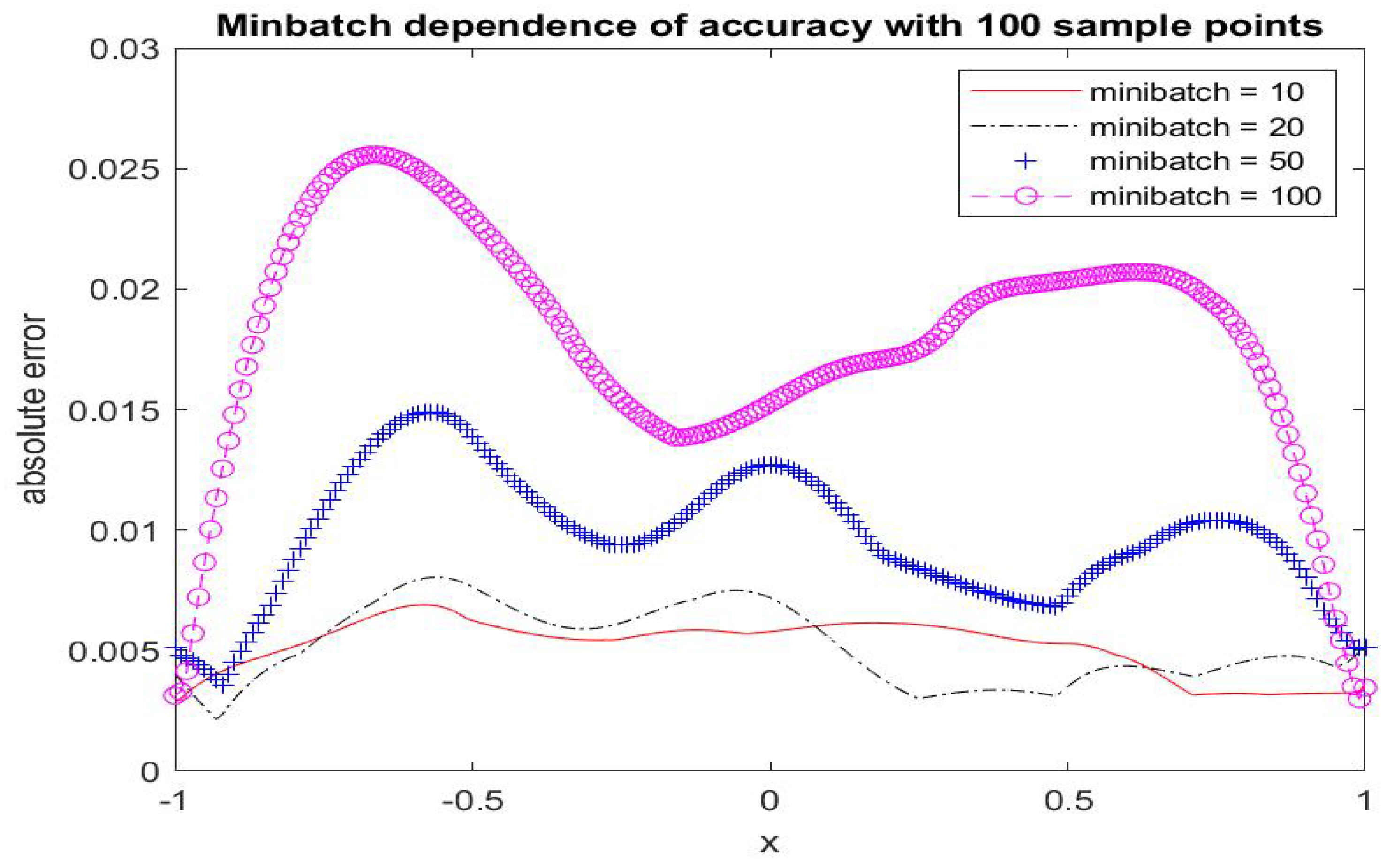
Figure 1.
Poiseuille flow: absolute error in u (comparison between the ALM-PINN and ALM solutions) in the case of 100 sample points with minibatch sizes 10, 20, 50 and 100. Setting and number of epochs .
Figure 1.
Poiseuille flow: absolute error in u (comparison between the ALM-PINN and ALM solutions) in the case of 100 sample points with minibatch sizes 10, 20, 50 and 100. Setting and number of epochs .
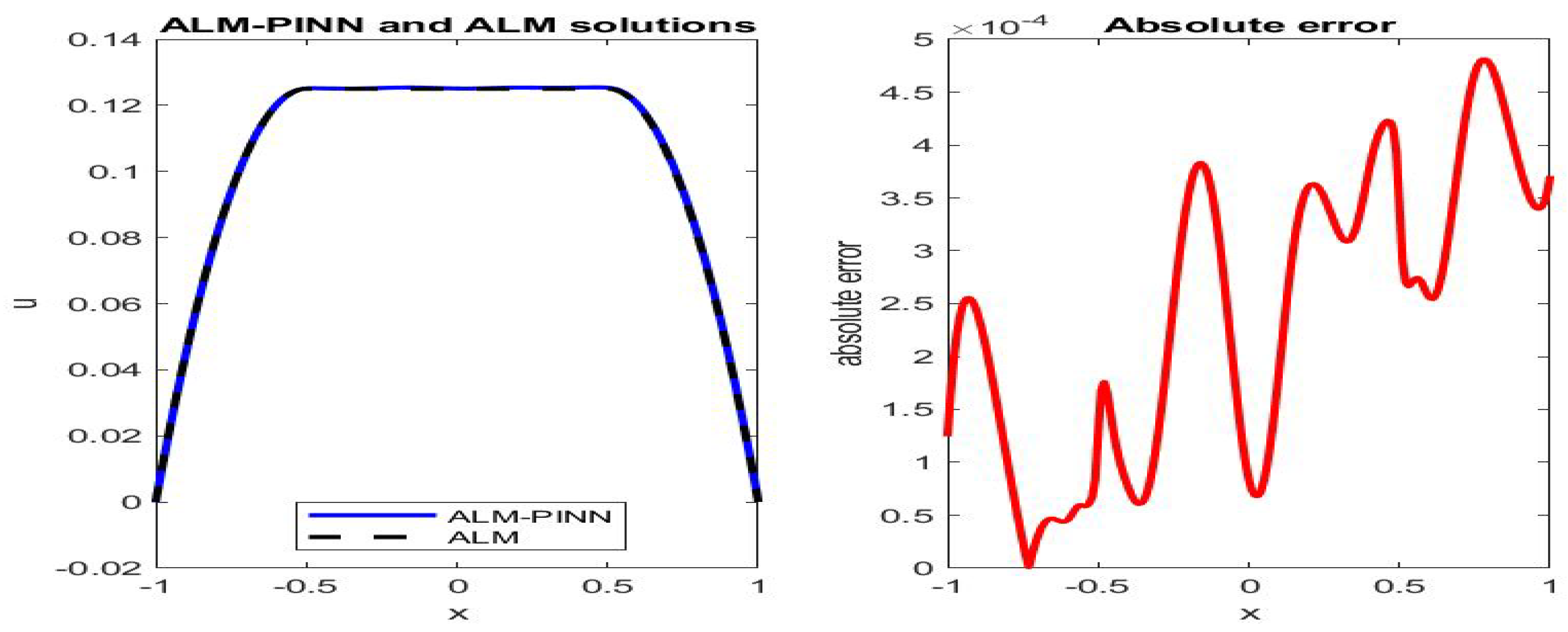
Figure 2.
Poiseuille flow: the ALM-PINN and ALM solution comparison (left), absolute error in u (right), in the case of 100 sample points with minibatch size 10. Setting and number of epochs .
Figure 2.
Poiseuille flow: the ALM-PINN and ALM solution comparison (left), absolute error in u (right), in the case of 100 sample points with minibatch size 10. Setting and number of epochs .
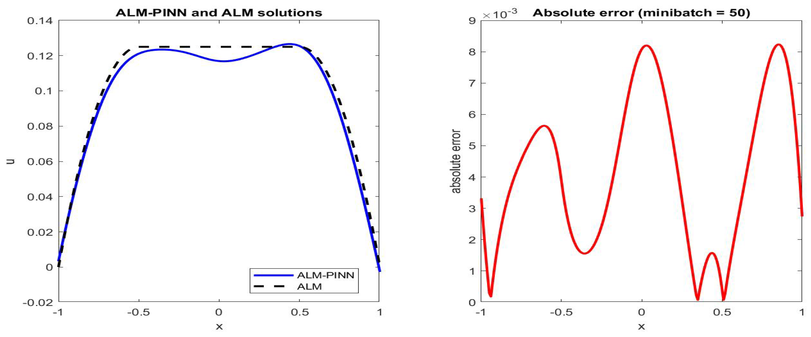
Figure 3.
Poiseuille flow: the ALM-PINN and ALM solution comparison (left), absolute error in u (right), in the case of 100 sample points with minibatch size 50. Setting and number of epochs .
Figure 3.
Poiseuille flow: the ALM-PINN and ALM solution comparison (left), absolute error in u (right), in the case of 100 sample points with minibatch size 50. Setting and number of epochs .
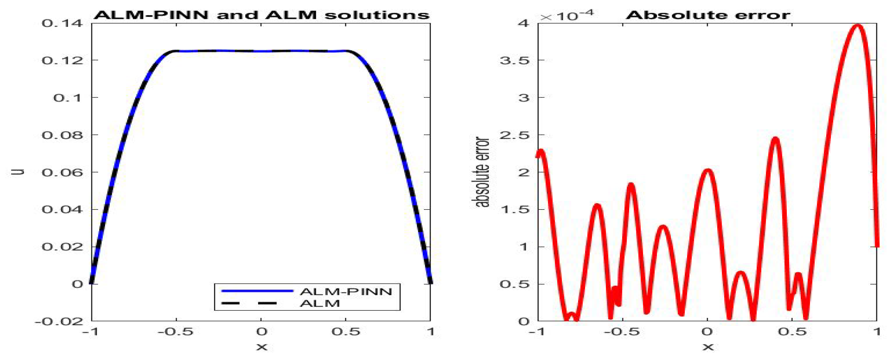
Figure 4.
Poiseuille flow: the ALM-PINN and ALM solution comparison (left), absolute error in u (right), in the case of 200 sample points with minibatch size 20. Setting and number of epochs .
Figure 4.
Poiseuille flow: the ALM-PINN and ALM solution comparison (left), absolute error in u (right), in the case of 200 sample points with minibatch size 20. Setting and number of epochs .
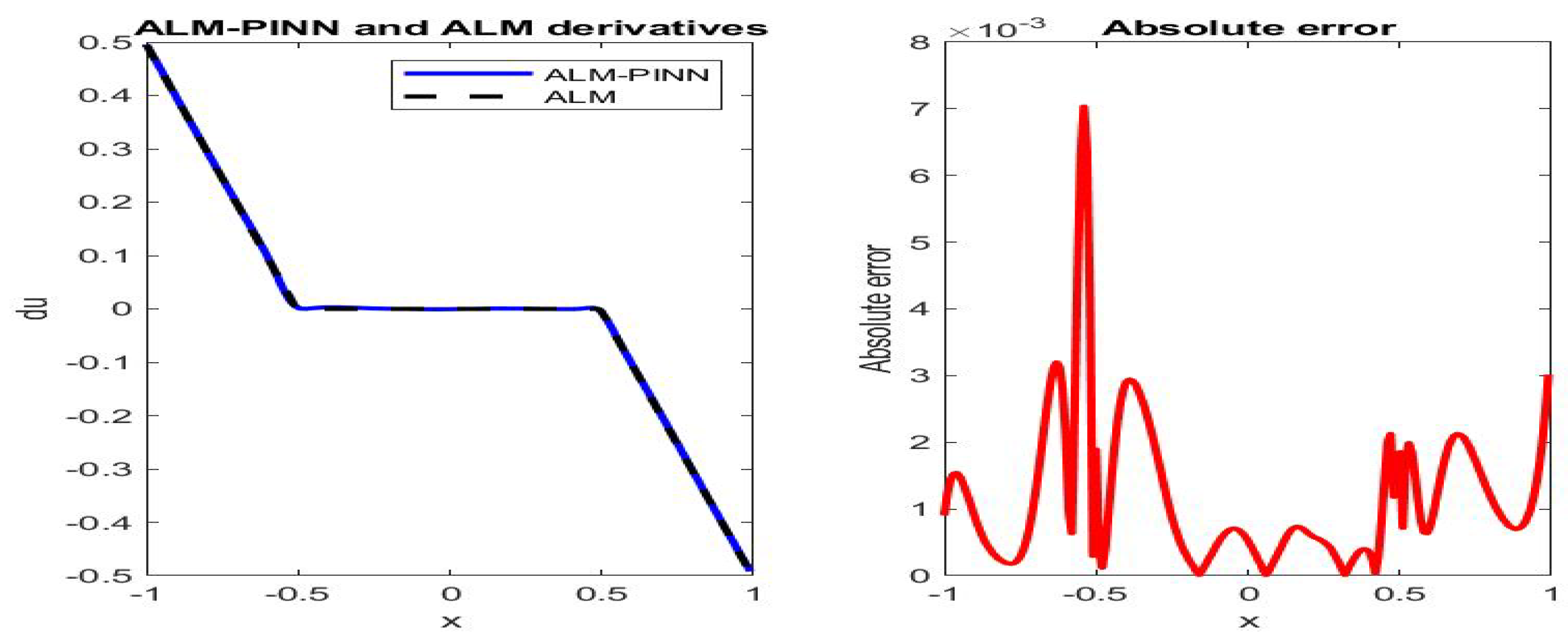
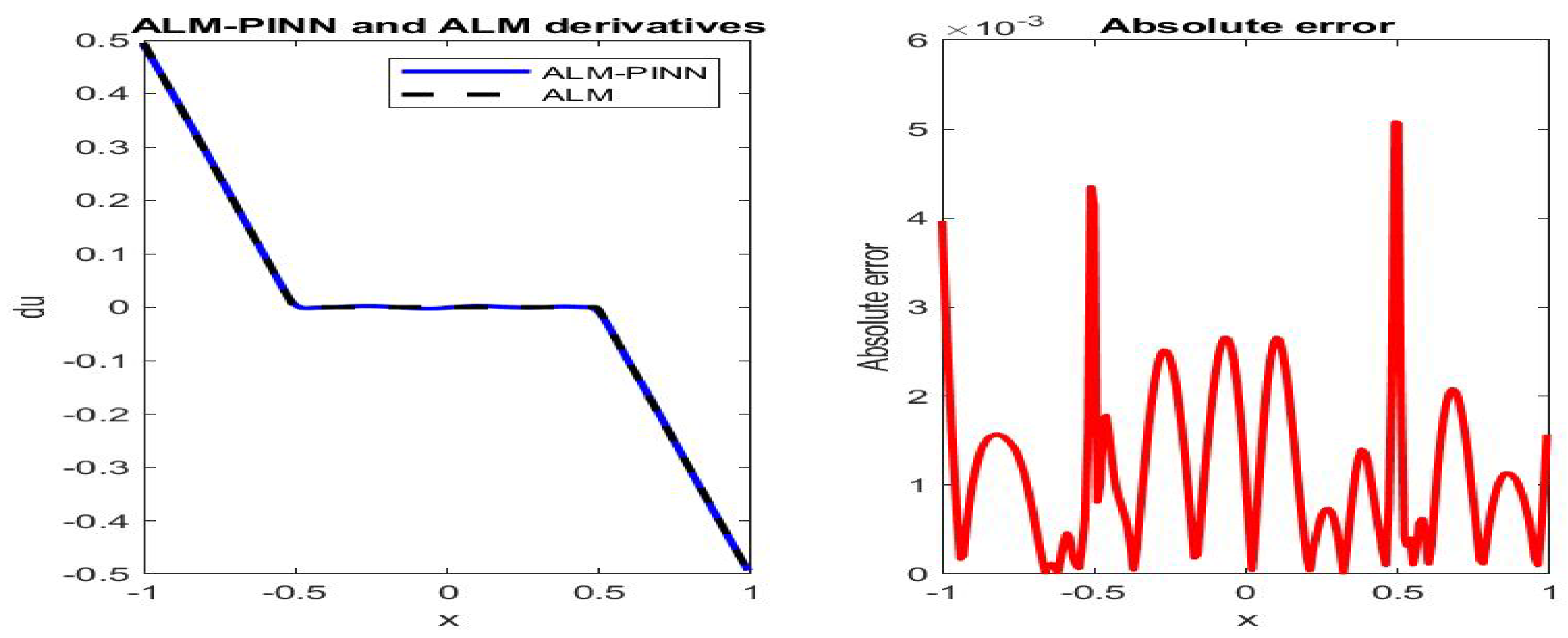
Figure 5.
Poiseuille flow: the ALM-PINN and ALM solution derivative comparison (left), absolute error in (right), in the case of 200 sample points with minibatch size 20. Setting and number of epochs .
Figure 5.
Poiseuille flow: the ALM-PINN and ALM solution derivative comparison (left), absolute error in (right), in the case of 200 sample points with minibatch size 20. Setting and number of epochs .
Figure 6.
Poiseuille flow: the ALM-PINN and ALM solution comparison (left), absolute error in u (right), in the case of 200 sample points with minibatch size 20. Setting , number of epochs , scaling factors and .
Figure 6.
Poiseuille flow: the ALM-PINN and ALM solution comparison (left), absolute error in u (right), in the case of 200 sample points with minibatch size 20. Setting , number of epochs , scaling factors and .
Figure 7.
Poiseuille flow: the ALM-PINN and ALM solution comparison (left), absolute error in u (right), in the case of 200 sample points with minibatch size 20. Setting , number of epochs , scaling factors and .
Figure 7.
Poiseuille flow: the ALM-PINN and ALM solution comparison (left), absolute error in u (right), in the case of 200 sample points with minibatch size 20. Setting , number of epochs , scaling factors and .
Figure 8.
Poiseuille flow: the ALM-PINN and ALM solution derivative comparison (left), absolute error in (right), in the case of 200 sample points with minibatch size 20. Setting , number of epochs , scaling factors and .
Figure 8.
Poiseuille flow: the ALM-PINN and ALM solution derivative comparison (left), absolute error in (right), in the case of 200 sample points with minibatch size 20. Setting , number of epochs , scaling factors and .
Figure 9.
Poiseuille flow: the ALM-PINN and ALM solution derivative comparison (left), absolute error in (right), in the case of 200 sample points with minibatch size 20. Setting , number of epochs , scaling factors and .
Figure 9.
Poiseuille flow: the ALM-PINN and ALM solution derivative comparison (left), absolute error in (right), in the case of 200 sample points with minibatch size 20. Setting , number of epochs , scaling factors and .
Figure 10.
Evolution of network learned (left) and (right) after 10, 100, 1000 and 8000 iterations, in the case of 200 sample points with minibatch size 20. Setting , number of epochs , scaling factors and .
Figure 10.
Evolution of network learned (left) and (right) after 10, 100, 1000 and 8000 iterations, in the case of 200 sample points with minibatch size 20. Setting , number of epochs , scaling factors and .
Figure 11.
Poiseuille flow: the ALM-PINN and ALM solution comparison (left), absolute error in u (right), in the case of 100 sample points on and extra 100 sample points on with minibatch size 20. Setting and number of epochs .
Figure 11.
Poiseuille flow: the ALM-PINN and ALM solution comparison (left), absolute error in u (right), in the case of 100 sample points on and extra 100 sample points on with minibatch size 20. Setting and number of epochs .
Figure 12.
Poiseuille flow: the ALM-PINN and ALM solution comparison (left), absolute error in u (right), in the case of 50 sample points on and extra 150 sample points on with minibatch size 20. Setting and number of epochs .
Figure 12.
Poiseuille flow: the ALM-PINN and ALM solution comparison (left), absolute error in u (right), in the case of 50 sample points on and extra 150 sample points on with minibatch size 20. Setting and number of epochs .
Figure 13.
Poiseuille flow: the ALM-PINN and ALM solution derivative comparison (left), absolute error in (right), in the case of 100 sample points on and extra 100 sample points on with minibatch size 20. Setting and number of epochs .
Figure 13.
Poiseuille flow: the ALM-PINN and ALM solution derivative comparison (left), absolute error in (right), in the case of 100 sample points on and extra 100 sample points on with minibatch size 20. Setting and number of epochs .
Figure 14.
Poiseuille flow: the ALM-PINN and ALM solution derivative comparison (left), absolute error in (right), in the case of 50 sample points on and extra 150 sample points on with minibatch size 20. Setting and number of epochs .
Figure 14.
Poiseuille flow: the ALM-PINN and ALM solution derivative comparison (left), absolute error in (right), in the case of 50 sample points on and extra 150 sample points on with minibatch size 20. Setting and number of epochs .
Figure 15.
Poiseuille flow: Solution error comparison (top) and derivative error comparison (bottom). Setting and number of epochs .
Figure 15.
Poiseuille flow: Solution error comparison (top) and derivative error comparison (bottom). Setting and number of epochs .
Figure 16.
Bingham number-dependent velocity profile of Poiseuille flow: Yield surfaces are captured by plotting contours of . The ALM-PINN learning is performed over 1000 interior points and boundary points, minibatch size 100 and number of epochs 10,000. The red solid lines represent the exact yield surfaces. The black solid lines are contour plots of at levels between and .
Figure 17.
Plots of pressure (left) and (right) at the lid for , and .
Figure 17.
Plots of pressure (left) and (right) at the lid for , and .
Figure 18.
Contour plots of network learned scaling factor for (left) and (right).
Figure 18.
Contour plots of network learned scaling factor for (left) and (right).
Figure 19.
Contour plots of network learned scaling factor for (left) and (right).
Figure 19.
Contour plots of network learned scaling factor for (left) and (right).
Figure 20.
Contour plots of network learned scaling factor for (left) and (right).
Figure 20.
Contour plots of network learned scaling factor for (left) and (right).
Figure 21.
Streamline and unyielded region plots in the lid-driven cavity of Bingham fluid with . (Left: solution from the Adam algorithm only. Right: solution after the LBFGS enhancement.)
Figure 21.
Streamline and unyielded region plots in the lid-driven cavity of Bingham fluid with . (Left: solution from the Adam algorithm only. Right: solution after the LBFGS enhancement.)
Figure 22.
Streamline and unyielded region plots in the lid-driven cavity of Bingham fluid with (left) and (right). Solutions are obtained via implementing the Adam algorithm and the LBFGS.
Figure 22.
Streamline and unyielded region plots in the lid-driven cavity of Bingham fluid with (left) and (right). Solutions are obtained via implementing the Adam algorithm and the LBFGS.
Table 2.
Key attributes of ALM-PINN.
Table 2.
Key attributes of ALM-PINN.
| Computational Aspects | Preferred Features of ALM–PINN |
|---|
| mesh requirements | mesh-free, flexibility of point sampling |
| formulation of solution | closed-form available, easy to evaluate |
| in higher dimensions | more cost-effective vs. mesh-based methods |
| time dependent problems | one network training, no stability concerns |
| parameter dependent solutions | one network training, cost-effective |
| ALM convergence | enhanced by adaptive weights |
| stream function formulation | divergence free constraint eliminated |
| loss function | feasible for network training |
Table 3.
Comparison of the proposed ALM-PINN to other approaches.
Table 3.
Comparison of the proposed ALM-PINN to other approaches.
| Methods | Objective Functions | Handling Singularity |
|---|
| ALM | + I + II | + regularization term (RT) |
| | | RT of fixed scale |
| | | slow convergence |
| | | fine meshes required |
| modified ALM | + I + II | + penalization term (PT) |
| | | PT allowed |
| | | relatively faster convergence |
| | | fine meshes required |
| PINNs | Loss function | Bingham fluids |
| | (from BVP) | (no explicit PDEs) |
| | | ⇒ not applicable |
| | | mesh-free |
| weight adaptivity | Loss function | |
| ([48]) | (from BVP or AL) | network learned weights: |
| | | constant |
| ALM-PINN | Loss function | + RT scaled via DAW |
| (new DAW) | ( + II + BCs) | convergence adjusted by network |
| | | built-in divergence free |
| | | (stream function formulation) |
| | | mesh-free |
| | | user specified |
| | | hyperparameters: |
| | | (Fixed) |
| | | network learned weights: |
| | | scaling function |
Table 4.
The ALM-PINN performance comparison for different B values.
Table 4.
The ALM-PINN performance comparison for different B values.
| B | | Vortex Center | Loss | loss | Loss | Loss |
|---|
| 2 | 250 | | | | | |
| 5 | 1000 | | | | | |
| 20 | 2500 | | | | | |
Table 5.
Poiseuille flow (B-dependent solution): convergence of ALM-PINN with respect to network depth (number of layers ) and width (number of neurons in each hidden layer). Activation function is tanh, with 1000 sample points, and after 10,000 epochs. No weight adaptivity.
Table 5.
Poiseuille flow (B-dependent solution): convergence of ALM-PINN with respect to network depth (number of layers ) and width (number of neurons in each hidden layer). Activation function is tanh, with 1000 sample points, and after 10,000 epochs. No weight adaptivity.
| | Loss | Loss | Loss |
|---|
| 4 | 20 | | | |
| | 30 | | | |
| 5 | 20 | | | |
| | 30 | | | |
| 6 | 20 | | | |
| | 30 | | | |
Table 6.
Driven cavity (): convergence of ALM-PINN with respect to network depth (number of layers ) and width (number of neurons in each hidden layer ). Activation function is tanh, with 60,000 sample points, and after 14,000 epochs. Boundary hyperparameter , with weight adaptivity and .
Table 6.
Driven cavity (): convergence of ALM-PINN with respect to network depth (number of layers ) and width (number of neurons in each hidden layer ). Activation function is tanh, with 60,000 sample points, and after 14,000 epochs. Boundary hyperparameter , with weight adaptivity and .
| | Loss | Loss | Loss | Loss |
|---|
| 5 | 30 | | | | |
| | 40 | | | | |
| 6 | 30 | | | | |
| | 40 | | | | |
| 7 | 30 | | | | |
| | 40 | | | | |
Table 7.
Poiseuille flow (B-dependent solution): convergence of the Adam algorithm without weight adaptivity (left) and with weight adaptivity (right). Activation function is tanh, with 1000 sample points, and after 2000, 40,000, 6000, 8000 epochs.
Table 7.
Poiseuille flow (B-dependent solution): convergence of the Adam algorithm without weight adaptivity (left) and with weight adaptivity (right). Activation function is tanh, with 1000 sample points, and after 2000, 40,000, 6000, 8000 epochs.
| Steps | Loss | Loss | Loss |
|---|
| 2000 | 6.412; 3.979 | 6.125; 2.651 | 1.722; 1.599 |
| 4000 | 5.138; 1.234 | 3.120; 0.997 | 1.573; 1.091 |
| 6000 | 1.817; 1.011 | 1.047; 0.766 | 1.432; 1.584 |
| 8000 | 1.536; 0.652 | 1.072; 0.503 | 1.260; 1.013 |
Table 8.
Driven cavity (): convergence of the Adam algorithm with weight adaptivity and , boundary hyperparameter . Activation function is tanh, with 60,000 sample points, and after 2000, 40,000, 6000, 8000, 10,000 epochs.
Table 8.
Driven cavity (): convergence of the Adam algorithm with weight adaptivity and , boundary hyperparameter . Activation function is tanh, with 60,000 sample points, and after 2000, 40,000, 6000, 8000, 10,000 epochs.
| Steps | Loss | Loss | Loss | Loss |
|---|
| 2000 | | | | |
| 4000 | | | | |
| 6000 | | | | |
| 8000 | | | | |
| 10,000 | | | | |
Table 9.
Driven cavity (): convergence of the Adam algorithm with weight adaptivity and , boundary hyperparameter . Activation function is tanh, with 60,000 sample points, and after 2000, 40,000, 6000, 8000, 10,000 epochs.
Table 9.
Driven cavity (): convergence of the Adam algorithm with weight adaptivity and , boundary hyperparameter . Activation function is tanh, with 60,000 sample points, and after 2000, 40,000, 6000, 8000, 10,000 epochs.
| Steps | Loss | Loss | Loss | Loss |
|---|
| 2000 | | | | |
| 4000 | | | | |
| 6000 | | | | |
| 8000 | | | | |
| 10,000 | | | | |


