Article

Machine-Learning Classification Models to Predict Liver Cancer with Explainable AI to Discover Associated Genes

1
Department of Mathematical Sciences, The University of Texas at El Paso, El Paso, TX 79968, USA
2
Department of Mathematics and Statistics, Texas Tech University, Lubbock, TX 79409, USA
3
Department of Mathematics and Computer Sciences, Southern Arkansas University, Magnolia, AR 71730, USA
*
Authors to whom correspondence should be addressed.
AppliedMath 2023, 3(2), 417-445; https://doi.org/10.3390/appliedmath3020022
Submission received: 16 February 2023 / Revised: 3 April 2023 / Accepted: 24 April 2023 / Published: 12 May 2023

Abstract

:
Hepatocellular carcinoma (HCC) is the primary liver cancer that occurs the most frequently. The risk of developing HCC is highest in those with chronic liver diseases, such as cirrhosis brought on by hepatitis B or C infection and the most common type of liver cancer. Knowledge-based interpretations are essential for understanding the HCC microarray dataset due to its nature, which includes high dimensions and hidden biological information in genes. When analyzing gene expression data with many genes and few samples, the main problem is to separate disease-related information from a vast quantity of redundant gene expression data and their noise. Clinicians are interested in identifying the specific genes responsible for HCC in individual patients. These responsible genes may differ between patients, leading to variability in gene selection. Moreover, ML approaches, such as classification algorithms, are similar to black boxes, and it is important to interpret the ML model outcomes. In this paper, we use a reliable pipeline to determine important genes for discovering HCC from microarray analysis. We eliminate redundant and unnecessary genes through gene selection using principal component analysis (PCA). Moreover, we detect responsible genes with the random forest algorithm through variable importance ranking calculated from the Gini index. Classification algorithms, such as random forest (RF), naïve Bayes classifier (NBC), logistic regression, and k-nearest neighbor (kNN) are used to classify HCC from responsible genes. However, classification algorithms produce outcomes based on selected genes for a large group of patients rather than for specific patients. Thus, we apply the local interpretable model-agnostic explanations (LIME) method to uncover the AI-generated forecasts as well as recommendations for patient-specific responsible genes. Moreover, we show our pathway analysis and a dendrogram of the pathway through hierarchical clustering of the responsible genes. There are 16 responsible genes found using the Gini index, and CCT3 and KPNA2 show the highest mean decrease in Gini values. Among four classification algorithms, random forest showed 96.53 % accuracy with a precision of 97.30 % . Five-fold cross-validation was used in order to collect multiple estimates and assess the variability for the RF model with a mean ROC of 0.95 ± 0.2 . LIME outcomes were interpreted for two random patients with positive and negative effects. Therefore, we identified 16 responsible genes that can be used to improve HCC diagnosis or treatment. The proposed framework using machine-learning-classification algorithms with the LIME method can be applied to find responsible genes to diagnose and treat HCC patients.

1. Introduction

HCC is the most common liver cancer and the fastest growing cause of cancer-related death in the United States.
HCC causes more than 85 percent of all primary liver cancers. It is the sixth most prevalent cancer worldwide and the second leading factor in cancer-related fatalities [1]. The high mortality rate of HCC results from metastasis or the development of newly generated tumors within the diseased liver. Research has revealed that 90% of all cancer-related fatalities are caused by metastasis [2].
Since HCC’s genome sequence changes over time and the gene expression patterns are so diverse among patients, it is nearly impossible to pinpoint the mechanisms and pathways of the disease. This is why ineffective therapy is to blame for poor patient outcomes in the HCC patient group. Recurrence after surgery is a major factor in HCC’s poor prognosis, and there are currently few therapeutic approaches that successfully reduce recurrence due to metastasis. In the clinical setting, one of the difficulties is in identifying HCC patient subgroups at high risk of developing metastatic illness in advance.
The efficacy of a metastatic signature made up of 153 genes that might identify HCC patients as a risk classifier for HCC recurrence and survival was examined using two independent cohorts totaling 386 HCC patients [3]. There are insufficient significant machine learning-based studies to predict HCC in the early stages of cancer development. We aimed to discover the HCC-causing genes so that medical professionals could take the necessary precautions to stop HCC in its early stages of development.
According to the conventional tumor evolution model, a primary tumor is initially benign but develops mutations over time, allowing a small number of tumor cells to spread. To enhance patient survival, early diagnosis of tumors that have already mutated is extremely important. Using genes whose copy counts correspond with gene expression and cancer development as the standard for HCC driver genes, Roessler et al. employed an integrated strategy to find these genes, even though the mechanisms underlying the aggressive cancer HCC genesis and progression are poorly understood [4]. This study directed us to apply state-of-the-art artificial-intelligence techniques to determine the responsible genes for developing HCC.
Although surgical resection and liver transplantation are possible, the recurrence rate is significant. Furthermore, surgery is usually out of the question since the disease has progressed too far. Given these patients with HCC, especially those incompetent for surgical resection or liver transplant, it is crucial to identify the key drivers and potential treatment targets [5]. Zhao et al. showed the viability and strength of a novel approach by identifying key pathways associated with prognostically significant HCC subtypes using well-defined patient samples and integrated genomics [4], in this study, they used clustering algorithms to find the key pathways. This can be improved significantly by applying the machine-learning algorithms to high dimensional genomics data to determine the key genes that cause the HCC disease.
It is common practice to extract a biological sample and then use microarrays to express the genes; however, this is not the approach used in our study. Statistical approaches are used to assess the data and discover meaningful content that biologists can utilize to give them biological significance once the data have been transformed into numbers. Numerous genome-wide tools, including microarrays and, more recently, next-generation sequencing platforms, have been used to analyze thousands of clinical HCC samples in an effort to identify promising treatment targets [5].
Moreover, there are minimal applications of machine-learning methods in genomics datasets for identifying the key genes responsible for HCC apart from bioinformatic analysis. Wang et al. discovered 13 clinically significant target genes with therapeutic promise utilizing genome-wide growth-depletion screens and combining real HCC tumor expression data and clustered, regularly spaced, short palindromic repeats [6]. Thus, there is a great possibility to discover significant target genes by applying machine-learning algorithms in addition to bioinformatics analysis.
Lu et al. investigated Numb mRNA expression in tumors and surrounding healthy tissues using either χ ˜ 2 or Mann-Whitney U-tests on a microarray dataset of 241 HCC patients to determine the relationship between clinicopathological traits and HCC subtypes [7].
In this case, machine-learning methods could be very useful for analyzing a high-dimensional dataset to determine additional marker genes that cause HCC. A microarray is a type of experimental setup where probes are created or attached to solid substrates to expose them to the target molecules. The microarray dataset holds experimental data in a matrix, where the columns typically correspond to sample IDs, and the rows correspond to the names of genes or probes.
Microarray genomic data analysis is useful for finding differentially expressed long non-coding RNA (lncRNA). According to Chen et al.’s bioinformatic analysis of liver tissue in brain-dead donor liver transplantation, microarray probes effectively identified hundreds of transcripts by displaying differentially expressed lncRNA and circRNA profiles [8]. Thus, using machine-learning techniques, we may decipher nuanced connections and identify intricate patterns in microarray data. To better understand diseases and discover treatments, medical researchers use the analysis of microarrays and gene expression. Particularly complex disorders, such as HCC, might be the subject of significant knowledge.
Due to its poor prognosis and ineffective response to systemic therapy, HCC ranked fourth among the top causes of cancer-related fatalities in 2018. Considering this situation, the HCC survival rate is still below tolerable levels. It is essential to continue looking for possible HCC prognostic and therapeutic targets by improving our comprehension of the cellular biological processes [9]. The genetic machinery responsible for metastasis is hard-wired into tumors from the start, which motivates tumor profiling to forecast patient progress.
Gene ontology is an area of study where we investigate the roles of genes and proteins in cells [10]. Pathway-analysis techniques are used in bioinformatics to find important genes/proteins within a previously known pathway in connection to a certain experiment or pathogenic state. Pathway analysis is a common technique to understand and analyze biological data, such as gene datasets. This is a useful tool that is based on the collection and use of knowledge that includes biomolecular functioning, as well as statistical testing and other algorithms [11]. Moreover, methods of pathway analysis assist cancer researchers in determining the biological roles of genes and gene sets inside malignant tissues [12].
Machine-learning techniques have lately become more precise and effective compared with conventional parametric algorithms when used for large area modeling and working with high-dimensional and complex datasets [13,14,15]. Since these algorithms do not rely on data distribution assumptions, such as normality, they are more accurate, efficient, and effective [16,17]. For two class situations, recent research showed that random forests are equal to a kernel operating on the true margin in distribution space [18]. The symmetry of the kernel is said to be enforced by randomness (poor correlation), while strength increases a desirable skewness at abruptly curved boundaries. This should clarify the dual functions of correlation and strength. Understanding may also be aided by [19]’s theoretical framework for stochastic discrimination.
Santos et al. employed logistic regression and neural network classifiers to classify the 165 patients in the Coimbra Hospital and University Centre database, with NN achieving an accuracy of 75.2% and LR achieving 73.3% [20]. Proper preprocessing of the dataset might considerably enhance their model to achieve better accuracy. Thus, we focused on the data pre-processing to obtain better accuracy in our developed models. Acharya et al. introduced a hybrid system that used three algorithms, including linear discriminant analysis to minimize the number of features, a support vector machine (SVM) for classification, and a genetic algorithm to improve the model, and produced accuracy of 90.30%, specificity of 96.07%, and sensitivity of 82.25% [21].
Muflikhah et al. proposed a unitary singular matrix feature selection approach for facilitating hepatoma detection and classification. To calculate the pattern k-rank, the feature was deconstructed using a single vector. They applied several machine-learning algorithms, including KNN, naïve Bayes, decision tree, and SVM, and the experimental outcome had an AUC of above 90% [22].
To achieve the best HCC detection accuracy, Ksia̧żek et al. developed a unique machine-learning model that uses seven classifiers in a stacking learning (ensemble) manner, including KNN, random forest, naïve Bayes, and four additional classifiers. The maximum accuracy and F 1 -score were reached by their suggested approach at 0.9030 and 0.8857, respectively, [23].
The random forest classifier has been tested against the NBC, logistic regression, and k-NN classifiers. It is based on probability models with strong assumptions of independence. NBC models are created using Bayes’ theorem. Despite their simple design and assumptions, naïve Bayes classifiers [24] have performed excellently in various challenging real-world settings. However, a comprehensive comparison with different classification algorithms in 2006 revealed that more advanced methods, such as boosted trees or random forest, outperformed Bayes classification.
The naïve Bayes classifier [25] model was employed to determine if it yielded the same conclusions as the gene expression data. The random forest method does not require the researcher to propose any particular model structure. This is essential in early genome-wide or candidate-area prospective studies where the feature’s genetic structure is ambiguous. However, combining a vast number of genes and relatively small microarrays introduces new challenges for statistical models. They are also gaining popularity because of their extensive use in microarray data analysis with the capacity to handle numerous genes without using traditional feature selection and in having robustness to outliers.
Models must be understandable by users if humans are to trust AI technologies. AI interoperability sheds light on what is happening inside these systems and aids in the detection of potential problems, including causality, information leakage, model bias, and robustness. The concept comes from a work published in 2016 by the title “Why should I trust you?”, referring to explaining the predictions of any classifier [26] in which the researchers perturbed the initial data points, fed them into the black box model, and watched what happened.
The approach then adjusted the weights of those additional data points based on how close they were to the original point. It used those sample weights to fit a substitute model, such as linear regression, to the dataset with variations. The newly trained explanation model can then be used to explain each original data point. Local interpretable model-agnostic explanations (LIME) provide a general framework to decipher black boxes and explain the “why” behind forecasts or suggestions made by AI. LIME was studied by many researchers for improving diagnoses of patients [27,28,29].
In this study, we are interested in how doctors and patients can trust machine-learning prediction when each patient is different from the other, and when multiple parameters can decide between HCC or not. To solve this problem, LIME was used in the test model. The method of explanation should be applicable to all ML models. We use this as an explanation that is model-agnostic along with the individual predictions, and the model should be explainable in its entirety, i.e., a global perspective was considered. In the past, researchers have not conducted any studies for the HCC microarray dataset. There are a few studies that exist for the classifications of liver cancers, but they are not related to AI explanations.
Foremost, a comprehensive and proficient framework for the gene expression data of HCC is proposed in this article. The classification accuracy of ML models among different classification algorithms is used to determine which model is the best among them. The trained model then passes through an AI-explainable approach. We applied existing algorithms using the HCC gene dataset and proposed an effective framework. Under the current framework used in the present study, no one has considered this gene expression data of HCC with ID GSE14520 [30].
In brief, we want to find patterns in the gene changes to assess whether they are normal or indicative of HCC disease. To select the important variables, we use the Gini index and entropy with information. To visualize and reduce dimensionality, a heat map, and principal components are used. ROC and biostatistical analyses are reported to compare model validity.
LIME is used to interpret the responsible genes for a particular HCC patient. Biological references are included with rigorous literature reviews to examine connections between genes and the disease. Pathway analysis is shown to present the clusters of genes with their biological importance in HCC prediction.

2. Methodology and Framework

2.1. Samples from Gene Data

Data were collected from the National Center for Biotechnology Information (NCBI). The title of the dataset is Gene Expression Data of HCC with ID GSE14520 [30], and the access date of this gene expression dataset was 1 March 2022. To study the gene expression patterns in HCC patient tumors and non-tumor tissue matched with healthy donor liver tissue, Affymetrix microarray profiling was used by lab technicians. Using a single channel array technology, tumors and matching non-tumor tissues were assessed independently for gene expression profiling.
On Affymetrix GeneChip HG-U133A 2.0 arrays, data providers used the manufacturer’s instructions to evaluate tumor and non-tumor samples from 22 patients in cohort 1 as well as normal liver samples. They measured the fluorescence intensities using GCOS Affymetrix software and an Affymetrix GeneChip Scanner 3000. On the 96 HT HG-U133A microarray platform, all samples from cohort 2 as well as 42 tumors and paired non-tumor samples from cohort 2 were processed. Thus, we extracted the gene expression microarray data GSE14520 from the NCBI GEO website.
Four hundred forty-five samples were taken from patients between 2002 and 2003 at the Liver Cancer Institute (LCI), Fudan University in China, and the Liver Tissue Cell Distribution System (LTCDS), the University of Minnesota in the United States. The dataset contained 222 cases and 212 controls; however, no case-control data were provided for 11 cases. The majority of HCC patients had a history of hepatitis B infection (96.31%).

2.2. Mathematical Framework Machine-Learning Approaches

For mathematical framework, we use the methodology in the diagram of Figure 1. Let us consider that the predictor gene data matrix is X R n x r and the target/response variable is T R r . The prepossessed microarray dataset was retrieved from the NCBI GEO repository and cleaned using R software’s LIMMA package and Bio conductor [31]; the version and description of the package are given in Appendix A.1. The dimensions of this dataset are 445 by 22,268, with 445 samples and 22,268 genes. Additionally, of the dataset’s 46 phenotypic features, tumor and non-tumor tissue types are employed as response variables and are factorized into 0 and 1 to facilitate the analysis.
The dataset was additionally cleaned to eliminate any “NA”, which means not available in the data point, and a response variable column was added to the gene dataset along with sample ID matching between the phenotypic dataset and the gene dataset. This dataset was used for machine learning and statistical analysis to predict HCC. Four different classification methods were used. These were random forest, naïve Bayes classifier, k-NN, and logistic regression. We showed the final results in the form of plots, such as a confusion matrix, and ROC analysis was compared to obtain the results.

2.3. Variable Selection for Classification, Pathway Analysis, and Statistical Analysis

2.3.1. Dimension Reduction and HCC Gene Mining

PCA is the process of transforming high-dimensional data into an orthogonal basis in such a way that the first principal component (PC) is aligned with the source of variance that contributes the most variation. The second PC is aligned with the source of variance that contributes the most variation that remains, and so on. After this, high-dimensional data are now more suitable for visual investigation, since we are able to investigate projections on the first two (or few) PCs. The samples’ PC scores serve as the coordinates on the new PC axis.
The eigenvalue for a given principal component measures the amount of that PC’s explained variance. Using this, we can determine how much of the total variation in the initial data is explained by each axis. Each variable’s “weight” on a given PC is represented by its variable loading (eigenvector). These may be seen as the relationship that exists between the principal component and the underlying variable.
In statistical software R, the prcomp() function is used to calculate a PCA. This function requires a data matrix, with columns containing the variables that will be used to transform the samples. In this study, we are interested in comparing the gene expression levels among samples to find similarities. As a result, we must provide the prompt() method with a transposed version of the data. By using prcomp(), we are able to determine the percentage of total variation that is explained by each PC in our dataset.
Finally, we investigate which genes have the largest impact on each PC axis. This data can be found in the prcomp() object’s rotational value, which represents the PCA’s variable loadings. Mathematically, r-dimensional data matrix X R n x r and new lower dimension is d < < r , mean X ¯ = 1 n n = 1 n x i , and the covariance is Σ x = 1 n n = 1 n ( x i x i ¯ ) ( x i x i ¯ ) T . Then, we find the spectral decomposition of Σ x is Σ x = Q Λ Q 1 , where the eigenvectors are { q 1 , q 2 , , q r } , and their corresponding eigenvalues are λ 1 , λ 2 , , λ r . Therefore, with singular value decomposition, the sorted eigenvalues in lower dimension λ 1 λ 2 , λ d . Thus, the lower dimensional representation of the microarray HCC dataset is as follows,
y = ( λ 1 T ( x x ¯ ) λ 1 , λ 2 T ( x x ¯ ) λ 2 , , λ d T ( x x ¯ ) λ d ) T R d
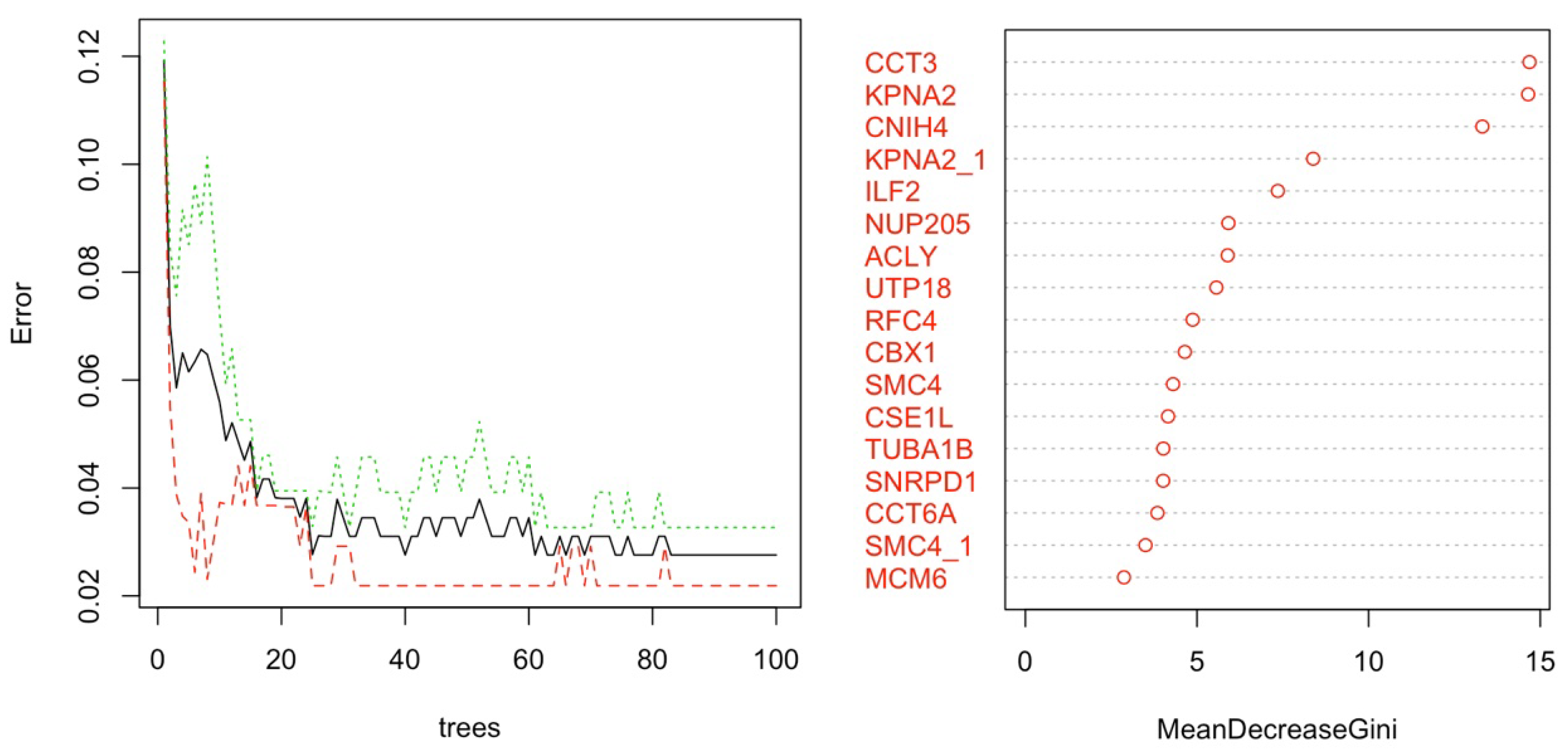
Since all 22,269 genes are not responsible for HCC, and there might be multicollinearity in the features, we instead focused on the top 100 genes (Figure 2) in terms of PC loading. To identify the most 100 important variables/genes, the above PCA technique [32,33] was employed. The top 17 genes were obtained from variable importance ranking [34]. Moreover, random forest was used for classification, and RF was the average of multiple decision trees.
As a result, the following discussions were incorporated into the framework. The datasets must first be divided into parts in order to form an intermediate decision tree with root nodes at the top, which is fundamental to decision trees. Then, the decision tree’s stratification model leads to the final result through the tree pass-over nodes. A comprehensive discussion of the entropy, Gini index, and information gain, as well as their roles in the decision tree method implementation, may be found here [35,36].
Furthermore, because many factors influence decision making, the significance and impact of each factor must be studied. The root node is assigned as the required feature, and the node division is traversed downwards. At each node, descending downward reduces impurity and uncertainty levels, resulting in enhanced classification or an exclusive split. Splitting measures, such as entropy, information gain, and the Gini index have been used to solve the problem. Entropy quantifies the impurity or randomness of data points.
It is a value between 0 and 1. Entropy close to 1 indicates that the model has a higher level of disorder. The concept of entropy is crucial for computing information gain. By determining which feature provides the most information about the classification based on the idea of entropy, information gain is used to determine which feature provides the most information about the classification, with the goal of reducing the amount of entropy starting from the top (root node) to the bottom (leaves nodes). Mathematically, entropy is defined as follows:
Entropy = k = 1 n p k log 2 ( p k ) ,
where p k denotes the probability that it is a function of entropy. The Gini index is defined as follows: The Gini index ranges from 0 to 1. A Gini index of 0 corresponds to absolute classification, meaning that all of the items belong to a single class or that only one class is present. A Gini index of 1 shows the uneven distribution of components across several categories. A Gini index of 0.5 indicates that items in some classes are distributed equally. The Gini index can be represented mathematically as:
Gini Index = k = 1 n P k 2 ,
where P k is known as the chance that an element will be assigned to a specific class. Each feature’s importance is determined by the Gini importance or mean decrease in impurity (MDI) method, which adds up all of the splits (across all trees) that include the feature in proportion to the number of samples it splits. This idea was used in the RF algorithm after discussing the other classification algorithms below.

2.3.2. Classification of Gene Expression Data

Four different machine-learning techniques are applied to classify HCC from the gene expression data. The foremost technique is the naïve Bayes Classifier, which is asymptotically equivalent to logistic regression if the naïve Bayes assumption holds. Another well-known technique is the k-nearest neighbor (k-NN) classifier. The Euclidean distance between the test and training samples is used as the basis for the k-NN determination of the class level for the test samples.
For microarray profiling, gene expression patterns in healthy donor livers, as well as tumor and paired non-tumor tissue from HCC patients, were analyzed. k-NN classifies whether it is a tumor and paired non-tumor tissue of HCC patients or not based on the Euclidean distance. Finally, the random forest method is applied, and its result is produced from the aggregation of the decision trees.

Naïve Bayes Classifier for HCC Classification:

Although the naïve Bayes classifier is not linear in general, it corresponds to a linear classifier in a given feature space provided the probability likelihood factors p ( t i | c ) come from exponential families. In this instance, the information is based on HCC, and the label is either cancer or not. The naïve Bayes assumption states that the variables in the data are conditionally independent, both liver cancer and non-liver cancer are picked independently at random regardless of whether we are aware that a patient has cancer. Although this assumption can be fragmented, the resulting classifiers can still perform well in real-world applications [37,38]. Let us assume the naïve Bayes assumption holds for now and define the Bayes classifier by:
h ( x ) = argmax P ( t | x ) = argmax P ( x | t ) P ( t ) P ( x ) = argmax P ( x | t ) P ( t ) = argmax α = 1 d P ( x α | t ) P ( t ) = argmax α = 1 d log ( P ( x α | t ) ) + log ( P ( t ) ) .
One dimension estimating log ( P ( x α | t ) ) should be considered because it is easy to calculate. Now, suppose that t i ( 1 , + 1 ) and that the features are multinomial. The goal is to show that
h ( x ) = argmax P ( t ) α 1 d P ( x α | t ) = sign ( w T x + b ) ,
that is,
w T x + b > 0 h ( x ) = + 1 .
Since P ( x α | t = + 1 ) θ α + x α and P ( T = + 1 ) = π + :
W α = log ( θ α + ) log ( θ α ) , b = log ( π + ) log ( π )
One can compute the w T x + b by applying the above for performing classification. By further simplification,
w T x + b > 0 ,
which implies
α = 1 d x α ( log ( θ α + ) log ( θ α ) + log ( π + ) log ( π ) ) > 0 ,
e x p ( α = 1 d x α ( log ( θ α + ) log ( θ α ) + log ( π + ) log ( π ) ) > 1
α = 1 d e x p ( log ( θ α + x α ) + log ( π + ) ) e x p ( log ( θ α x α ) + log ( π ) ) > 1 α = 1 d ( θ α + x α π + ) ( θ α x α π ) > 1
α = 1 d P ( x α | T = + 1 ) π + α = 1 d P ( x α | T = 1 ) π > 1 P ( x | T = + 1 ) π + P ( x | T = 1 ) π > 1 P ( T = + 1 | x ) P ( T = 1 | x ) > 1
P ( T = + 1 | x ) > P ( T = 1 | x ) argmax P ( T = t | x ) = + 1 .
If naïve Bayes predicts + 1 , this demonstrates that point x is located on the positive side of the hyperplane. Note that, in this paper, tumor and non-tumor tissue types are employed as response variables and are factorized into 0 and 1 to facilitate the analysis. In this gene expression dataset, all the variables are continuous; therefore, Gaussian naïve Bayes can be considered. As a result, if the naïve Bayes hypothesis is true, both the naïve Bayes classifier and the logistic regression generate asymptotically identical models.
Moreover, NBC is fast and simple to implement, works well with high-dimensional datasets, requires a relatively small amount of training data, and can handle both continuous and discrete data. It also assumes independence between features, which is rarely true in real-world scenarios. On the other hand, logistic regression is simple to implement, works well with small to medium-sized datasets, and outputs a probability score that can be interpreted. However, it requires careful feature selection and may not perform well with non-linear data.

Logistic Regression Classifier for HCC Classification:

The logistic regression model is used to model the relationship between a binary target variable and a set of independent variables. In logistic regression, the model predicts the logistic regression transformation of the probability of the event, which is used for the high dimensional gene expression data [39]. The following mathematical formula is used to generate the final output:
t i = logit P i 1 P i = b 0 + b 1 x 1 + b 2 x 2 + + b n x n .
The odds ratio is represented by P i in the equation above, and its formula is as follows:
o d d s = P i 1 P i ,
where P i stands for the probability of “presence of HCC”, and 1 P i is for the “absence of HCC”. The predicted values from the above model, the log odds of the event, can be transformed into the probability of an event as follows:
P i = 1 1 1 + e t i .
In matrix–vector form, t i = b 0 + b T X . Then, ( b 0 , b 1 , , b n ) is fitted through the maximum likelihood estimator. Then, the log-likelihood function is l ( b 0 , b ) = i = 1 d log ( P ( T = t i | X = x i ) ) . Therefore,
( b 0 ^ , b ^ ) = argmax i = 1 d log ( t i ( b 0 + b T x i ) ) log ( 1 + e x p ( b 0 + b T x i ) ) .
Another well-known classifier is the k-nearest neighbor classifier, which depends on a distance metric [40,41]. The more accurately the metric captures label similarity, the more accurately the classification is determined. k-NN is discussed in the next subsection. k-NN is non-parametric and flexible, can handle both regression and classification problems, and is simple to understand and implement. It can be computationally expensive, sensitive to irrelevant features and noisy data, and requires tuning of hyperparameters.

k-NN Classifier for HCC Classification:

k-NN is based on a distance metric. The Minkowski distance is the most popular option. Mathematically, the Minkowski distance is denoted by d ( x , t ) for data points x and t and is defined by
d ( x , t ) = k = 1 n | x k t k | p 1 p .
When p = 2 , it becomes the l 2 distance. Here, t are the test points, and the set of the k nearest neighbors of t is given as S t . Formally S t is defined as a subset of the dataset D s.t. | S t | = k and ( t , x ) D S t ; therefore, the metric has the following property:
d ( t , t ) max ( x , t ) S t d ( t , t ) ,
i.e., every point in D , but not in S t , is at least as far away from t as the furthest point in S t . We can then define the classifier c ( . ) as a function returning the most common label in S t . Specifically,
c ( x ) = mode ( x : ( t , x ) S t ) ,
where mode(.) means selecting the highest occurrence label. Here, k is determined before training the algorithm, and a good solution is to return the result of k-NN with smaller k [42]. Moreover, for binary classification, another method known as the random forest is based on the average of many decision trees. Each tree is weaker than the combination of all trees; however, together, they are powerful.
Therefore, it yields better performance. RF is highly accurate and robust, able to handle complex datasets, can handle both continuous and discrete data, and can perform feature selection. It can be computationally expensive, not easy to interpret, and requires careful tuning of hyperparameters.

Random Forest Classifier for HCC Classification:

Random forest is a supervised learning approach that employs a tree-based ensemble in which each tree is dependent on a set of random variables. It is a combination of the two classification trees that differ in two important aspects. Each tree is first fitted to a random bootstrap sample selected from the entire dataset. To obtain the bootstrap sample, we randomly sample microarrays from the underlying data with replacement until our sample is the same size as the original. Out-of-bag data refer to microarrays that did not make it into the bootstrap sample, and these serve as a natural test set for the tree that is fitted to the bootstrap sample.
The trees differ because we do not choose the best feasible split for all genes. Instead, we take a sample of a few genes for each node and determine the optimal split on the selected genes. In general, the number of genes selected at each node is the square root of the total number of genes. We assume that the random vector X = ( X 1 , X 2 , , X k ) (denoting the real-valued predictor variables) and the random variable T (denoting the response variable) [43] have an unknown joint distribution f X T ( X , T ) . The main goal is to find a prediction function f ( X ) for predicting T. The prediction function is determined by minimizing the loss function L ( T , f ( X ) ) ; for classification, the zero-one loss is commonly used.
L ( T , f ( X ) ) = 0 i f T = f ( X ) 1 o t h e r w i s e .
Let T = ( x 1 , t 1 ) , ( x 2 , t 2 ) , , ( x N , t N ) represent the training dataset, where i = 1 , 2 , , N . Take a T m bootstrap sample of size N from T . Fit a tree using binary recursive partitioning using the bootstrap sample T m as the training data. Begin by grouping all observations into a single node. Choose m predictors randomly from the p available predictors, and then determine the optimal binary split on the m predictors. Finally, using the split, divide the node into two descendant nodes and repeat the process until the stopping criterion is satisfied.

2.4. Pathway Analysis

Pathway analysis has been introduced for the top genes that are found from the mean decrease Gini. Pathways are made by networks of interacting genes that are responsible for performing biological activities. Pathways are comprised of interactions that include biochemical reactions as well as events of control and signaling. The pathways reflect the consensus systems that have been developed over the course of this HCC study [44], and they are shown as a comprehensive linear diagram. On the other hand, networks are made up of connections that span the whole genome.
Interactions in networks are simplifications and abstractions of the more sophisticated logic of cells. Despite the fact that the networks of the pathways are noisy and difficult to observe and analyze, it is quite probable that they include fresh information that is not covered in well-defined channels. We investigate HCC genomics data at the level of individual genes. The pathway analysis aggregates molecular events across numerous genes that are located in the same pathway or network neighborhood.
As a result, the probability that the occurrences will satisfy a statistical detection threshold is enhanced. Furthermore, the number of hypotheses that are presented for testing is minimized. It is often less difficult to understand the findings since the genetic modifications are connected to well-known concepts, such as the cell cycle or apoptosis. Plausible causative pathways are discovered by identifying a specific microRNA that explains changes in expression between tumor samples and controls. The results generated from connected HCC gene datasets are now more comparable to one another since route information enables interpretation in a shared feature space.
Furthermore, this strengthens the statistical and interpretive power of this investigation. The present work aims to discover and functionally analyze the distinctively expressed genes HCC and non-HCC. This is achieved through microarray data analysis and unveiling a series of key genes and pathways that may be involved in liver cancer development.

2.5. Statistical Hypothesis Test on Accuracy

To compare models statistically, the statistical k-fold paired t test was implemented by previous researchers [45]. If we attempt to use the t-test here, we will almost certainly make a Type-I error. Due to the low variance, the t-stat denominator approaches 1. As t-stat values are merely the difference in classifier averages, the findings are significantly impacted by outliers. The t-stat loses its testing capacity because the standard error increases significantly. As a result, we may come to the wrong conclusion. There were three paired tests considered before implementation. This test is ignored for the logistic regression classifier since NBC and logistic regression play the same role. The hypothesis test setup between RF and NBC is:
H 0 : p j ( RF ) p j ( NBC ) = 0
H A : p j ( RF ) p j ( NBC ) 0
The hypothesis test setup between RF and k-NN is:
H 0 : p j ( RF ) p j ( k-NN ) = 0
H A : p j ( RF ) p j ( k-NN ) 0
The hypothesis test setup between NBC and k-NN is:
H 0 : p j ( NBC ) p j ( k-NN ) = 0
H A : p j ( NBC ) p j ( k-NN ) 0 ,
where “j” stands for accuracy. The Wilcoxon signed-rank test [46,47] is applied to compare the accuracy. Let us consider the estimators (e.g., classifiers) for j = 1 and j = 2 . It is a non-parametric version of the k-fold paired t-test. The k-fold paired t-test is a statistical hypothesis test used to evaluate the effectiveness of two machine-learning models on a particular dataset. This test involves splitting the dataset into k subgroups, and then training and testing both models k times, with a single instance of the testing set used for each subset of the dataset. The performance measures of the two models are compared using a paired t-test, which tests the statistical significance of the difference between the means of the two samples.
However, one drawback of the k-fold paired t-test is that it assumes a normally distributed distribution for the performance indicator under comparison. This assumption may not hold true for all measures or datasets, leading to inaccurate results. Additionally, the test may be sensitive to outliers or imbalanced datasets.
An alternative to the k-fold paired t-test is the Wilcoxon signed-rank test, which does not rely on the assumption of normality. Instead, it tests whether the median difference between the two samples is statistically significant. This test is often used when the data are not normally distributed or contains outliers. In the context of machine learning, the Wilcoxon signed-rank test [47] may be more appropriate when comparing the performance of two models on a dataset, especially when the performance metric is not normally distributed. However, it is important to note that the Wilcoxon signed-rank test is less powerful than the t-test, meaning that it may be less likely to detect a significant difference between the two models.
To apply these hypothesis tests to the models in a study, the performance metric for each model is computed on each subset of the dataset. The means (or medians) of the performance metric for each model are then compared using either the k-fold paired t-test or the Wilcoxon signed-rank test. If the p-value of the test is less than a predefined threshold (usually 0.05), the difference in performance between the two models is considered statistically significant.

2.6. Model Accuracy and Analysis of the Receiver Operating Characteristic Curve

The measures for ML model performance are the specificity, sensitivity, accuracy, precision, F 1 score, and Matthew correlation coefficient (MCC). These are described in terms of true positive as TP true negative as TN, false negative as FN, and false positive as FP obtained from the confusion matrix. The first measure is
Sensitivity = T P T P + F N .
The measures for sensitivity indicate the likelihood that a diagnostic test will identify people who truly have the condition. As the sensitivity value rises, the probability of a diagnostic test yielding false positive results falls. For example, if the sensitivity is 95 percent, there is a 95 percent likelihood that the problem will be discovered in this patient. Therefore, utilizing a test with high sensitivity to detect the illness has become standard practice. Next,
Specificity = T N T N + F P .
The specificity score indicates the likelihood that a test will correctly detect a certain condition without producing false positive results. If a test’s specificity, for instance, is 95 percent, it means that, when we perform a diagnosis for a patient, there is a 95 percent chance that the results will be negative if they do not have a certain disease condition. Moreover,
Precision = T P T P + F P .
Precision, or the positive predictive value, is the fraction of positive values out of the total predicted positive instances.
Accuracy = T N + T P T N + T P + F N + F P .
The accuracy score is a measure of the percentage of true positive and true negative outcomes in the chosen population. It is important to remember that the equation for accuracy indicates that the test’s accuracy may not be as high as its sensitivity and specificity. Accuracy is affected by the sensitivity, specificity, and prevalence of the disease in the target population. A diagnosis may have high sensitivity and specificity but low accuracy for rare illnesses in the population of interest. Moreover, the F 1 score is the harmonic mean of precision and sensitivity; it gives importance to both factors:
F 1 = 2 P r e c i s i o n S e n s i t i v i t y P r e c i s i o n + S e n s i t i v i t y .
The two measures that are the most frequently used in binary classification tasks are the accuracy and F 1 score, which are computed using confusion matrices. However, especially when applied to unbalanced datasets, these statistical metrics have a serious tendency to provide overly optimistic outcomes. The Matthews correlation coefficient (MCC) only produces a high score if the prediction was accurate in each of the confusion matrix’s four categories. The MCC is defined by
M C C = T P T N F P F N ( T P + F P ) ( T P + F N ) ( T N + F P ) ( T N + F N ) .
A direct and natural connection may be made between cost-benefit analysis and diagnostic decision making using ROC analysis [48]. The Gini index measures the homogeneity of variables and is related to the ROC. The Gini index is the area between the ROC curve (AUC) and two times the no-discrimination line (linear). Thus, the formula for the Gini index is:
G i = 2 A U C 1 .
Moreover, plotting the true positive rate (TPR) against the false positive rate (FPR) at various threshold levels yields the receiver operating characteristic (ROC) curve [49]. Other names for the true positive rate include sensitivity, recall, and the likelihood of detection. The probability of a false alarm, which is another name for the false positive rate, may be computed as (1-specificity). It may also be considered a plot of the power as a function of the decision rule’s Type I error (estimators of these quantities may be derived from the performance of the population as a whole when that performance is derived from only a sample of the population). After analyzing the ML classification model, the relatively best approach is chosen based on the model’s accuracy. Mathematically, to describe the behavior of the ROC curve, the following numerical measure is used,
A U C = 0 1 R O C ( r )   d r ,
where r is the false positive rate. In the next subsection, AI techniques for model explanation are introduced.

2.7. Explainable AI among Best Predictive Model Applied to Gene Expression Data

To obtain the local explanation of the disease with responsible genes, we applied LIME [26]. How can doctors and patients trust machine-learning predictions when each patient is different from the other and multiple parameters can decide whether a patient has HCC or not? To solve this problem, LIME was used in the test model. It is important that the manner of explanation be relevant to all of the models. Therefore, the researchers refer to this aspect of the explanation as having a “model-agnostic” status. More precisely, the explanation for a data point x is the model ϕ that minimizes the locality-aware loss L ( f , ϕ , Π x ) , which measures how unfaithful ϕ approximates the model to be explained by f in its vicinity Π x , while keeping the model complexity low. Mathematically,
explain ( x ) = arg min ϕ Φ L ( f , ϕ , Π x ) + Ω ( ϕ )
where model ϕ belongs to class Φ , and Π x is the neighborhood of data point x.
Note that models f and ϕ may operate on different data spaces. The black-box model (function) f : X R is defined on a large, p -dimensional space X corresponding to the p explanatory variables used in the model. The glass-box model (function) ϕ : X ¯ R is defined on a q -dimensional space X ¯ with q < < p , often called the “space for interpretable representation”. As with the RF/NBC/k-NN models that are trained and fit the data, the LIME method is used to train this explainer, and then new predictions are made using the e x p l a i n ( x ) function.
Moreover, the LIME model focuses on the decision-making process of the machine-learning models, thereby establishing the basis for their use in practical applications. The framework analyzes individual observations at the local level. The user should be able to comprehend what a model produces if it is interpretable. The responsible genes for HCC are not the same in different patients, so it is essential to know this information for individual patients. The machine-learning models that we used in this research can perform classification based on the attributes of future patients. The patient can be well treated if the physicians know which genes are responsible for HCC.

3. Results and Discussion

After implementing supervised learning, such as RF, NBC, logistic regression, and k-NN algorithms, on the gene expression HCC dataset, the following results were obtained to identify marker genes. PCA reduced the complexity of multidimensional data while preserving trends and patterns.
We used the top 100 genes, which were obtained from PCs (see Appendix C). Then, the dataset was split into a training ( 66.67 % ) and a test set ( 33.33 % ) by using a simple random sampling technique [50]. The seed was set before splitting for reproducibility. The hyperparameters for each model are listed in Appendix B of this article. Some hyperparameters were set to default, and some of them were obtained by grid search and cross-validation methods. The five-fold test was used to statistically compare models. Three pairs of hypothesis tests were performed. If the obtained p-value is less than 0.05 for each pair of tests, then it implies that the null hypotheses are rejected at the 5 % level of significance.
The variance importance ranking in Figure 3 uses the mean decrease Gini index to determine which variables (genes in this case) are important. The most and least essential variables are arranged from top to bottom with high mean decrease values.
Figure 4 shows the comparison of confusion matrices where the random forest classifier produces the best results. Random forest produced the lowest false positive and false negative cases, and the k-NN classifier showed the highest false positive and false negative cases. A histogram in Figure 5 describes the comparison of models perfectly. The accuracy score of the random forest classifier is very close to 1. Among all, k-NN shows the lowest accuracy, which is 94.92%. Furthermore, to verify the final results obtained from RF, the accuracy of the model was examined both with PCA and without PCA. The accuracy of RF after feature selection was 96.54%, and, before feature selection, it was 87.41%. Therefore, after dimension reduction, RF still produced better accuracy.
Table 1 gives the performances of the ML classifiers using different measures. All measures are very important for explaining model behaviors and classification performance. An F 1 score is used as a statistical measure to rate performance and is defined as the harmonic mean between precision and recall. Almost all the models yielded a 96% F 1 score. Moreover, the MCC scores are presented in Table 1. The MCC score is above 90%, which suggests all the models produce highly accurate predictions. Here, σ 2 is the variance of the accuracy of the ML model, and it is added in Table 1. RF shows less variance than other models. Figure 6 shows the diagnostic performance of the applied ML models mentioned above.
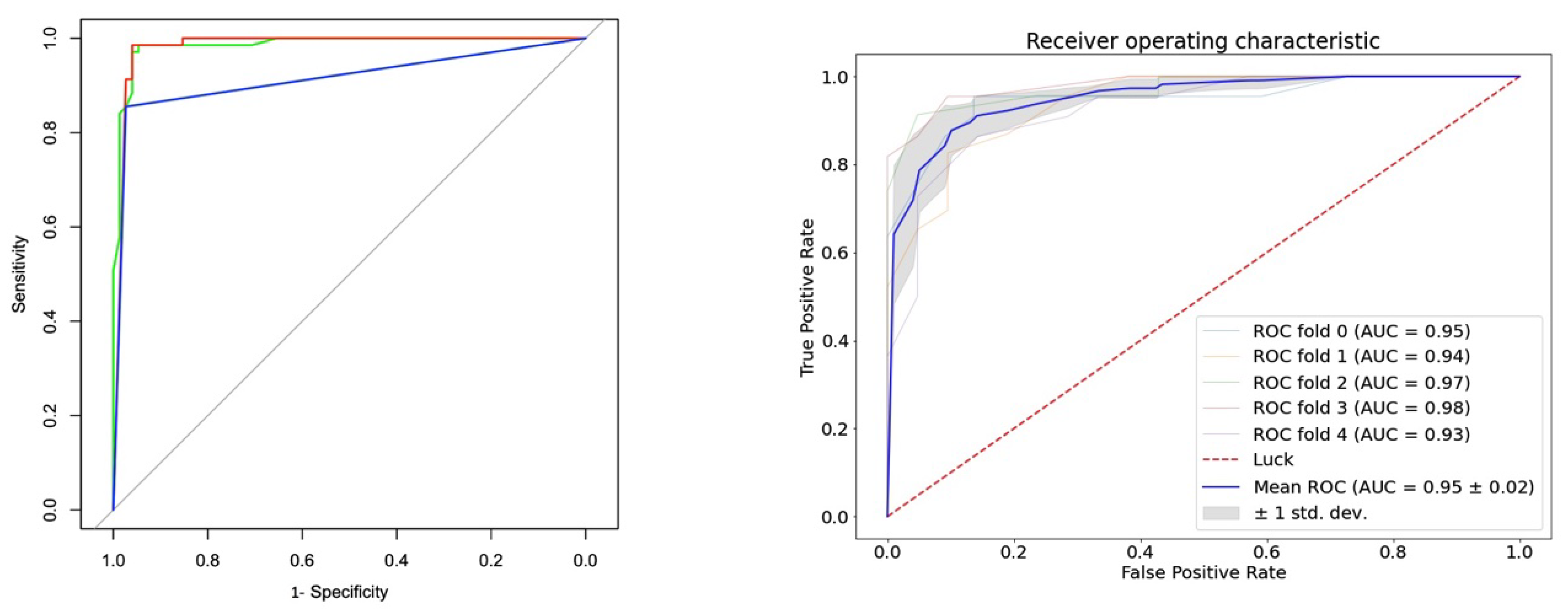
An ROC curve is a graph that shows how a binary classifier system’s diagnostic capacity changes when its discriminating threshold is altered. The rate, which is deviant from the true positive or sensitivity, is on the y-axis, and the specificity, which is deviant from the false positive, is on the x-axis. ROC might be seen as a power plot that depends on a Type I error. The ROC curves were plotted for RF, NBC, k-NN, and logistic regression based on the most important predictors determined by PCA for comparing 1-specificity versus sensitivity.
The metric that effectively averages the diagnostic accuracy over the range of test results is summarized by the overall area under the ROC curve. As the diagnostic test accuracy improves, the value becomes closer to 1.0, which is the gold standard AUC (AUC = 1). Since the sensitivity and 1-specificity are calculated nonparametrically, the nonparametric approach produces a jagged curve. The sensitivity/specificity pair associated with each point on the ROC curve corresponds to a specific decision threshold.
From Figure 6, the ROC curve that goes through the upper left corner indicates a test that has perfect discrimination, i.e., there is no overlap between the two distributions, meaning 100% sensitivity and 100% specificity. From Figure 6, the AUC values under the ROC are almost 0.96, 0.95, and 0.94 for RF, NBC/logistic regression, and k-NN, respectively. All the following models had an AUC close to 1, thereby indicating a high level of separability. Paired t-test to evaluate the comparison between machine learning classifiers are given in Table 2 below. It shows each model is statistically different.
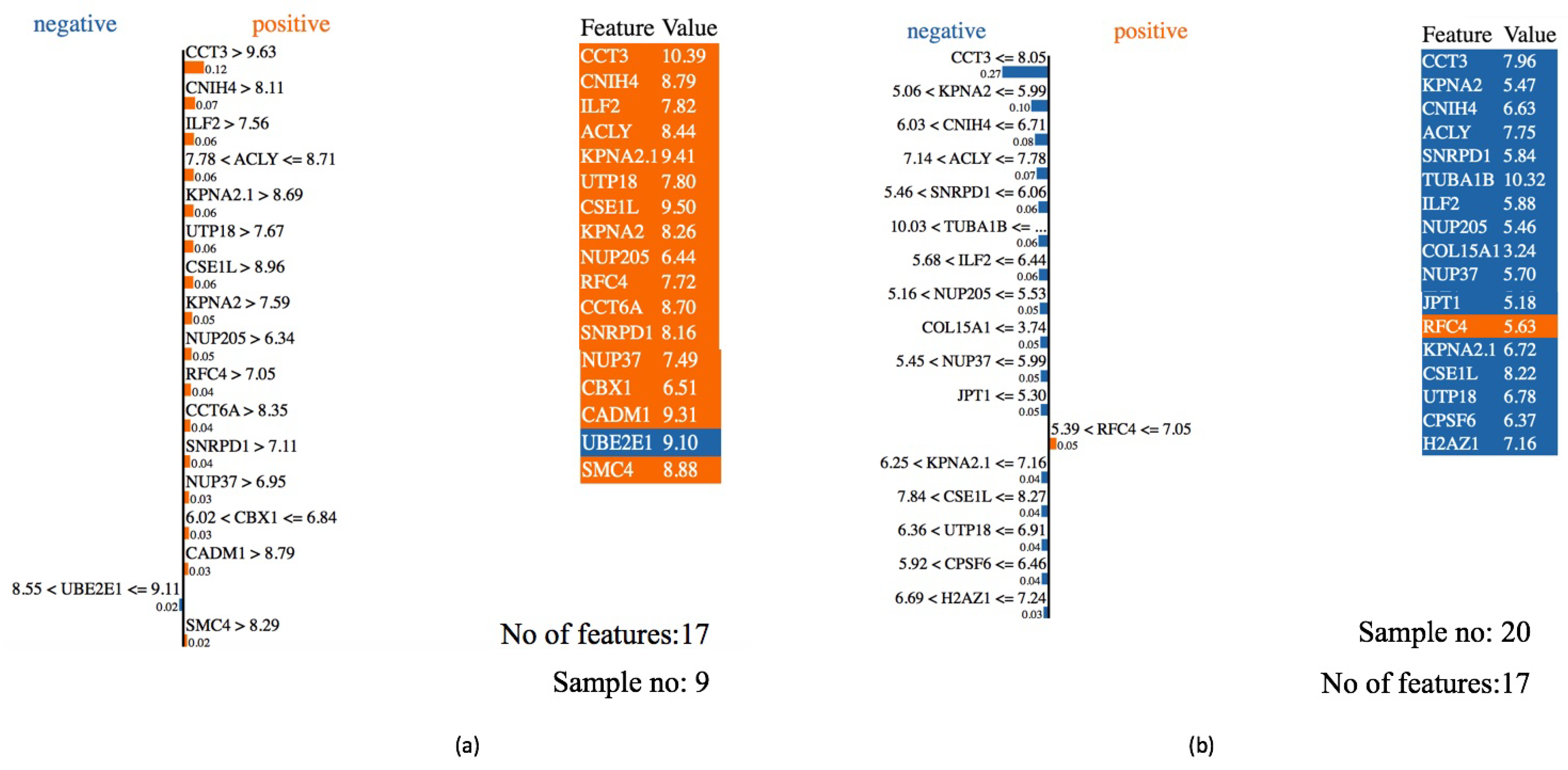
LIME was applied to determine the responsible features for HCC, and this gives us the order of importance of the features that either positively or negatively impact the response for each particular observation. Using variable importance ranking, the information for the top 17 genes was collected (see Appendix C). Pathway analysis was performed and is described in Appendix D. Figure 7 depicts two instances of a random forest model predicting that one patient has HCC while the other does not. An “explainer” then explains the prediction by emphasizing the features that are essential to the model.
LIME was used under an ML model with a relatively high accuracy score in this case. We selected two patients randomly from the dataset to apply LIME. The most significant 16 characteristics (genes) causing HCC in the two individuals are displayed in Figure 7. The model also classified the first person as a positive HCC patient with 98 % confidence, and the second person was classified as a negative HCC patient with 98 % confidence. Out of the top 16 most crucial features for the first patient, fifteen had positive effects on their response and two had a negative impact.
However, for the second patient, thirteen of them negatively impacted the response, and four of them positively impacted the response. It unambiguously shows that responsible genes can vary from patient to patient. Moreover, TUBA1B, CCT6A, ILF2, UTP18, CSE1L, CCT3, CNH4, ACLY, SMC4, CBX1, MCM6, RFC4, SNRPD1, TP53TG1, NUP205, and KPNA2 are the 16 important genes responsible for HCC, which are also confirmed by several authors in their articles.
KPNA2, and SMC4 showed up twice in the list of the top 18 genes. Therefore, only 16 gene names are listed above. TUBA1B expression was increased in HCC tumor tissues and proliferating HCC cells. In addition, poor overall survival and paclitaxel resistance in HCC patients is associated with increased TUBA1B expression [51]. CCT6A could stimulate HCC cell proliferation. As a prognostic biomarker for HCC, CCT6A could be considered as an oncogene of HCC [52].
ILF2 expression is associated with cell proliferation and apoptosis progression. ILF2 in HCC indicates that both in vitro and in vivo liver cancer cell proliferation are greatly affected by ILF2 [53]. UTP18 was obtained as one of the target genes in HCC [54]. Lasso–Cox regression analysis identified a four-gene prognostic model that incorporates clinical and gene expression data and has a positive effect. In addition, CSE1L was associated with survival time and status in HCC patients as determined by a univariate Cox regression analysis [55].
The comprehensive search for a clustered subset of genes comprises four genes upregulated in HCC and located in CCT3, demonstrating the significance of this gene in the expression analysis of HCC [56]. Time-dependent receiver operating characteristic (ROC), multivariable Cox regression analysis of clinical information, nomogram, and decision curve analysis (DCA) validated CNIH4 for more accurate prognosis prediction of HCC (DCA) [54]. ACLY, a novel gene with significance in metabolism and immune function and a prognostic gene panel in HCC are being studied.
It was suggested that inhibiting ACLY and immune checkpoints may shed light on HCC treatment [57]. CBX1 expression was significantly higher in HCC tissues compared with in non-tumor tissues [58]. Furthermore, CBX1 expression was associated with enormous tumor growth, poor tumor differentiation, and tumor vascular invasion [58]. MCM6 was found to be significantly upregulated in HCC tissues [59]. In HCC patients, increased MCM6 expression was associated with aggressive clinicopathological features and a worse prognosis [59].
These findings supported the findings from the Cancer Genome Atlas database (TCGA). Moreover, knocking down MCM6 significantly reduced HCC cell proliferation and migratory/invasive capability in vitro, as well as tumor volume, weight, and the number of pulmonary metastases in vivo. In addition, MCM6 promoted EMT and activated MEK/ERK signaling, according to mechanistic analyses [59]. More importantly, HCC patients had significantly higher serum MCM6 levels than did cirrhotic and healthy controls [59]. KPNA2 participates in cell differentiation, proliferation, apoptosis, immunological response, and viral infection to promote tumor growth and progression [60].
RFC4 is from the replication factor C (RFC) family [61], which is biologically active in various malignant liver tumors, and plays an important role in the proliferation, progression, invasion, and metastasis of cancer cells [62]. NUP205 is overexpressed in HCC tumors compared to neighboring normal tissues [63]. This gene may be associated with human HCC cell proliferation [63]. SNRPD1 was identified as part of a nine-gene signature associated with HCC prognosis [64].
High expression of this signature indicates a poor prognosis for HCC. In addition, increased levels of SNRPD1 are associated with HCC metastasis [64]. The overexpression of TP53TG1 enhanced HCC proliferation [65]. It was found that TP53TG1 has an oncogenic role in HCC, which gives a novel insight into the cell-type-specific function of TP53TG1 in HCC [65].
Overall, all the identified genes are significantly responsible for HCC and biologically connected to liver diseases. A hierarchical clustering tree is used to break down and summarize the association between the significant pathways identified in the enrichment. Since physicians now know which genes are responsible for HCC for a particular patient, it will help them to better treat the patient.
Moreover, we discuss some limitations and the future directions of this study. If random forest is not calibrated appropriately, it may overfit the data, which would cause it to perform well on training data but badly on test data. Large datasets may be constrained by the fact that, as the forest’s number of trees grows, so does the calculation time. Furthermore, LIME can be computationally expensive, especially for large datasets or complex models. The interpretation may not be representative of the entire dataset. LIME generates local explanations for specific instances, which may not represent the overall behavior of the model. The choice of hyperparameters in LIME can affect the interpretation of the model, and it may require tuning to obtain reliable results.
While random forest and LIME are effective methods overall, they have drawbacks and should only be used with care and a thorough grasp of both their advantages and disadvantages. PCA is a linear technique and may not capture complex interactions between the original features, which can limit its ability to model complex relationships in the data. Thus, in the future, instead of using PCA, one could use UMAP, t-SNE, or autoencoders. We recommend autoencoders. These are neural network models that learn to encode high-dimensional data into a lower-dimensional representation and then decode it back into the original space.
Moreover, instead of using LIME, one could use SHapley Additive exPlanations (SHAP), or anchors, which are a rule-based method for explaining the predictions of black-box models. Anchors generate human-readable and understandable rules that are interpretable and can be used to explain model predictions. Moreover, ML models rely on data to make predictions, and if the amount or quality of the data is limited, the accuracy of the model may be reduced.
In some cases, the data may be biased or incomplete, leading to errors in the predictions. In practice, AI and ML models are designed to optimize for accuracy while balancing other factors, such as the speed, efficiency, and interpretability. While 100% accuracy may not be achievable in all cases, the goal is to build models that are as accurate as possible given the constraints of the problem and the available data.

4. Conclusions

Our findings support prior research by demonstrating that machine-learning approaches may be used to discover responsible genes that have a substantial influence on HCC. According to Lee et al., precision medicine has shown that the genetic properties of cancer cells may be used to predict the treatment response, and new research suggests that gene–drug links may be predicted very precisely by investigating the cumulative impact of multiple genes at the same time [66]. By identifying the genes responsible for HCC using the RF model, we can develop novel treatments or improve existing therapies to prevent HCC in its early stages.
Due to the limited number of training instances, the availability of a large number of genes, and the various inherent uncertainties, microarray data analysis poses a challenge to conventional machine-learning approaches. One of the most important advantages of machine learning in the healthcare sector is its capacity to recognize and diagnose illnesses and ailments that would otherwise be challenging to diagnose. Due to the high dimensionality of the HCC microarray data, it is necessary to include feature selection to reduce the dimensionality of the data.
To reduce the dimensionality of the data, we used PCA for feature selection, selecting the 100 most essential genes to train the different machine-learning models. The accuracy of RF after feature selection using PCA was 96.54% and, before feature selection, was 87.41%. Based on the model’s classification accuracy, the random forest model was chosen as the final model, which fitted the LIME model as the explainable AI model based on the 16 top genes. The names of these genes are TUBA1B, CCT6A, ILF2, UTP18, CSE1L, CCT3, CNH4, ACLY, SMC4, CBX1, MCM6, RFC4, SNRPD1, TP53TG1, NUP205, and KPNA2.
The explainable AI addresses the challenges of understanding the model at the local level, allowing health professionals to choose whether or not the model should be adopted. When physicians recognize the most critical genes associated with HCC in a particular patient, they can treat that patient more effectively. The proposed framework may help clinicians to understand the gap between clinical and machine-intelligent reports based on an AI explanation. HCC is still associated with poor prognosis in patients with advanced disease [67].
This study shows how to improve HCC diagnosis in the early stages so that clinicians can obtain early information. AI or ML models are a modern technique for predicting diseases; however, these models are highly reliant on the available data; therefore, they cannot replace or challenge the current clinical practices, such as CT, MRI, biopsy, and other clinical techniques.

Author Contributions

Data Findings, M.E.H. and F.M.; Methodology, M.E.H., F.M. and M.S.H.; Writing: M.E.H., F.M., M.S.H. and J.L. All authors have read and agreed to the published version of the manuscript.

Funding

This research received no external funding.

Institutional Review Board Statement

This study considered a published dataset that is publicly available at the https://www.ncbi.nlm.nih.gov [30] accessed on 3 December 2021 use of the dataset for research purposes and scientific developments.

Informed Consent Statement

This research was conducted on human subject data. Data were obtained from open sources. The NIH received consent. For more details, visit the website [30].

Data Availability Statement

Data are available online at the https://www.ncbi.nlm.nih.gov/geo/query (accessed on 1 March 2021).

Acknowledgments

The authors are grateful to the unknown reviewers who helped to improve the quality of the paper.

Conflicts of Interest

The authors declare no conflict of interest.

Appendix A. Used Python and R Packages

Appendix A.1

The name of the package is Linear Models for Microarray and RNA-seq Data (LIMMA). Bioconductor version: Release (3.15) [31]. Use: Data analysis, linear models, and differential expression for microarray data.

Appendix A.2

Names of the Python packages: numpy, pandas, mlxtend.plotting, sklearn.model _selection, classifications models, etc.

Appendix B. Hyper-Parameters in the ML Models

  • Method: RF
Hyperparameter: n estimators: int, default = 100, criterion: gini, max depth: default = None, min samples split: default = 2, max features = ‘auto’, max leaf nodes = None, min impurity decrease = 0.0, min impurity split = None, bootstrap = True, oob score = False, n jobs = −1, random state = 0, verbose = 0, warm start = False, and class weight = ’balanced’.
  • Method: NBC
Hyperparameter: Priors: array-like of shape (n classes = 2). The class proportions for the training set used var smoothing: float, 1e-9; class prior: array of shape (n classes = 2), and the probability of each class.
var: ndarray of shape (n classes = 2, and n features = 100). Variance of each feature per class.
Method: Logistic Regression
Hyperparameter: Penalty: none. Tol: float. 1 e 4 . The other parameters are the default.
  • Method: k-NN
Hyperparameter: n neighbors: k = 3. The other parameters are the default.
Algorithm A1: The algorithm for the proposed framework.
Input: HCC dataset. Output: Final trained and tested model.
Step 1: Initialize the dataset.
- Load the HCC dataset.
Step 2: Preprocess the full dataset.
- Remove missing data and duplicates and normalize the dataset.
Step 3: Feature selection of the HCC dataset.
- Perform PCA to select the top 100 genes.
Step 4: Divide the dataset into two sets:
i. Training Set (66.67% of the dataset).
ii. Test Set (33.37% of the dataset).
- Randomly split the dataset into training and test sets.
Step 5: Train the models with the Training Set.
- Train multiple machine-learning models, such as random forest, SVM, logistic regression, and NBC using the 16 top genes by variable importance ranking.
Step 6: Test the trained models with the Test Set.
- Evaluate the performance of the trained models on the test set.
Step 7: Generate the confusion matrix and ROC analysis.
- Calculate the confusion matrix, ROC curve, and confidence interval.
Step 8: Generate the final trained and tested model.
- Select the best-performing model based on evaluation metrics.
Step 9: Send the final model to Explainable AI.
- Use the LIME algorithm to generate the top 16 genes that contribute to the final model’s decision.

Appendix C. HCC Gene Mining

The top 100 genes using PCA are presented below. Genes are listed here with Column ID notations. Based on the Gini index, the 17 top responsible genes are indicated in blue.
AFFYMETRIX
3PRIME IVT ID
NameSpeciesColumn ID
210987_x_attropomyosin 1 (TPM1)Homo sapiensV10434
210986_s_attropomyosin 1 (TPM1)Homo sapiensV10433
220917_s_atWD repeat domain 19 (WDR19)Homo sapiensV20281
221223_x_atcytokine-inducible SH2 containing protein (CISH)Homo sapiensV20586
215605_atnuclear receptor coactivator 2 (NCOA2)Homo sapiensV14978
204718_atEPH receptor B6 (EPHB6)Homo sapiensV4245
219828_atRAB, member RAS oncogene family like 6 (RABL6)Homo sapiensV19192
211072_x_attubulin alpha 1b (TUBA1B)Homo sapiensV10516
204690_atsyntaxin 8 (STX8)Homo sapiensV4217
201327_s_atchaperonin containing TCP1 subunit 6A (CCT6A)Homo sapiensV855
200750_s_atRAN, member RAS oncogene family (RAN)Homo sapiensV278
218421_atceramide kinase (CERK)Homo sapiensV17786
213455_atfamily with sequence similarity 114 member A1 (FAM114A1)Homo sapiensV12836
202146_atinterferon related developmental regulator 1 (IFRD1)Homo sapiensV1674
221351_at5-hydroxytryptamine receptor 1A (HTR1A)Homo sapiensV20714
200052_s_atinterleukin enhancer binding factor 2 (ILF2)Homo sapiensV73
214037_s_atcoiled-coil domain containing 22 (CCDC22)Homo sapiensV13416
203721_s_atUTP18 small subunit processome component (UTP18)Homo sapiensV3248.
221760_atmannosidase alpha class 1A member 1 (MAN1A1)Homo sapiensV21120
209030_s_atcell adhesion molecule 1 (CADM1)Homo sapiensV8524
212168_atRNA-binding motif protein 12 (RBM12)Homo sapiensV11554
203477_atcollagen type XV alpha 1 chain (COL15A1)Homo sapiensV3004
201112_s_atchromosome segregation 1 like (CSE1L)Homo sapiensV640
212519_atubiquitin conjugating enzyme E2 E1 (UBE2E1)Homo sapiensV11904
217889_s_atcytochrome b reductase 1 (CYBRD1)Homo sapiensV17254
202291_s_atmatrix Gla protein (MGP)Homo sapiensV1819
221664_s_atF11 receptor (F11R)Homo sapiensV21025
216867_s_atplatelet derived growth factor subunit A (PDGFA)Homo sapiensV16237
205463_s_atplatelet derived growth factor subunit A (PDGFA)Homo sapiensV4990
200612_s_atadaptor related protein complex 2 subunit beta 1 (AP2B1)Homo sapiensV140
200910_atchaperonin containing TCP1 subunit 3 (CCT3)Homo sapiensV438
210385_s_atendoplasmic reticulum aminopeptidase 1 (ERAP1)Homo sapiensV9863
218010_x_atpancreatic progenitor cell differentiation and proliferation factor (PPDPF)Homo sapiensV17375
218728_s_atcornichon family AMPA receptor auxiliary protein 4 (CNIH4)Homo sapiensV18092
209071_s_atregulator of G protein signaling 5 (RGS5)Homo sapiensV8565
218353_atregulator of G protein signaling 5 (RGS5)Homo sapiensV17718
202011_attight junction protein 1 (TJP1)Homo sapiensV1539
201873_s_atATP-binding cassette subfamily E member 1 (ABCE1)Homo sapiensV1401
209373_atmal, T cell differentiation protein like (MALL)Homo sapiensV8866
202469_s_atcleavage and polyadenylation specific factor 6 (CPSF6)Homo sapiensV1997
212473_s_atmicrotubule associated monooxygenase, calponin and LIM domain containing 2 (MICAL2)Homo sapiensV11858
218622_atnucleoporin 37 (NUP37)Homo sapiensV17987
201128_s_atATP citrate lyase (ACLY)Homo sapiensV656
201909_atribosomal protein S4 Y-linked 1 (RPS4Y1)Homo sapiensV1437
55872_aturidine-cytidine kinase 1 like 1 (UCKL1)Homo sapiensV22108
204020_atpurine rich element binding protein A (PURA)Homo sapiensV3547
202565_s_atsupervillin (SVIL)Homo sapiensV2093
208683_atcalpain 2 (CAPN2)Homo sapiensV8178
211974_x_atrecombination signal binding protein for immunoglobulin kappa J region (RBPJ)Homo sapiensV11361
203021_atsecretory leukocyte peptidase inhibitor (SLPI)Homo sapiensV2550
213139_atsnail family transcriptional repressor 2 (SNAI2)Homo sapiensV12522
218531_attransmembrane protein 134 (TMEM134)Homo sapiensV17896
201663_s_atstructural maintenance of chromosomes 4 (SMC4)Homo sapiensV1191
201664_atstructural maintenance of chromosomes 4 (SMC4)Homo sapiensV1192
211833_s_atBCL2 associated X, apoptosis regulator (BAX)Homo sapiensV11229
201177_s_atubiquitin-like modifier activating enzyme 2 (UBA2)Homo sapiensV705
200985_s_atCD59 molecule (CD59 blood group) (CD59)Homo sapiensV513
212463_atCD59 molecule (CD59 blood group) (CD59)Homo sapiensV11848
213911_s_atH2A.Z variant histone 1 (H2AZ1)Homo sapiensV13290
200853_atH2A.Z variant histone 1 (H2AZ1)Homo sapiensV381
201518_atchromobox 1 (CBX1)Homo sapiensV1046
202543_s_atglia maturation factor beta (GMFB)Homo sapiensV2071
204347_atadenylate kinase 4 (AK4)Homo sapiensV3874
205968_atpotassium voltage-gated channel modifier subfamily S member 3 (KCNS3)Homo sapiensV5495
219215_s_atsolute carrier family 39 member 4 (SLC39A4)Homo sapiensV18579
201930_atminichromosome maintenance complex component 6 (MCM6)Homo sapiensV1458
203041_s_atlysosomal associated membrane protein 2 (LAMP2)Homo sapiensV2570
202597_atinterferon regulatory factor 6 (IRF6)Homo sapiensV2125
212766_s_atinterferon stimulated exonuclease gene 20 like 2 (ISG20L2)Homo sapiensV12151
217755_atJupiter microtubule associated homolog 1 (JPT1)Homo sapiensV17120
208789_atcaveolae associated protein 1 (CAVIN1)Homo sapiensV8284
205361_s_atprefoldin subunit 4 (PFDN4)Homo sapiensV4888
200795_atSPARC-like 1 (SPARCL1)Homo sapiensV323
201181_atG protein subunit alpha i3 (GNAI3)Homo sapiensV709
212371_atdesumoylating isopeptidase 2 (DESI2)Homo sapiensV11756
203953_s_atclaudin 3 (CLDN3)Homo sapiensV3480
202790_atclaudin 7 (CLDN7)Homo sapiensV2318
204440_atCD83 molecule (CD83)Homo sapiensV3967
221578_atRas association domain family member 4 (RASSF4)Homo sapiensV20940
204023_atreplication factor C subunit 4 (RFC4)Homo sapiensV3550
213882_atTM2 domain containing 1 (TM2D1)Homo sapiensV13262
201200_atcellular repressor of E1A stimulated genes 1 (CREG1)Homo sapiensV728
213506_atF2R-like trypsin receptor 1 (F2RL1)Homo sapiensV12887
218418_s_atKN motif and ankyrin repeat domains 2 (KANK2)Homo sapiensV17783
204106_attestis associated actin remodelling kinase 1 (TESK1)Homo sapiensV3633
202690_s_atsmall nuclear ribonucleoprotein D1 polypeptide (SNRPD1)Homo sapiensV2218
208541_x_attranscription factor A, mitochondrial (TFAM)Homo sapiensV8039
211754_s_atsolute carrier family 25 member 17 (SLC25A17)Homo sapiensV11154
207996_s_atlow density lipoprotein receptor class A domain containing 4 (LDLRAD4)Homo sapiensV7507
213242_x_atcentrosomal protein 170B (CEP170B)Homo sapiensV12624
202072_atheterogeneous nuclear ribonucleoprotein L (HNRNPL)Homo sapiensV1600
205542_atSTEAP family member 1 (STEAP1)Homo sapiensV5069.
220264_s_atG protein-coupled receptor 107 (GPR107)Homo sapiensV19628
209917_s_atTP53 target 1 (TP53TG1)Homo sapiensV9403
210740_s_atinositol-tetrakisphosphate 1-kinase (ITPK1)Homo sapiensV10201
212043_attrans-golgi network protein 2 (TGOLN2)Homo sapiensV11429
212247_atnucleoporin 205 (NUP205)Homo sapiensV11633
211762_s_atkaryopherin subunit alpha 2 (KPNA2)Homo sapiensV11161
201088_atkaryopherin subunit alpha 2 (KPNA2)Homo sapiensV616
222344_atInformation Unknown V21703

Appendix D. Pathway Analysis

A controlled vocabulary is provided by gene ontology (GO) analysis, which may be used to characterize the properties of genes and gene products in any organism. In order to determine the molecular functions of differentially expressed genes, we conducted our analysis using ShinyGO 0.76 (http://bioinformatics.sdstate.edu/go/) (accessed on 12 November 2022).
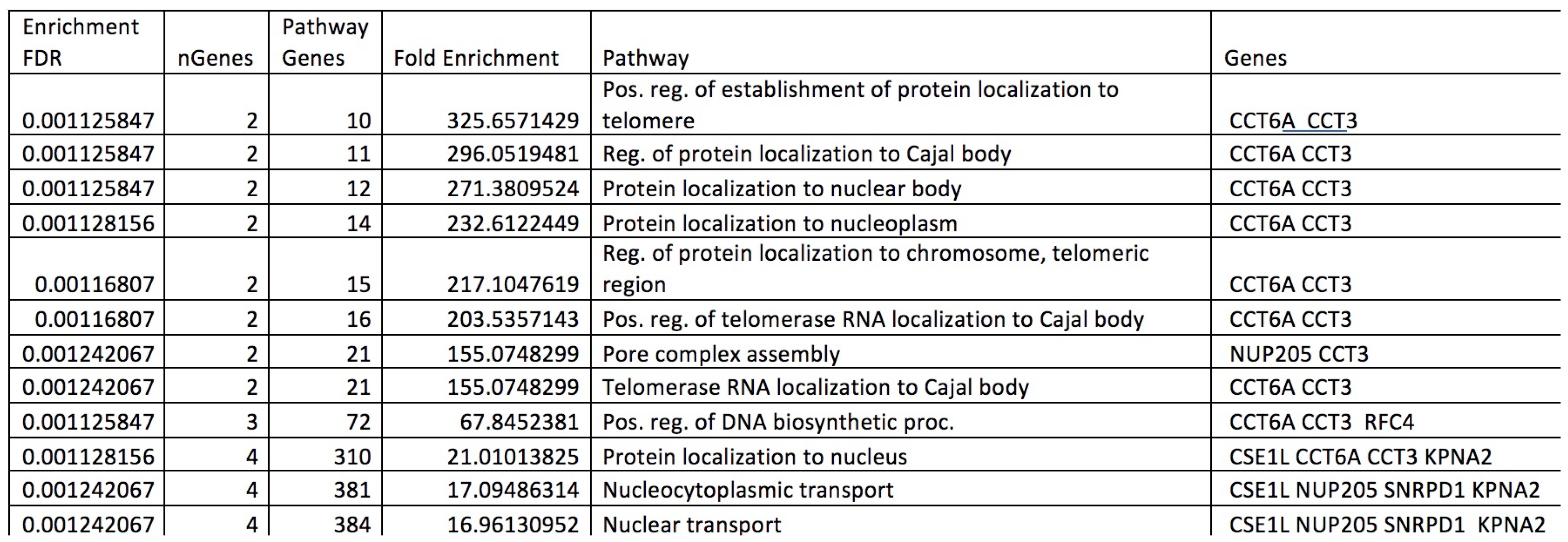
ShinyGO 0.76 is a collection of tools for integrating and visualizing data based on pathways. It visualizes and maps user data on appropriate route graphs. We use Figure A1, Figure A2, Figure A3 and Figure A4 to describe the pathway analysis of the HCC data.
Network interpretation: This interactive map also demonstrates the connection between several enriched pathways. If two nodes share at least 20% of their genes, then they are linked. Darker nodes indicate more highly enriched gene sets. Larger nodes reflect larger gene sets. More genes have overlapping regions if the margin is thicker.
Tree interpretation: The association between the significant pathways identified in the Enrichment is broken down and summarized using a hierarchical clustering tree. The pathways that share a large number of genes are grouped together. Larger dots represent more significant p-values. Adjusting the width of your browser window will result in a corresponding change to the width of the plot.
Figure A1. Bar plot indicates the fold enrichment versus pathways.
Appliedmath 03 00022 g0a1
Figure A2. Integrating and visualizing the top 17 genes based on pathways.
Appliedmath 03 00022 g0a2
Figure A3. Dendogram that shows the pathway hierarchical clustering.
Appliedmath 03 00022 g0a3
Figure A4. Gene set enrichment score.
Appliedmath 03 00022 g0a4

References

  1. El-Serag, H.B.; Kanwal, F. Epidemiology of hepatocellular carcinoma in the United States: Where are we? Where do we go? Hepatology 2014, 60, 1767. [Google Scholar] [CrossRef] [PubMed]
  2. Guan, X. Cancer metastases: Challenges and opportunities. Acta Pharm. Sin. B 2015, 5, 402–418. [Google Scholar] [CrossRef] [PubMed]
  3. Roessler, S.; Jia, H.L.; Budhu, A.; Forgues, M.; Ye, Q.H.; Lee, J.S.; Thorgeirsson, S.S.; Sun, Z.; Tang, Z.Y.; Qin, L.X.; et al. A unique metastasis gene signature enables prediction of tumor relapse in early-stage hepatocellular carcinoma patients. Cancer Res. 2010, 70, 10202–10212. [Google Scholar] [CrossRef] [PubMed]
  4. Roessler, S.; Long, E.L.; Budhu, A.; Chen, Y.; Zhao, X.; Ji, J.; Walker, R.; Jia, H.L.; Ye, Q.H.; Qin, L.X.; et al. Integrative genomic identification of genes on 8p associated with hepatocellular carcinoma progression and patient survival. Gastroenterology 2012, 142, 957–966. [Google Scholar] [CrossRef]
  5. Zhao, X.; Parpart, S.; Takai, A.; Roessler, S.; Budhu, A.; Yu, Z.; Blank, M.; Zhang, Y.E.; Jia, H.L.; Ye, Q.H.; et al. Integrative genomics identifies YY1AP1 as an oncogenic driver in EpCAM+ AFP+ hepatocellular carcinoma. Oncogene 2015, 34, 5095–5104. [Google Scholar] [CrossRef]
  6. Wang, Y.; Gao, B.; Tan, P.Y.; Handoko, Y.A.; Sekar, K.; Deivasigamani, A.; Seshachalam, V.P.; Ouyang, H.Y.; Shi, M.; Xie, C.; et al. Genome-wide CRISPR knockout screens identify NCAPG as an essential oncogene for hepatocellular carcinoma tumor growth. FASEB J. 2019, 33, 8759–8770. [Google Scholar] [CrossRef]
  7. Lu, Y.; Xu, W.; Ji, J.; Feng, D.; Sourbier, C.; Yang, Y.; Qu, J.; Zeng, Z.; Wang, C.; Chang, X.; et al. Alternative splicing of the cell fate determinant Numb in hepatocellular carcinoma. Hepatology 2015, 62, 1122–1131. [Google Scholar] [CrossRef]
  8. Chen, S.; Fang, H.; Li, J.; Shi, J.; Zhang, J.; Wen, P.; Wang, Z.; Yang, H.; Cao, S.; Zhang, H.; et al. Microarray analysis for expression profiles of lncRNAs and circRNAs in rat liver after brain-dead donor liver transplantation. BioMed Res. Int. 2019, 2019, 5604843. [Google Scholar] [CrossRef]
  9. Chen, S.L.; Zhu, Z.X.; Yang, X.; Liu, L.L.; He, Y.F.; Yang, M.M.; Guan, X.Y.; Wang, X.; Yun, J.P. Cleavage and polyadenylation specific factor 1 promotes tumor progression via alternative polyadenylation and splicing in hepatocellular carcinoma. Front. Cell Dev. Biol. 2021, 9, 616835. [Google Scholar] [CrossRef]
  10. Ashburner, M.; Ball, C.A.; Blake, J.A.; Botstein, D.; Butler, H.; Cherry, J.M.; Davis, A.P.; Dolinski, K.; Dwight, S.S.; Eppig, J.T.; et al. Gene ontology: Tool for the unification of biology. Nat. Genet. 2000, 25, 25–29. [Google Scholar] [CrossRef]
  11. García-Campos, M.A.; Espinal-Enríquez, J.; Hernández-Lemus, E. Pathway analysis: State of the art. Front. Physiol. 2015, 6, 383. [Google Scholar] [CrossRef]
  12. Folger, O.; Jerby, L.; Frezza, C.; Gottlieb, E.; Ruppin, E.; Shlomi, T. Predicting selective drug targets in cancer through metabolic networks. Mol. Syst. Biol. 2011, 7, 501. [Google Scholar] [CrossRef]
  13. Hansen, M.; Dubayah, R.; DeFries, R. Classification trees: An alternative to traditional land cover classifiers. Int. J. Remote Sens. 1996, 17, 1075–1081. [Google Scholar] [CrossRef]
  14. Huang, C.; Davis, L.; Townshend, J. An assessment of support vector machines for land cover classification. Int. J. Remote Sens. 2002, 23, 725–749. [Google Scholar] [CrossRef]
  15. Rogan, J.; Miller, J.A.; Stow, D.A.; Franklin, J.; Levien, L.M.; Fischer, C. Land-Cover Change Monitoring with Classification Trees Using Landsat TM and Ancillary Data. Photogramm. Eng. Remote. Sens. 2003, 69, 793–804. [Google Scholar] [CrossRef]
  16. Foody, G.M. Land cover classification by an artificial neural network with ancillary information. Int. J. Geogr. Inf. Syst. 1995, 9, 527–542. [Google Scholar] [CrossRef]
  17. Friedl, M.A.; Brodley, C.E. Decision tree classification of land cover from remotely sensed data. Remote Sens. Environ. 1997, 61, 399–409. [Google Scholar] [CrossRef]
  18. Breiman, L. Randomizing outputs to increase prediction accuracy. Mach. Learn. 2000, 40, 229–242. [Google Scholar] [CrossRef]
  19. Kleinberg, E.M. On the algorithmic implementation of stochastic discrimination. IEEE Trans. Pattern Anal. Mach. Intell. 2000, 22, 473–490. [Google Scholar] [CrossRef]
  20. Santos, M.S.; Abreu, P.H.; García-Laencina, P.J.; Simão, A.; Carvalho, A. A new cluster-based oversampling method for improving survival prediction of hepatocellular carcinoma patients. J. Biomed. Inform. 2015, 58, 49–59. [Google Scholar] [CrossRef]
  21. Acharya, U.R.; Faust, O.; Molinari, F.; Sree, S.V.; Junnarkar, S.P.; Sudarshan, V. Ultrasound-based tissue characterization and classification of fatty liver disease: A screening and diagnostic paradigm. Knowl.-Based Syst. 2015, 75, 66–77. [Google Scholar] [CrossRef]
  22. Muflikhah, L.; Widodo, N.; Mahmudy, W.F.; Solimun; Wahibah, N.N. Detection of Hepatoma based on Gene Expression using Unitary Matrix of Singular Vector Decomposition. Int. J. Adv. Comput. Sci. Appl. 2021, 12, 8. [Google Scholar] [CrossRef]
  23. Książek, W.; Hammad, M.; Pławiak, P.; Acharya, U.R.; Tadeusiewicz, R. Development of novel ensemble model using stacking learning and evolutionary computation techniques for automated hepatocellular carcinoma detection. Biocybern. Biomed. Eng. 2020, 40, 1512–1524. [Google Scholar] [CrossRef]
  24. Zhang, H. The optimality of naive Bayes. Aa 2004, 1, 3. [Google Scholar]
  25. Caruana, R.; Niculescu-Mizil, A. An empirical comparison of supervised learning algorithms. In Proceedings of the 23rd International Conference on Machine Learning, Virtual, 26–28 August 2006; pp. 161–168. [Google Scholar]
  26. Ribeiro, M.T.; Singh, S.; Guestrin, C. “Why should i trust you?” Explaining the predictions of any classifier. In Proceedings of the 22nd ACM SIGKDD International Conference on Knowledge Discovery and Data Mining, San Francisco, CA, USA, 13–17 August 2016; pp. 1135–1144. [Google Scholar]
  27. Palatnik de Sousa, I.; Maria Bernardes Rebuzzi Vellasco, M.; Costa da Silva, E. Local interpretable model-agnostic explanations for classification of lymph node metastases. Sensors 2019, 19, 2969. [Google Scholar] [CrossRef]
  28. Kumarakulasinghe, N.B.; Blomberg, T.; Liu, J.; Leao, A.S.; Papapetrou, P. Evaluating local interpretable model-agnostic explanations on clinical machine learning classification models. In Proceedings of the 2020 IEEE 33rd International Symposium on Computer-Based Medical Systems (CBMS), Rochester, MN, USA, 28–30 July 2020; pp. 7–12. [Google Scholar]
  29. Davagdorj, K.; Li, M.; Ryu, K.H. Local interpretable model-agnostic explanations of predictive models for hypertension. In Advances in Intelligent Information Hiding and Multimedia Signal Processing; Springer: Berlin/Heidelberg, Germany, 2021; pp. 426–433. [Google Scholar]
  30. W3Techs. Geo Accession Viewer. 2010. Available online: https://www.ncbi.nlm.nih.gov/geo/query/acc.cgi (accessed on 1 November 2022).
  31. Reinhardt, J.; Landsberg, J.; Schmid-Burgk, J.L.; Ramis, B.B.; Bald, T.; Glodde, N.; Lopez-Ramos, D.; Young, A.; Ngiow, S.F.; Nettersheim, D.; et al. MAPK signaling and inflammation link melanoma phenotype switching to induction of CD73 during immunotherapy. Cancer Res. 2017, 77, 4697–4709. [Google Scholar] [CrossRef]
  32. Abdi, H.; Williams, L.J. Principal component analysis. Wiley Interdiscip. Rev. Comput. Stat. 2010, 2, 433–459. [Google Scholar] [CrossRef]
  33. Watson, D.S. Interpretable machine learning for genomics. Hum. Genet. 2021, 141, 1499–1513. [Google Scholar] [CrossRef]
  34. Strobl, C.; Boulesteix, A.L.; Kneib, T.; Augustin, T.; Zeileis, A. Conditional variable importance for random forests. BMC Bioinform. 2008, 9, 307. [Google Scholar] [CrossRef]
  35. Raileanu, L.E.; Stoffel, K. Theoretical comparison between the gini index and information gain criteria. Ann. Math. Artif. Intell. 2004, 41, 77–93. [Google Scholar] [CrossRef]
  36. Tangirala, S. Evaluating the impact of GINI index and information gain on classification using decision tree classifier algorithm. Int. J. Adv. Comput. Sci. Appl. 2020, 11, 612–619. [Google Scholar] [CrossRef]
  37. Leung, K.M. Naive bayesian classifier. Polytechnic University Department of Computer Science/Finance and Risk Engineering. 2007, 2007, 123–156. Available online: https://cse.engineering.nyu.edu/~mleung/FRE7851/f07/naiveBayesianClassifier.pdf (accessed on 2 October 2022).
  38. Langarizadeh, M.; Moghbeli, F. Applying naive bayesian networks to disease prediction: A systematic review. Acta Inform. Medica 2016, 24, 364. [Google Scholar] [CrossRef]
  39. Komarek, P. Logistic Regression for Data Mining and High-Dimensional Classification; Carnegie Mellon University: Pittsburgh, PA, USA, 2004. [Google Scholar]
  40. Mucherino, A.; Papajorgji, P.J.; Pardalos, P.M. K-nearest neighbor classification. In Data Mining in Agriculture; Springer: Berlin/Heidelberg, Germany, 2009; pp. 83–106. [Google Scholar]
  41. Laaksonen, J.; Oja, E. Classification with learning k-nearest neighbors. In Proceedings of the International Conference on Neural Networks (ICNN’96), Washington, DC, USA, 3–6 June 1996; Volume 3, pp. 1480–1483. [Google Scholar]
  42. Jiang, L.; Cai, Z.; Wang, D.; Jiang, S. Survey of improving k-nearest-neighbor for classification. In Proceedings of the Fourth International Conference on Fuzzy Systems and Knowledge Discovery (FSKD 2007), Haikou, China, 24–27 August 2007; Volume 1, pp. 679–683. [Google Scholar]
  43. Zhang, C.; Ma, Y. Ensemble Machine Learning: Methods and Applications; Springer: Berlin/Heidelberg, Germany, 2012. [Google Scholar]
  44. Wu, M.; Liu, Z.; Zhang, A.; Li, N. Identification of key genes and pathways in hepatocellular carcinoma: A preliminary bioinformatics analysis. Medicine 2019, 98, e14287. [Google Scholar] [CrossRef]
  45. Raschka, S. Model evaluation, model selection, and algorithm selection in machine learning. arXiv 2018, arXiv:1811.12808. [Google Scholar]
  46. Pratt, J.W. Remarks on zeros and ties in the Wilcoxon signed rank procedures. J. Am. Stat. Assoc. 1959, 54, 655–667. [Google Scholar] [CrossRef]
  47. Wilcoxon, F. Individual comparisons by ranking methods. In Breakthroughs in Statistics; Springer: Berlin/Heidelberg, Germany, 1992; pp. 196–202. [Google Scholar]
  48. Fawcett, T. An introduction to ROC analysis. Pattern Recognit. Lett. 2006, 27, 861–874. [Google Scholar] [CrossRef]
  49. Zou, K.H.; O’Malley, A.J.; Mauri, L. Receiver-operating characteristic analysis for evaluating diagnostic tests and predictive models. Circulation 2007, 115, 654–657. [Google Scholar] [CrossRef]
  50. Taherdoost, H. Sampling methods in research methodology; how to choose a sampling technique for research; How to choose a sampling technique for research. Int. J. Acad. Res. Manag. 2016, 5, 18–27. [Google Scholar]
  51. Lu, C.; Zhang, J.; He, S.; Wan, C.; Shan, A.; Wang, Y.; Yu, L.; Liu, G.; Chen, K.; Shi, J.; et al. Increased α-tubulin1b expression indicates poor prognosis and resistance to chemotherapy in hepatocellular carcinoma. Dig. Dis. Sci. 2013, 58, 2713–2720. [Google Scholar] [CrossRef]
  52. Zeng, G.; Wang, J.; Huang, Y.; Lian, Y.; Chen, D.; Wei, H.; Lin, C.; Huang, Y. Overexpressing CCT6A contributes to cancer cell growth by affecting the G1-To-S phase transition and predicts a negative prognosis in hepatocellular carcinoma. OncoTargets Ther. 2019, 12, 10427. [Google Scholar] [CrossRef] [PubMed]
  53. Cheng, S.; Jiang, X.; Ding, C.; Du, C.; Owusu-Ansah, K.G.; Weng, X.; Hu, W.; Peng, C.; Lv, Z.; Tong, R.; et al. Expression and critical role of interleukin enhancer binding factor 2 in hepatocellular carcinoma. Int. J. Mol. Sci. 2016, 17, 1373. [Google Scholar] [CrossRef]
  54. Wang, Z.; Pan, L.; Guo, D.; Luo, X.; Tang, J.; Yang, W.; Zhang, Y.; Luo, A.; Gu, Y.; Pan, Y. A novel five-gene signature predicts overall survival of patients with hepatocellular carcinoma. Cancer Med. 2021, 10, 3808–3821. [Google Scholar] [CrossRef] [PubMed]
  55. Yan, J.; Cao, J.; Chen, Z. Mining prognostic markers of Asian hepatocellular carcinoma patients based on the apoptosis-related genes. BMC Cancer 2021, 21, 175. [Google Scholar] [CrossRef] [PubMed]
  56. Skawran, B.; Steinemann, D.; Weigmann, A.; Flemming, P.; Becker, T.; Flik, J.; Kreipe, H.; Schlegelberger, B.; Wilkens, L. Gene expression profiling in hepatocellular carcinoma: Upregulation of genes in amplified chromosome regions. Mod. Pathol. 2008, 21, 505–516. [Google Scholar] [CrossRef]
  57. Xu, Y.; Zhang, Z.; Xu, D.; Yang, X.; Zhou, L.; Zhu, Y. Identification and integrative analysis of ACLY and related gene panels associated with immune microenvironment reveal prognostic significance in hepatocellular carcinoma. Cancer Cell Int. 2021, 21, 1–20. [Google Scholar] [CrossRef]
  58. Yang, Y.F.; Pan, Y.H.; Tian, Q.H.; Wu, D.C.; Su, S.G. CBX1 indicates poor outcomes and exerts oncogenic activity in hepatocellular carcinoma. Transl. Oncol. 2018, 11, 1110–1118. [Google Scholar] [CrossRef]
  59. Liu, M.; Hu, Q.; Tu, M.; Wang, X.; Yang, Z.; Yang, G.; Luo, R. MCM6 promotes metastasis of hepatocellular carcinoma via MEK/ERK pathway and serves as a novel serum biomarker for early recurrence. J. Exp. Clin. Cancer Res. 2018, 37, 1–13. [Google Scholar] [CrossRef]
  60. Han, Y.; Wang, X. The emerging roles of KPNA2 in cancer. Life Sci. 2020, 241, 117140. [Google Scholar] [CrossRef]
  61. Li, Y.; Gan, S.; Ren, L.; Yuan, L.; Liu, J.; Wang, W.; Wang, X.; Zhang, Y.; Jiang, J.; Zhang, F.; et al. Multifaceted regulation and functions of replication factor C family in human cancers. Am. J. Cancer Res. 2018, 8, 1343. [Google Scholar]
  62. Lee, C.F.; Ling, Z.Q.; Zhao, T.; Fang, S.H.; Chang, W.C.; Lee, S.C.; Lee, K.R. Genomic-wide analysis of lymphatic metastasis-associated genes in human hepatocellular carcinoma. World J. Gastroenterol. WJG 2009, 15, 356. [Google Scholar] [CrossRef]
  63. Deng, Z.; Huang, K.; Liu, D.; Luo, N.; Liu, T.; Han, L.; Du, D.; Lian, D.; Zhong, Z.; Peng, J. Key Candidate Prognostic Biomarkers Correlated with Immune Infiltration in Hepatocellular Carcinoma. J. Hepatocell. Carcinoma 2021, 8, 1607. [Google Scholar] [CrossRef]
  64. Yao, X.; Lu, C.; Shen, J.; Jiang, W.; Qiu, Y.; Zeng, Y.; Li, L. A novel nine gene signature integrates stemness characteristics associated with prognosis in hepatocellular carcinoma. Biocell 2021, 45, 1425. [Google Scholar] [CrossRef]
  65. Lu, Q.; Guo, Q.; Xin, M.; Lim, C.; Gamero, A.M.; Gerhard, G.S.; Yang, L. LncRNA TP53TG1 Promotes the Growth and Migration of Hepatocellular Carcinoma Cells via Activation of ERK Signaling. Non-Coding RNA 2021, 7, 52. [Google Scholar] [CrossRef]
  66. Lee, B.K.B.; Tiong, K.H.; Chang, J.K.; Liew, C.S.; Abdul Rahman, Z.A.; Tan, A.C.; Khang, T.F.; Cheong, S.C. DeSigN: Connecting gene expression with therapeutics for drug repurposing and development. BMC Genom. 2017, 18, 934. [Google Scholar] [CrossRef]
  67. Trevisani, F.; Cantarini, M.; Wands, J.; Bernardi, M. Recent advances in the natural history of hepatocellular carcinoma. Carcinogenesis 2008, 29, 1299–1305. [Google Scholar] [CrossRef] [PubMed]
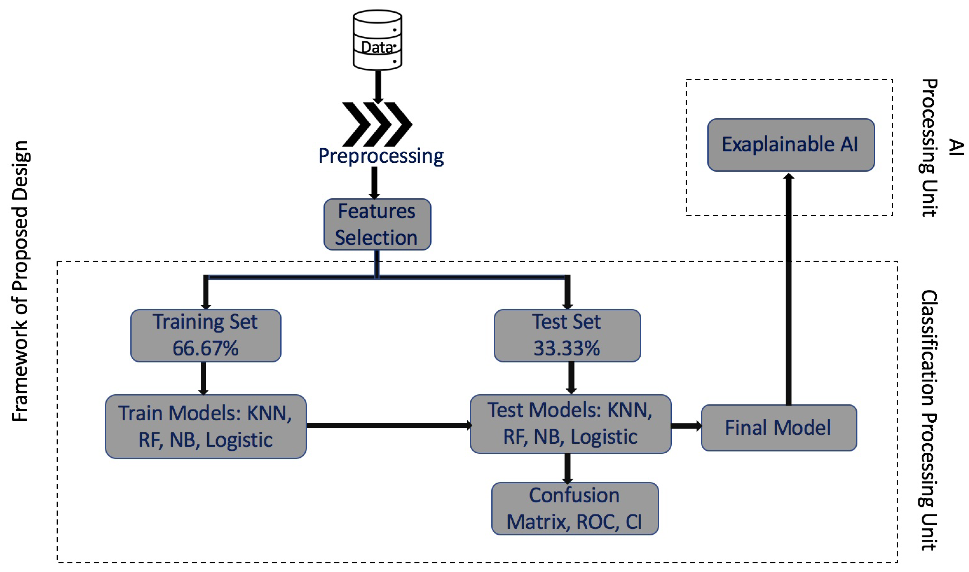
Figure 1. Diagram for ML/AI approach for microarray analysis of gene expression data. There are two main process steps: the first is a classification processing unit where training and test data are used to select the best model, and the second one is an AI processing unit for the global explanation.
Appliedmath 03 00022 g001
Figure 2. Heatmap of top 100 genes obtained from PCA. Due to lack of space, this plot represents only 25 gene names in the horizontal line. The names of the top 100 genes are presented in Appendix C.
Appliedmath 03 00022 g002
Figure 3. The left panel indicates errors for a growing number of trees in the random forest algorithm. For different values of the mtry parameter, the random forest error rates (calculated from out-of-bag situations) are shown as a function of the number of trees. This is based on the random forest voting method used to estimate gene expression response 1 in early testing. The right panel displays the top 17 variables (genes) based on variable importance rankings calculated from the Gini index. The mean decrease Gini is between 0 and 15. For example, CCT3 and KPNA2 show the highest values of the mean decrease Gini.
Appliedmath 03 00022 g003
Figure 4. Comparison of confusion matrices for four different classifiers. Position (0,0) is the true positive, and (1,1) is the true negative. Position (1,0) is the false positive, and (0,1) is the false negative.
Appliedmath 03 00022 g004
Figure 5. Plot that shows the comparison of the accuracy for four different classifiers measured in percentage. The names of the ML classifiers are given on the horizontal axis.
Appliedmath 03 00022 g005
Figure 6. The left panel shows the area under the ROC curves for different ML models. The green line indicates RF, the red line indicates NBC/logistic regression, and the blue line indicates k-NN classifiers for AUC under ROC curves. In the right panel, the five-fold cross-validation was used in order to collect multiple estimates and assess variability for the RF model.
Appliedmath 03 00022 g006
Figure 7. LIME outcomes for the RF classifier for HCC patients. Left panel (a) the credentials of sample 9 of the gene dataset. Right panel (b) the credentials of sample 20 of the gene dataset. The blue color suggests that the gene causes negative effects, and the orange color suggests that the gene causes positive effects on HCC.
Appliedmath 03 00022 g007
Table 1. Performancefor HCC gene expression data classifiers.
Methods Sensitivity Specificity Precision F 1 MCC σ 2
RF 0.9601 0.9710 0.9730 0.9664 0.9303 0.0335
NBC 0.9600 0.9565 0.9600 0.9600 0.9165 0.0390
Logistic Regression 0.9600 0.9565 0.9600 0.9600 0.9165 0.0391
k-NN 0.9263 0.9828 0.9888 0.9565 0.9117 0.0482
Table 2. Hypothesis testing for comparing classifiers.
Methods H 0 : RF & NBC Are Equivalent H 0 : RF & k-NN Are Equivalent H 0 : NBC & k-NN Are Equivalent
p-value 0.0157 0.0253 0.083
Disclaimer/Publisher’s Note: The statements, opinions and data contained in all publications are solely those of the individual author(s) and contributor(s) and not of MDPI and/or the editor(s). MDPI and/or the editor(s) disclaim responsibility for any injury to people or property resulting from any ideas, methods, instructions or products referred to in the content.