Abstract
A mathematical description of catastrophe in complex systems modeled as a network is presented with emphasis on network topology and its relationship to risk and resilience. We present mathematical formulas for computing risk, resilience, and likelihood of faults in nodes/links of network models of complex systems and illustrate the application of the formulas to simulation of catastrophic failure. This model is not related to nonlinear “Catastrophe theory” by René Thom, E.C. Zeeman and others. Instead, we present a strictly probabilistic network model for estimating risk and resilience—two useful metrics used in practice. We propose a mathematical model of exceedance probability, risk, and resilience and show that these properties depend wholly on vulnerability, consequence, and properties of the network representation of the complex system. We use simulation of the network under simulated stress causing one or more nodes/links to fail, to extract properties of risk and resilience. In this paper two types of stress are considered: viral cascades and flow cascades. One unified definition of risk, MPL, is proposed, and three kinds of resilience illustrated—viral cascading, blocking node/link, and flow resilience. The principal contributions of this work are new equations for risk and resilience and measures of resilience based on vulnerability of individual nodes/links and network topology expressed in terms of spectral radius, bushy, and branchy metrics. We apply the model to a variety of networks—hypothetical and real—and show that network topology needs to be included in any definition of network risk and resilience. In addition, we show how simulations can identify likely future faults due to viral and flow cascades. Simulations of this nature are useful to the practitioner.
1. Introduction
The primary goal of mathematics of catastrophe is to determine the likelihood, size a.k.a. consequence, and level of resistance to failure a.k.a. resilience, should a system partially or completely collapse. In the following, we develop three mathematical equations for likelihood, size, and resilience, and suggest mathematical means of predicting location of faults in complex systems represented as a network:
- Likelihood, EP(x): exceedance probability, and risk, (x)
- Maximum Probable Loss, MPL =
- Resilience, Z
- Cascading Fault prediction, cF
It is assumed that failure is instigated by some kind of stress to the system. Without stress, we assume the system continues to function properly and without fault. A fault occurs wherever a component of a system breaks down due to stress. Wear-and-tear is a kind of stress, so eventually all systems fail. Other kinds of stress explored here manifest in terms of faults propagating through a system of components due to contiguous linkages or induced by overloading and congesting non-contiguous components. These are called viral and flow stress, respectively, but other forms of stress are possible. Resilience is tolerance of stress and an essential property of systems that daily life depends on. We illustrate two forms of stress—viral cascades and overloading cascades in networks that support the flow of a commodity.
Since the occurrence of stress leading to one or more faults cannot be predicted, a mathematical treatment of catastrophe is necessarily stochastic. Hence, catastrophic modeling employs probability theory, but in an unusual and unique way. Instead of treating failures as samples taken from a probability density function, the mathematics of catastrophe model unpredictable failures as exceedance probabilities, i.e., the probability that a failure results in a consequence that equals or exceeds some threshold. This approach allows engineers and insurance companies to anticipate and prepare for the worst-case scenario rather than the average-case scenario.
Mathematical modeling of failures, disasters, catastrophes, and unexpected events has a long history, but there has been little progress in terms of rigorous foundations. Insurance companies have developed probability models based on the probability of events that exceed a certain cost, and stock market analysts have applied sophisticated statistical methods of computing risk, but these only partially constitute a mathematical foundation for catastrophic events. Here we present a comprehensive and rigorous mathematical foundation for catastrophic events emphasizing cause-and-effect propagation in complex systems. The math is based on the venerable power law and its application to risk and resilience.
Essentially, this foundation is a model based on representing complex systems prone to failure as networks with stochastic properties such as vulnerability and exceedance probability of failure and risk. The principal result is that a catastrophic event follows some kind of stress—a.k.a. threat—which can be quantified and depends partly on the topological structure of the system modeled as a network. Additionally, once we have a network model of a system, we can drill down to individual components—nodes and links—to determine the likelihood of an initial fault propagating throughout a network. This enables prediction of network failures in terms of probability of component failure.
Simulation is employed to activate the model. Simulation of systems as complex networks provides the data upon which exceedance probability, risk, and resilience is based. We illustrate the process of modeling a system as a network, simulating its behavior under stress, and deriving data that drives the computation of risk and resilience.
1.1. Catastrophe Formalized
We define catastrophe as a stochastic process with consequences measured in cost, casualties, time, etc. More formally, a catastrophe K consists of a tuple K = {A, T, V, C}, where A is one or more assets, T is one or more asset threats, V is one or more asset vulnerabilities, and C is one or more asset consequences. For example, the unanticipated failure of a $10 M bridge due to flooding is stochastic process K = {bridge, water, flood, $10 M}.
Failures occur in threat-asset pairs and propagate to adjacent assets through a connected system. Hence, stochastic catastrophes are properties of systems. A bridge may be modeled as a system of iron, cement, bolts, welds, etc., but we are most concerned here with complex systems such as entire road networks, power grids, water and sewage infrastructure, communications networks, etc., found in modern societies. These systems are considered complex because of their connectivity in addition to their individual assets, hence they may be represented as a network, S = {N, L, f}, where N is a set of n assets called nodes or human actors; L is a set of abstract links m connecting pairs of nodes; and f is a mapping of L: N × N.
The mapping function is typically represented by a connection matrix M, with zeros everywhere except where node nr in row r connects to node nc in column c—indicated by placing a one in row r, column c. Links may be directed or undirected. The connection matrix M is sometimes referred to as the topology of the system. Topology, as we discuss later, is a property of a complex system that impacts resilience. We claim that resilience is a property of K, which in turn has a topology M, that partly determines level of resilience.
Figure 1 illustrates a simple road network Road = {N, L, f}; N = {Node0, Node1, Node2, Node3, Node4}; L = {zero, one, two, three, four}; along with its undirected connection matrix f. In addition, vulnerabilities V = {Node0: 0.1, Node1: 0.1, Node2: 0.1, Node3: 0.1, Node4: 0.1} and links L = {zero: 0.1, one: 0.1, two: 0.1, three: 0.1, four: 0.1} are shown inscribed within nodes and adjacent to links. In this case, the values of V are the probabilities of node/link failure given that an adjacent node/link has failed, i.e., the probability of spreading. (Of course, V depends on the Threat-Asset pair). This is called viral cascading because faults propagate through the network via adjacent nodes/links.

Figure 1.
A simple network with 5 nodes (assets) and 5 links (connections) representing a road system, along with the connection matrix that defines the mapping of links to pairs of nodes. The node and link vulnerabilities are shown as probabilities that each will fail in a “domino effect” cascade.
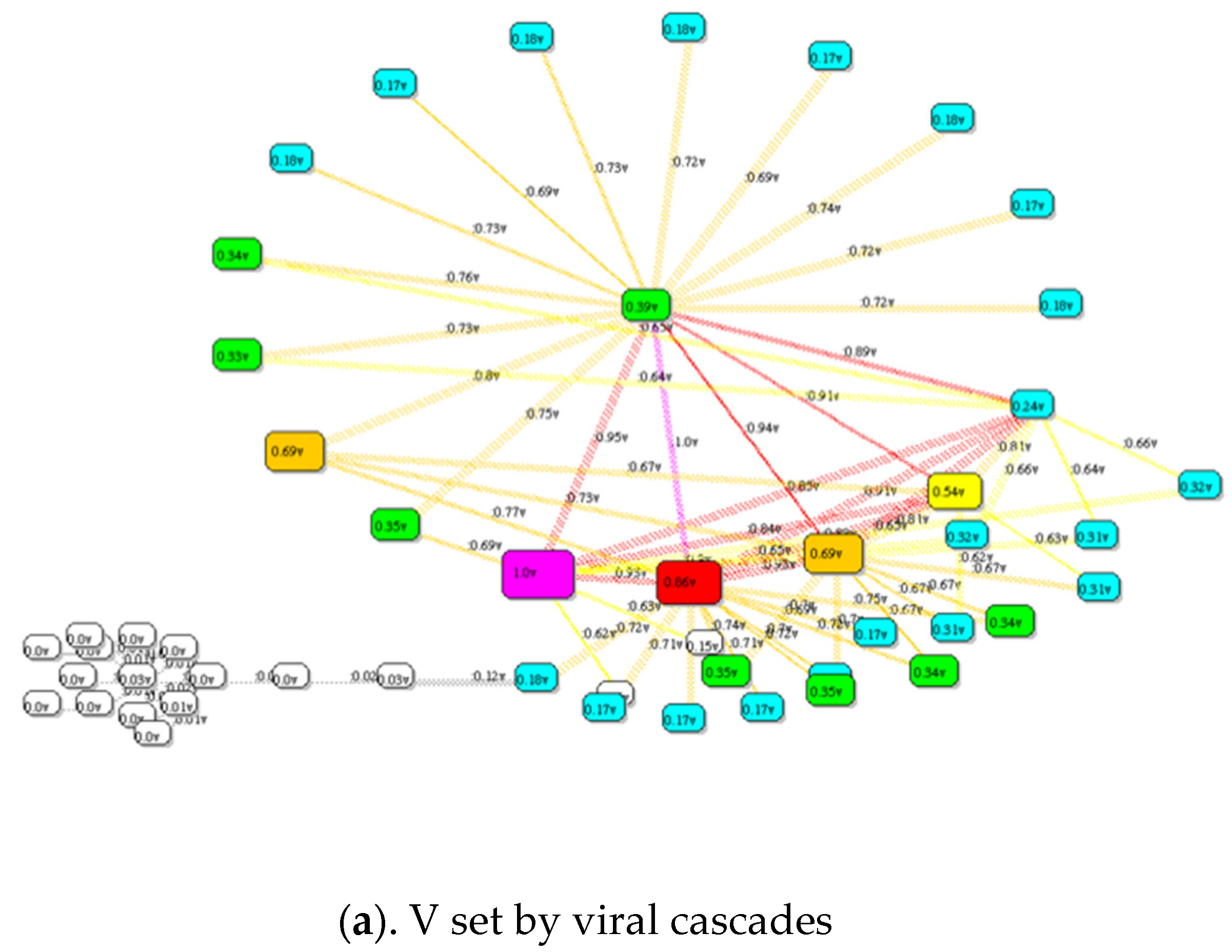
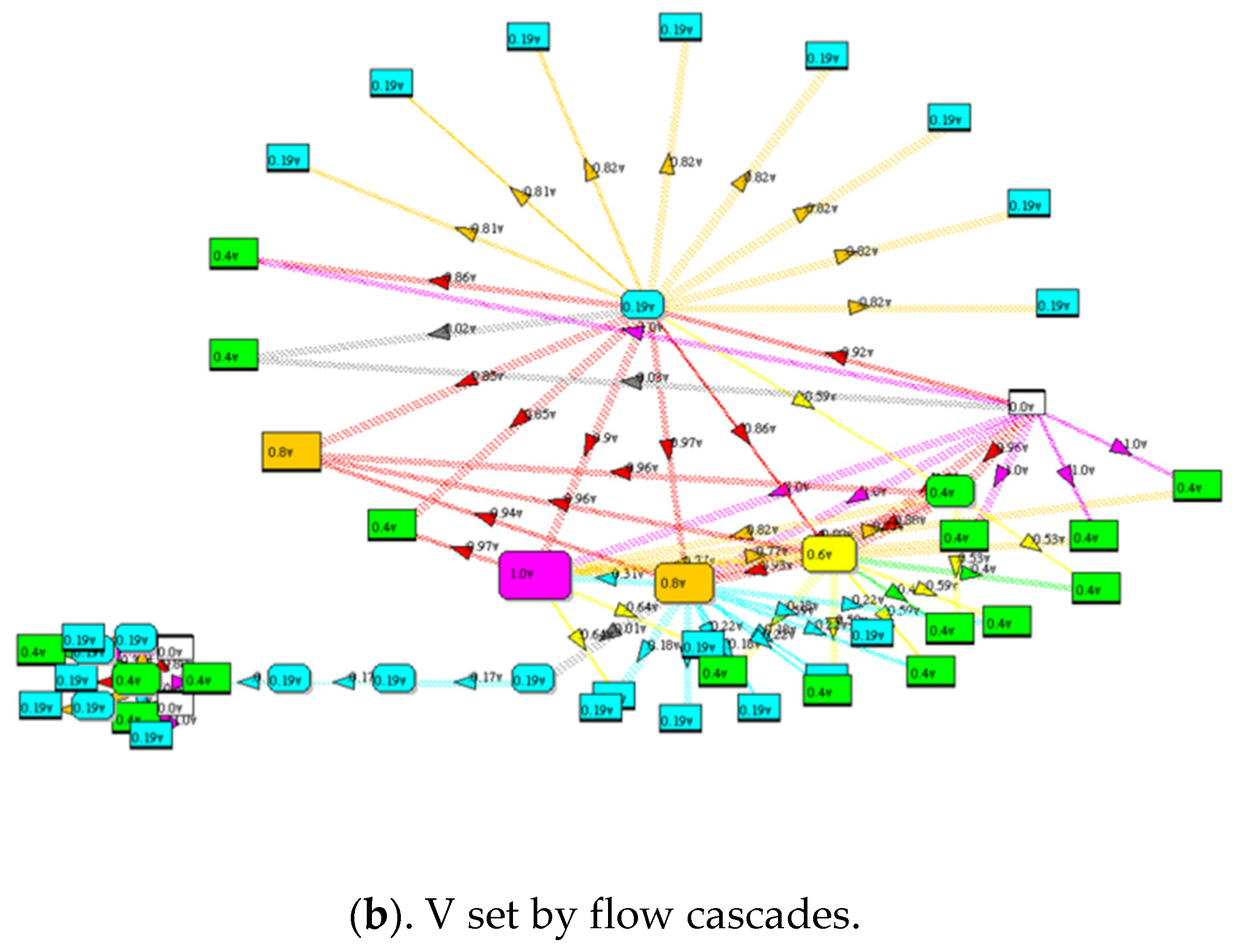
Domino effect failure is a form of viral cascade failure in a connected system that may lead to partial or complete collapse of the system. Cascading is a stochastic catastrophe observed in many real systems, e.g., traffic jams on highways, spread of contagion in a population, and software virus in a communication network. We examine two types of cascades—viral that fail due to adjacent actors failing, and flow that fail due to stress caused by overloading nodes and links. Viral cascades propagate via neighboring assets, while flow cascades propagate via non-contiguous assets that “break” due to redirected flows resulting in overloading.
1.2. Exceedance and Risk
A stochastic catastrophe K exceeds consequence x with probability EP(x), which is the likelihood that a system failure of size x is greater than or equal to x. EP is the exceedance probability of partial or complete collapse due to an initial fault at the seed asset that propagates through the system represented as a network [1]. Let X = [x1, x2, … xk]; xi > 0 be a monotonically increasing sequence of consequences xi < xi+1. Given frequency histogram of past failures due to stress, true EP is a monotonically declining distribution, as follows:
Note than x1 > 0, EP(xi) ≥ EP(xi+1) and EP(x1) . Thus, EP is a long-tailed distribution that monotonically decreases from 1.0 to a small fraction, EP(xk) = Pr(xk). See Figure 2 and Figure 3 for examples.
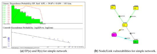
Figure 2.
Simulated viral cascading of the links of the simple directed network in Figure 1 produces a green exceedance probability EP(x) with q = 0.97 and red risk R(x) curve with MPL as its maximum point. A seed link is selected randomly 10,000 times within 5 trials. (a). Plot of exceedance probability in green, the risk in red, and a logarithmic plot of the exceedance probability showing linear (power law) fit to EP, with exponential cutoff. (b). A heat map of the directed network showing V used in the simulation of viral cascades. Nodes/links are heat map colored according to vulnerability. Consequence vector X is not shown: X = {100, 100, 100, 100, 100} for links and {100, 100, 200, 100, 100} for nodes.

Figure 3.
Illustrations of exceedance as a power law and risk derived from the exceedance probability curve. (a). US power grid risk versus consequence in terms of loss of kilowatt-hours of energy recorded over 10 years from 2007–2017. (b). Internet risk versus consequence in terms of breached sites recorded over 18 years from 2004–2022. The dotted line is the OLS fit to a power law.
Exceedance probability is of major concern to engineers and insurance companies, as opposed to simple probability Pr(x), because it represents the worst-case consequence. If consequence is measured in dollars, x, then EP(x) is the probability that financial losses will equal or exceed x dollars.
An example of exceedance probability applied to cascading in a network is shown in Figure 2. This simple directed network has two source nodes and one sink node, hence viral cascading may occur going forward along the directed links with probability given by vector V. Given a vector of consequences per node/link for all nodes and links, simulation may be used to determine the number of times each node fails and in turn to calculate the exceedance probability and risk.
Risk R(x) is expected loss associated with a stochastic catastrophe S defined as the product of loss and EP of loss:
R(x) = x EP(x); x is consequence = loss in dollars, casualties, kilowatt-hours, etc.
Risk is calculated by multiplying the x-axis (consequence) and y-axis EP along the EP(x) curve, see Figure 2.
In many cases, EP is a power law, or approximately a power law, especially for small values of V. Plotting log(EP(x)) versus log(x) as shown in Figure 2, yields the exponent of the power law, q. Since power laws are fractals, q is sometimes called the fractal dimension of the catastrophe. The purpose of plotting log(EP(x)) versus log(x) is to find q. As shown below, the determination of q < 1 is significant because q = 1 represents a tipping point [1].
Figure 3 illustrates the use of exceedance as a power law in the real world. The exceedance probability of a power grid outage obeys a power law with fractal dimension q = 0.46 indicating high risk due to an extremely long tail. The cyber exploits of 2015 show less exceedance (q = 0.97) and risk, but still relatively high. Note that the measure of consequence is different in each case, but the same mathematical analysis applies.
The parameters of the basic equations of catastrophe are obtained experimentally or by simulation:
Maximum Probable Loss, MPL = [2].
Note that these are idealized models and must be used with caution. In most cases where the approximation is poor, the exceedance probability obeys a power law with exponential cutoff:
We present results only for the pure power law case, which is suitable for values of V less than 0.5 and typical network structures. The EP(x) approximation becomes worse with values of V greater than 0.5. Keep in mind that even when EP(x) is not strictly a power law, and q is only an approximation, it is still useful as an indicator of intensity of risk and resilience.
Resilience Z follows from EP(x), R(x), MPL and fractal dimension q. We develop three measures of Z, below.
This will be our entry point into a general theory of catastrophes. With these elemental properties of complex systems in tow, we can rigorously define metrics for quantifying risk and resilience—the primary goal of mathematics of catastrophe. The steps are:
- Construct a network representation of the system including connectivity.
- Assign values of V and X to the node and link assets. V is a vector of probabilities and X is a vector of consequences.
- Run 10,000 simulations of viral cascading following a randomly selected node or link and count the number of times each node/link is faulted. [Run 5 trials of 10,000 each to obtain confidence levels].
- Calculate EP(x), R(x), and MPL.
- Calculate OLS fit of a power law to EP(x) to obtain the fractal dimension.
- Use the fractal dimension and MPL to compute resilience Z.
2. Materials and Methods
Two landmark developments provide us with a foundation for the mathematics of catastrophe—the seminal works of Per Bak and Charles Perrow [1,3,4,5,6,7]. Bak is known for his theory of punctuated equilibrium based on self-organized criticality, SoC, and Perrow for his Normal Accident Theory, NAT. We will show that SoC influences risk and resilience, and NAT suggests using network science as the basis of representing complex systems such as the power grid, water systems, and communication networks.
Given a network S containing nodes and links each with vulnerability: consequence pair V and X, we construct a mathematical model of EP, R, and ultimately resilience Z. We show that these properties depend wholly on V, X, and the spectral radius r of S. To compute EP, we use simulation of the network under stress causing one or more nodes/links to fail. In the remainder of this paper, two types of stress are considered, although the mathematics is easily extended to others: viral cascades and flow cascades.
2.1. SoC and NAT
The definition of self-organized criticality existed in the lexicon long before Per Bak rigorously defined it in the late 1980′s [4,5,6]. For example, Friedrich Hayek observed self-organization in economic systems, calling it “spontaneous order”, which is perhaps a better name, because self-organizing systems are systems that transition from disorder to order, over time. That is, a structure with greater order emerges with lower Shannon entropy over time. Initially, systems may appear without any predetermined order, or perhaps with a predetermined order but also with stresses that force it to find a new stable order. Over time, they conform to the stress/force and some form of structure emerges, often without a plan. Thus, complex systems evolve into self-organized systems, and as a result, they may become increasingly brittle and fragile.
The internet is a clear example of order emerging from disorder; structure emerging from less structure [8]. Originally designed to be “flat” in the sense of equal access and evenly distributed connectivity from anywhere, the internet is now a highly structured system of relatively few major (e-commerce) hubs and many single connections (consumers). It has evolved from a radically distributed network of computers to a radically centralized network of servers called “the cloud” [8,9]. Entropy has been reduced and structure is extreme.
Node degree is the number of links connecting the node. Degree distribution H(d) is the histogram constructed by counting degree frequency H versus degree, d. The node with the highest degree (most connections) is called the hub and has degree equal to dHub. H(d) is a binomial distribution for a random network, and a power law for a scale-free network [10].
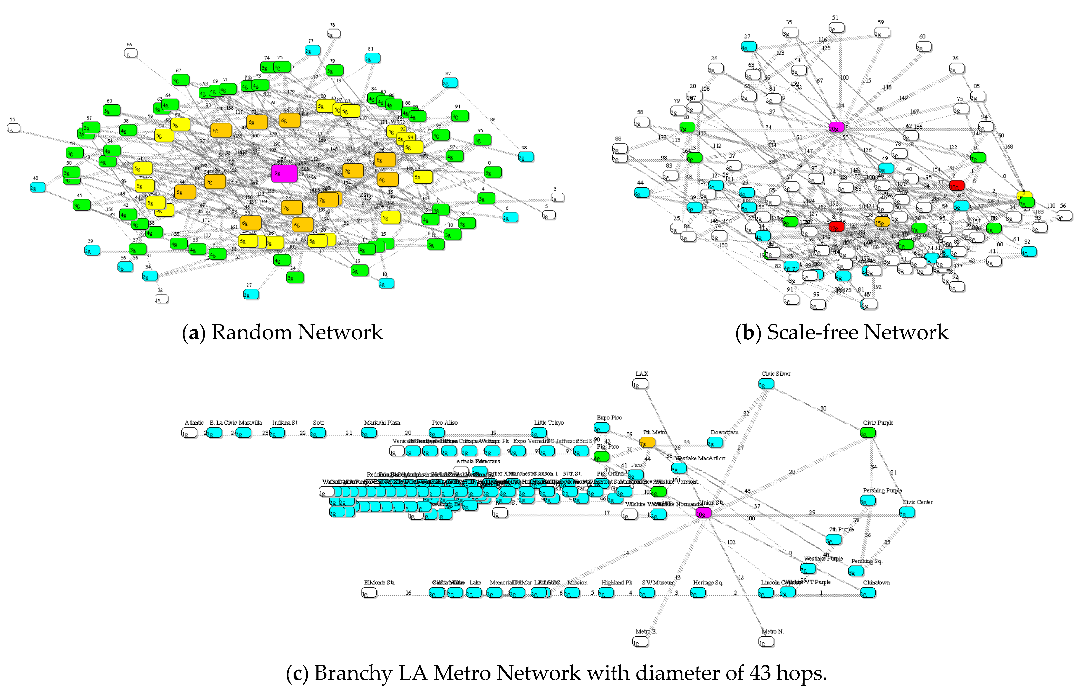
We equate the spectral radius of network S with SoC. Spectral radius is the largest eigenvalue of connection matrix M. As the number of links increase, so does spectral radius . More importantly, also increases with structure. For example, two networks with identical number of nodes and links exhibit different values of spectral radius due to the difference in their structure as indicated by degree connectivity, see Figure 4.

Figure 4.
(a). Random structure with 100 nodes and 197 links; spectral radius = 4.66, branchy = 2.58. (b). Scale-free network with 100 nodes and 197 links: spectral radius = 7.18, branchy = 0.84. (c). Branchy LA Metro network with 117 nodes and 127 links: spectral radius 3.69, Branchy 11.65. It is the recognition that structure matters, illustrated in this paper, that partially determines risk and resilience. Nodes are heat map colored to indicate connection degree.
A more general measure of structure is branchy versus the inverse bushy. Networks with large diameter relative to spectral radius are considered branchy. (Diameter is the longest distance between two nodes, where distance is measured in hops). In general, branchy networks are more resilient than bushy networks.
Figure 4 compares a random network, i.e., one constructed by randomly selecting two nodes to connect each of m links, a scale-free network with identical number of nodes and links, but different structure, and the LA Metro network with extreme structure in the form of large diameter [10,11]. The three networks are clearly ranked according to disorder, aka structure, as follows: Random, scale-free, and branchy LA Metro.
Bak realized that systems become more brittle and fragile as they self-organize over time. Hence self-organization and aging are related: old systems lose resilience as self-organization takes over, due largely to attempts to optimize performance, make modifications, or simply because of neglect. Efficiency is often the major cause, a realization that efficiency experts do not enjoy facing because it implies cost [1]. The three networks in Figure 4 can be ranked in terms of branchy resilience (from high-to-low) as follows: branchy LA Metro, random, and scale-free.
Bak’s contribution was to notice that catastrophic failures accumulate potential along with self-organization. That is, as systems represented as a connected network of nodes and links become increasingly structured, they also become increasingly fragile and prone to failure. He equated self-organization with “consequence potential”.
Self-organization is potential for catastrophic failure and increases consequence, exponentially.
About the same time Per Bak was developing the theory of self-organized criticality and its consequent system collapse, Charles Perrow was developing a similar theory of organizational collapse [10]. Perrow asked, “Why do systems collapse?”. His answer was, “Collapse is a failure of management.” Fragility is a sociological artifact—it is due to poor organization and a series of little “normal” mistakes made by people. In fact, the little mistakes occur in a series, one following another, until the compound effect is disastrous.
This sounds familiar in the case of COVID-19 pandemic. It is the little mistakes that compound and build up into a sizeable disaster. First, leadership failed when it did not recognize the magnitude of the threat. Next, preparations for the eventual avalanche of infected cases were woefully inadequate, followed by a weak roll-out of vaccines after the herculean development task. One normal accident after another snowballed into a global disaster of epic proportions.
However, upon deeper analysis, Perrow’s theory of NAT says something about complex systems that defied simple explanation at the time. NAT explains how an unseen force is responsible for holding a system together, or not. This coupling force is the glue that makes a conglomeration of parts a system. It is the coupling that matters. In addition, if the coupling comes apart, the system fails.
Perrow did not quantify this force, but he attributed coupling to a series of mistake—both technical and managerial—that compound into a big event such as the Three Mile Island Nuclear disaster described in detail in his book. Disasters, according to NAT, are the result of a series of little mistakes that propagate faults via coupling culminating in collapse. Moreover, the size of the failure snowballs—it becomes larger with each little mistake. Perrow’s observation paved the way for representing systems as complex networks. This observation concurs with Bak’s theory of self-organization.
Ultimate consequence of failure grows with each small fault because of the presence of a coupling force—an undefined element according to Perrow. Coupling is modeled as connectivity of nodes in a network, and connectivity determines topology.
Per Bak would have agreed with Perrow had he been aware of his work, and furthermore, Per Bak would have been able to quantify the series of mistakes, one piled in top of the other, culminating in a disaster. In fact, the likelihood of a major event following a series of improbable small events is the product of probabilities of each event in the series. This, and other forms of conditional probability, leads to a long-tailed distribution describing the exceedance probability of the disaster. Perrow says the source of fragility is a sequence of events leading up to collapse, and Per Bak showed that the exceedance probability obeys a long tail distribution. They both attributed the catastrophe to connectivity within the system.
2.2. Viral vs. Flow Cascades
SoC and NAT applies especially well to viral cascade failures where the failure in one node/link propagates with probability v to adjacent nodes/links. Every node and link has an associated vulnerability and consequence, x; V and X are vectors containing vulnerability probabilities and consequences. Given a seed node/link failure, subsequent faults propagate through S in a domino effect called a viral cascade. The size of the cascade is measured in terms of the fraction of faulted nodes/links after propagation dies out. The fraction of faulted nodes or links varies stochastically. Repeated simulations of viral cascades produce an exceedance probability, EP(x) and risk profile R(x). A long-tailed exceedance probability may be approximated by a power law with fractal dimension, q. Hence, EP(x) and R(x) are functions of vulnerability V, consequences X, and network topology represented by spectral radius .
For viral cascades, risk increases with an increase in vulnerability V and a decrease in fractal dimension q of the exceedance probability, EP(x), e.g., as q declines, the tail becomes longer and fatter, hence R(x) is greater. This leads to the first axiom of catastrophic failures: Catastrophic failure depends on the weakness of system components (nodes and links) and structure , both.
Viral cascade risk and resilience decline with increasing branchy, which offsets spectral radius in most systems.
Complex systems that support commodity flows such as supply chains, road networks, electrical power grids, cyber systems, etc. fail differently due to breaks in the flow. For example, in a power grid, a tripped transmission line in one part of the network may cause an overload in another, non-contiguous part of the network. The non-contiguous line subsequently trips due to the surge and overload, and so forth. This domino effect is called a flow cascade because it propagates via overloading rather than by tripping adjacent nodes/links.
We treat flow cascades separately from viral cascades, but the mathematics is similar. Consequence is measured in loss of flow. The exceedance probability curve and risk are still approximated by a power law and probable loss, EP(x) and R(x).
Resilience Z is tolerance for faults in nodes/links leading to loss of flow. In general, we find that loss of flow is correlated with number of blocking nodes/links, where a blocking node or link is one whose removal segments the network into disconnected components. Removing a blocking node/link establishes one or more islands preventing flow from one island to any others.
2.2.1. Quantifying Viral Cascade Resilience
Normal accidents happen every day, and once in a while they have huge consequences. In fact, the longer a “normal accident” hides in a system leading to subsequent faults, the bigger is the catastrophe [5,6]. Faults increase damage as they pile one on top of the other. A loose bolt combined with a leak in the cooling system conspires with managements desire to cut costs or optimize performance, all leading to the big collapse. Perrow couldn’t explain his theory analytically, but it sounded a lot such as self-organized criticality where the coupling force is any force driving a connected system to self-organize. In addition to the system’s parts, their connectivity plays a major role, too. This was perhaps the first mention of connectivity and structure as a partial cause of collapse.
There is a relationship among the variables in our model: V, X, spectral radius r, and fractal dimension q. This is not surprising because network topology, V, and X are independent variables, and EP, R, and MPL are dependent. The relationship can be determined by performing simulation experiments.
For viral cascades, we run a series of simulations varying V and measure the resulting fractal dimension of EP for each value of V, see Figure 5. Fitting an OLS straight line to a plot of log(q) versus the product (k ), produces parameters b and k from the following empirical relationship:
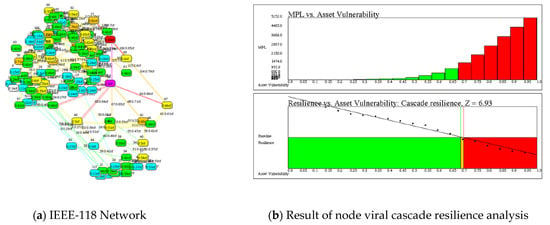
Figure 5.
Resilience of the network representing the IEEE-118 test power grid with 118 buses (nodes) and 180 power lines (links) [12]. (a) Network with the frequency of cascading cF shown as a colored heat map and numerical values. (b) Upper graph shows MPL risk for each value of vulnerability from 0 to 1.0; Lower graph shows resilience declining with respect to v; and the line crossing at log(q) = 0 yields resilience, Z = 6.93 when q = 1.0.
In Figure 5 we obtain:
Note that q = 1 is a tipping point for R(x) = xEP(x) = x(1−q), because R(x) is unbounded for q < 1 and bounded for q ≥ 1. When q = 1, log(q) = 0—the tipping point. Let v0 be defined when q = 1:
log(1) = 2.17 − 3.14 v0 = 0;
v0 = 2.17/3.14 = 0.693
Now define viral resilience Z in terms of v0, thus:
Z = 10 v0 = 6.93
The logic of selecting normalized viral cascade resilience, Z in terms of the zero-crossing point along the v axis is traced to the significance of the zero-crossing point:
When q < 1: R(x) monotonically increases and becomes unbounded
q ≥ 1: R(x) monotonically decreases approaching zero.
Therefore, q = 1 is a tipping point between bounded and unbounded risk and v0 marks that point.
One is tempted to declare q = 1 the critical point at which catastrophe changes phase from bounded to unbounded consequence [12]. Hence, resilience is tolerance for viral cascading that approaches the change in phase from mild to extreme collapse. The measure of resilience Z is the tipping point along the vulnerability axis where the catastrophe changes phase from mild to extreme.
2.2.2. Quantifying Flow Cascade Resilience
The following measures of resilience are two of many possibilities for defining resilience. First, resilience depends on nodes and links whose removal segments the network into components, called blocking nodes/links. Flow from one component cannot reach other components if a blocking node/link is removed or damaged. Second, a fault is assumed to occur when flows overload nodes/links and “trip” them due to overloading. This is determined by computing a flow ratio, which is a measure of overloading. Resilience overloading is computed by measuring the decline in MPL versus flow ratio for a range of loads exceeding capacity of nodes/links.
2.2.3. A Simple Measure of Resilience Based on Blocking Nodes/Links
When a blocking node or link is removed from network S, it segments S into isolated components such that it is impossible for flow to reach other components from within a component. Network components are connected subsets of S unless one or more blocking nodes/links is removed or damaged. Every node can be reached by any other node by hopping from one to another via links.
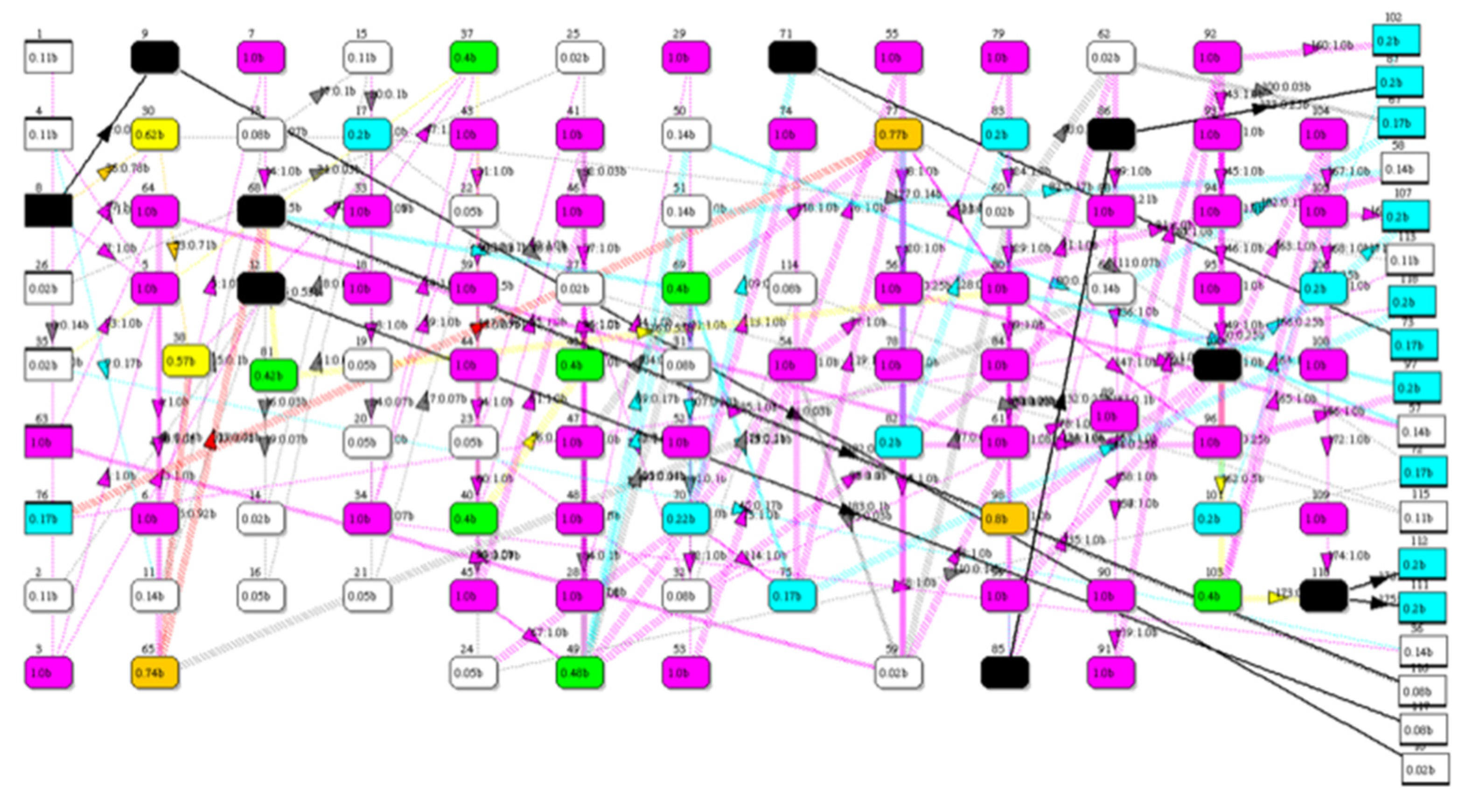
Let B be the number of blocking nodes and links in S with (n + m) nodes and links. Then blocking resilience is defined as ZB ). Alternatively, this is a measure of redundancy, because it is the fraction of nodes that provide strong connectivity. Retaining strong connectivity implies alternate paths for flows through the network. These alternate paths are what makes the network redundant and therefore resilient.
Figure 6 illustrates this form of resilience, measured on a scale of 0 to 10.
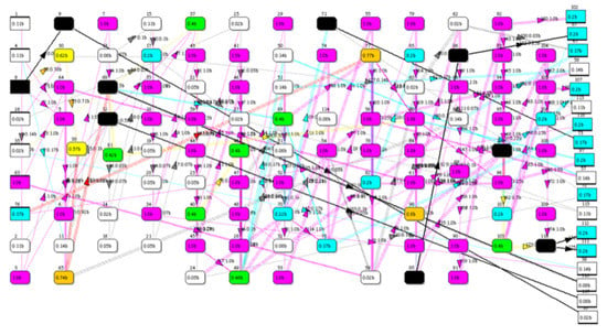
Figure 6.
Heat map of IEEE-118 power grid test network with n + m = 304; the 9 blocking nodes and 9 blocking links are colored black, and all other nodes/links are assigned a bottleneck rating from 0 to 1.0 (and color code) based on their network topological betweenness. The network is drawn with sources on the left and sinks on the right.
2.3. Resilience Based on Overloading of Nodes/Links
In the previous section we developed risk and resilience equations for fault propagation in components of a system represented by nodes in the network. In this section, we develop risk and resilience equations for the loss of flow due to faults in connections represented by links in a directed network. The mathematics look similar, because it is based on long-tailed exceedance probability. However, the definitions of consequence and resilience are quite different.
Directed networks contain source and sink nodes with capacity defined as the maximum flow allowed through each node/link. We are particularly interested in links, but flow capacity of nodes may also be analyzed by measuring the difference between the flow of a commodity such as water, gas, oil, and electrons from source to sink when under stress. Specifically, stress manifests itself as loss of flow at the sink nodes relative to total input at source nodes. Therefore, a measure of risk is the expected loss of output flow relative to total of flow inputs:
Consequence, x = total input from all source nodes—total output at all sink nodes
Consequence x is equal to 0, if flow is not disrupted, because it is assumed there is no loss of flow without a fault. When a disruption such as a congested or broken link occurs, the output from all sink nodes sums to something less than the total input from all source nodes, hence percentage of consequence is greater than zero, but less than or equal to 100%.
If the flow network contains enough redundancy in the form of alternate paths, it may adapt by re-routing flow through alternate paths. If no alternate path exists, and the links tolerate flows greater than they were designed for—an overload occurs—and the consequence may still be zero. Thus, two alternatives are possible, (1). re-routing, and (2). overloading. Otherwise, total output flow declines with corresponding consequence greater than zero.
With this definition of consequence, we obtain an exceedance probability and risk curve by simulation of single link failures, one at a time for all m links. For each link in the network, we simulate a fault in the link and re-route around it, if possible. We then calculate the output flows, compute consequence, and plot exceedance and risk versus consequence to obtain fractal dimension and MPL. This is illustrated in Figure 7 for the IEEE-118 test grid.

Figure 7.
Flow analysis of the IEEE-118 power grid test network. (a). The network organized with sources on the left and sinks on the right. (b). EP(consequence), R(Consequence) and MPL derived from faulting one link at a time and measuring the resulting cascade. Total flow in is 4100, MPL is 72.74, and q = 1.19. Nodes/links heat map colored according to their capacities.
Exceedance declines precipitously as might be expected when a link fails, cutting off flow through the link and possibly downstream. Figure 7 shows MPL = 72.74 of total flow equal to 4100, and an exceedace probability power law with fractal dimension of q = 1.19. This result holds for a single link fault, i.e., L-1 stress testing of links.
In many flow networks re-routing leads to other links failing because of overloading. This is a form of cascading experienced in power grids, for example. In this case, resilience is the ability to tolerate overloading and continue to function. That is, flow resilience shows up as a decline in MPL as links overload. We quantify overloading as the ratio of flow to capacity:
And cutoff is defined as the maximum flow ration tolerated by nodes/links. If simulated flow exceeds this cutoff ratio, it is considered a fault. Hence, resilience depends on tolerance for a flow ratio greater than one. Plotting MPL risk versus overload yields a declining risk curve with slope . A rapid decline in indicates greater resilience. The value of Z is normalized between 0 and 10 by computing the ratio of areas, see Algorithm 1.
| Algorithm 1: N-k Z Resilience |
Sub-algorithm A: N-k link fault simulation:
|
Note: Algorithm 1 applies backpropagation similar to backpropagation used to train artificial neural networks. Flows are computed backward through the network from sink nodes to source nodes by repeated matrix multiplication. Overloaded links are removed from the BACKPROP matrix and flow rations recomputed for the remaining nodes. Then a FORWARDPROP matrix is applied to compute the flows from source nodes to sink nodes using (possibly) alternate pathways through the network.
An N-k link cascade occurs when a seed link fails, flows are re-routed around the failed link possibly resulting in overloading subsequent links. If overloading causes a link to fail, the fault propagates to other non-contiguous links, which may also overload and fail. Thus, an avalanche of faults spreads through the network until no subsequent overloads/faults occur. Exceedance and risk can be calculated in a manner similar to viral cascading, however, resilience is a different matter. Resilience in this case, is tolerance for overloading.
The measure of flow resilience is based on tolerance for overloading links. By varying the allowed flow ratio from 1.0 to some upper amount maxCutOff and calculating the resulting MPL value, we can plot MPL versus flow ratio. If MPL decreases with increase in flow ratio, it must be due to tolerance for overloading. Thus, the amount of decrease versus flow ratio is a measure of resilience.
Figure 8 illustrates resilience of IEEE-118 power grid test network under overload stress. MPL is obtained from EP(loss), where losses are ranked, and R(loss) computed from loss * EP(loss). This involves repeating calculation of loss for each link, taken one at a time. Keep in mind that faulting a single link may result in k link faults.

Figure 8.
Resilience of the IEEE-118 power grid test network. (a). A colored heat map of flow ratios obtained from removal of one link and re-routing. This suggests “hot spots” in the network that are likely to overload when stressed. (b). Calculating flow resilience Z = 5.66 out of 10.0.
The stress test is carried out as follows:
Flow resilience is resistance against collapse due to cascading link failures caused by overloading. If overloading occurs without a fault, MPL should decrease, as it does, see Figure 8b. In fact, a rapid decrease it MPL versus overload cutoff value, signifies greater resilience than a gradual or no decrease. Thus, Z is the ratio of MPL(cutoff) to maximum MPL summed over all values of monotonically decreasing MPL.
3. Results
We performed simulation studies on a select collection of systems with network representations spanning a wide range of properties, see Table 1. Artificial networks: Binary Tree, Star, Random, and Scale-free were chosen because of their varied topologies, i.e., spectral radius ranged from 3.00 to 6.72. Real-world networks LA Metro (the Los Angeles light rail system), IEEE-118 test (IEEE power grid for test purposes), Industrial Control System (computer network for controlling power station), 911 Terrorist (the social network formed by the 911 terrorists). These were selected because they offer a wide range of systems with varied topologies, i.e., spectral radius ranging from 3.69 to 8.62. Correlations with each metric versus viral resilience are shown at the bottom of Table 1.

Table 1.
Properties of a select collection of networks with widely variable structure. Fractal dimension obtained by simulations with v = 0.20. Correlations are with viral resilience Z.
3.1. Viral Cascades
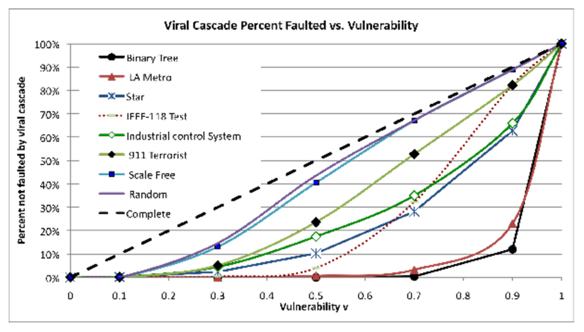
Figure 9 shows how these networks respond to viral cascading versus vulnerability. The likelihood that a certain node is faulted by an adjacent node is highly correlated with the number of connections to the node, i.e., node degree. Intuitively this makes sense, because the number of times a node is contacted by a (possibly faulted) adjacent node is equal to the number of links connecting the node. For the collection of networks in Figure 9, the average value of correlation with fault percentages vs. degree is 86%.
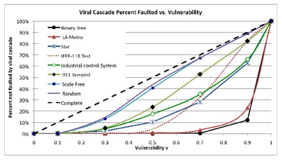
Figure 9.
Percentage of nodes faulted versus vulnerability V. Correlation = 0.86 on average. Branchy networks (Binary tree, LA Metro, IEEE-118 Test) tend to spread faults less than bushy networks, hence they are more resilient.
Given that V is identical for all networks and the number of faulted nodes is normalized to a percentage of the total, the only difference among the networks is their structure. Hence, the correlations with viral resilience range from mild (0.55) to strong (0.78). In particular, branchy, spectral radius, and blocking Z are good predictors of resilience. Networks may be categorized according to how “bushy” or “branchy” they are with branchy a fair predictor of viral resilience.
The most branchy networks in Table 1 are IEEE-118 Test, LA Metro, and Binary tree. The bushy networks are Scale-free, Star, and 911 Terrorist. Thus, for the collection of networks in Table 1, the results are summarized as follows:
Spectral radius, branchy, and number of blocking nodes/links are three meaningful properties of viral cascading in networks that correlate with risk and resilience, independent of network size. Branchy networks are more resilient than bushy networks due largely because of network diameter.
3.2. Flow Cascades
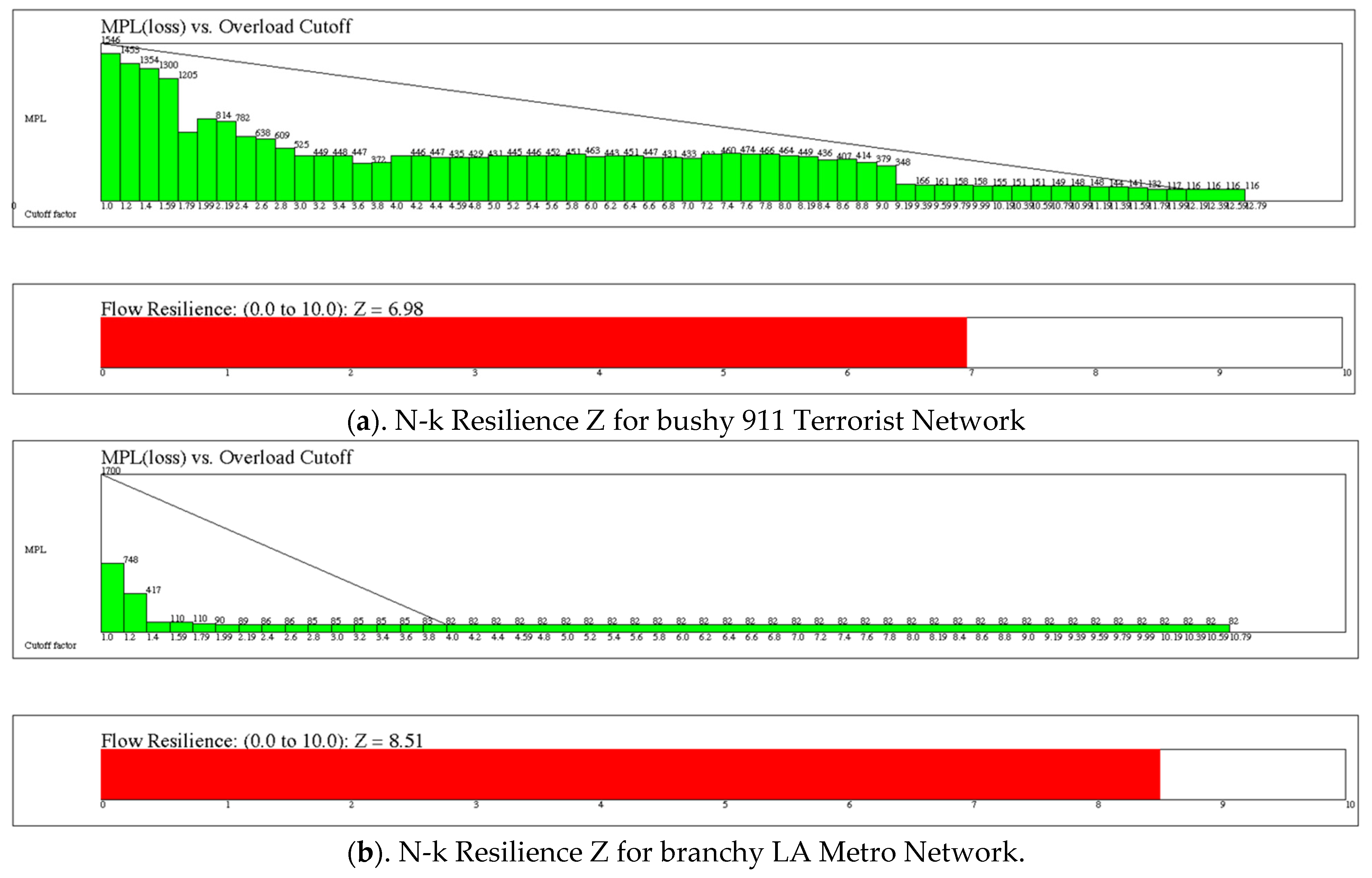
In this section we give results for three stress tests: (1). Link Minus One (Link-1) testing where the effect on flow from sink-to-source nodes is simulated by removing a single link, (2). Link Minus K (N-k) testing where the effect of removing one link causes a cascade of other links exceeding their capacity to also fail with corresponding decrease in flow at the sink nodes, and (3). Flow resilience (N-k Z) the network’s tolerance for overloading under N-k stress testing. The difference between (1) and (2) is that the simulation considers cascading faults in (2), but only the effect of a single link faulting in (1). The difference between (2) and (3) is in the overflow ratios tested—(2) tests for overflow ratio equal to 1.0, while (3) tests for a range of overflow ratios from 1.0 up to maxCutOff as specified in Algorithm 1. The results for applying Algorithm 1 to bushy network 911 Terrorists versus branch network LA Metro are shown in Figure 10. In general, Branchy networks are more flow resilient than bushy networks, but this is tempered by the number of blocking nodes/links.

Figure 10.
(a). Flow resilience Z test for 911 Terrorist network with bushy of 1/0.58 = 1.72 and resilience of 6.98. (b). Flow resilience test for the LA Metro network with branchy of 11.65 and resilience of 8.51.
The N-k Z metric is a normalized 0 to 10 measure of resilience based on the rate of decline in MPL risk as overloading is allowed to increase without faulting the link. N-k Z is calculated by Algorithm 1, above, by simulating flow from source-to-sink following a link removal followed by a cascade of overloaded link failures—number (2), in the previous paragraph. The simulation is carried out for each overload cutoff ratio ranging from 1 to maxCutOff (set by user).
Table 2 summarizes the results for flow cascades. Note that Link-1 MPL is typically low and N-K MPL is typically high. This highlights the difference between a single failure and an avalanche of failures as a fault in one link propagates to others. However, Link-1 MPL is mildly correlated with N-k resilience Z signaling the relationship between one link fault and an avalanche of faults. Spectral radius has the highest correlation value for this collection, indicating that structure plays a role in flow resilience. In fact, the correlation coefficient for spectral radius versus Link-1 MPL is 0.62 (not shown).

Table 2.
Results for flow cascade simulations on the collection of networks. N-k Z is only mildly correlated with the properties listed.
3.3. Prediction
In addition to analyzing macro-level effects of viral and flow cascading, one can model the impact of individual vulnerabilities of nodes/links on the future performance of risk and resilience by substituting simulation results in for V to estimate the likelihood of future failure, e.g., predicting where faults might occur. We illustrate this with viral and flow cascade node/link property cF:
cF: cascade frequencies based on simulated viral cascades
cF is a simulation-derived estimate of the probability a node/link will fail under stress. For viral cascading, the stress is a node/link fault. For flow cascading, the stress is an overloading caused by a node/link fault. In both cases, cF is considered a predictor of faults.
3.3.1. Using cF to Predict Future Viral Faults
Recall that viral cascading is an avalanche of faults emanating from a seed node/link and spreading until no additional nodes/links fail. Property cF(i) is the number of times node/link (i) fails when the simulated viral cascade is repeated t times:
If vector V is replaced with cF and the simulation repeated, a revised cF is obtained. Repeating several times gives a stable result whereby cF(i) no longer changes. Thus, cf(i) is the likelihood of node/link i failing in a viral avalanche. Figure 11a shows the results of applying this algorithm to the industrial control system network with an initial V set to 0.1 and substituting cF in place of V five times.
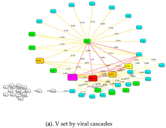
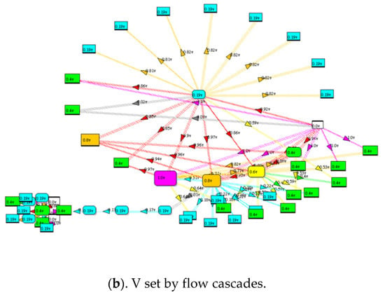
Figure 11.
Predicting future failure of nodes/links in a network is computed by simulating the number of times a node/link is faulted cF as illustrated here for the Industrial Control system network. Colored heat maps of (a) Result for t = 10,000 simulated viral cascades and (b) result for N-k link overload cascades.
3.3.2. Using cF to Predict Future Flow Overloading Faults
Flow cascades due to overloading nodes/links are simulated as described above. In addition, the number of times a node/link overloads cF is recorded during simulation. Each link is tested one at a time, potentially causing an overloaded node/link downstream. The results are shown as a heat map in Figure 11b.
4. Discussion
Complex systems modeled as networks with a single measure of catastrophe performance—either viral or flow cascading– pose a challenge to rigorous analysis. There are many faces of risk and resilience not addressed here. For example, scale-free networks have been reported as being much more resilient than random networks [6], based on random attacks on nodes. However, what if the attacks are not random and the links are the target? For the random versus scale-free network studied here, the results are that targeted attacks on the random network shows slightly more resilience against attacks on its largest-degree node than the scale-free network resilience against attacks on its hub node. The reverse is true for links: the scale-free network is more resilient than the random network with respect to random attacks on links.
The main equations developed by the author and used here have been shown to be robust enough to approximate viral and flow risk and resilience based on the long-tailed power law. This approach is possible because exceedance probability is long tailed by definition. However, the approximation becomes worse as vulnerability V becomes large. V should be less than 50% as a rule, but also the approximation becomes worse for extreme network topology such as a linear chain.
More important, simulations can identify the most likely nodes/links to fail under stress as illustrated by the simple predicted value of V for viral and flow cascades. Node degree is highly correlated with viral cascade failure, but the correlation does not follow for links. By counting the number of faults cF during simulation, one can estimate the likelihood of faulting under similar stress in the future.
The results presented here apply to vulnerabilities less than 0.5. This might be criticized for lack of accuracy and mathematical rigor. In fact, the power law extends to infinity, but networks are finite sized in terms of nodes/links. This may account for inaccuracies in the tail of the power law representation of exceedance probability. The model can be enhanced by considering an exponential cutoff parameter . Figure 3 illustrates this when q < 1 should produce an infinite value of MPL, but instead the finiteness of the networks in Figure 3 introduces an exponential cutoff.
Prior modeling of risk and resilience of networks under stress reported by Dudenhoeffer et al. [13] offer no mathematical foundations, but the treatment of infrastructure systems as networks is similar. In [14,15,16,17,18] various authors have studied very similar stresses on complex networks (viral and flow overloading), without a general mathematical foundation and metrics. Smalley et al. introduced the idea of using fractals to characterize catastrophic earthquakes [19]. Liu and Ji report analytic results for flow resilience (percentage of lost traffic with respect to network size and link failure probability) for hypothetical communication networks [20]. Woo introduced the use of MPL as a measure of risk and notes that there are many definitions of MPL risk [2]. We have added to the list by assuming exceedance is a power law. The algorithm for simulating flow cascades is an enhancement to the tree algorithm proposed by Bernabeu et al. [21], which is similar to the algorithm used in [12,22,23]. We extended these algorithms beyond electrical power grids to generalized networks and enhanced them to include resilience. Our main contribution is defining useful measures of resilience Z and predictive modeling through simulation.
5. Conclusions
Software for performing the simulations was developed in Java and assigned for commercial use to Criticality Sciences, (https://www.linkedin.com/company/criticality-sciences accessed on 4 August 2022) It has been used to analyze water networks, power grids, and industrial control systems. The major difficulty for users is collecting data—values of vulnerability and consequence. Users are not accustomed the quantifying consequence before a catastrophic failure happens and probabilities are mere guesses at best. For this reason, vulnerability is treated such as a computed value instead of an input value. For example, simulations of viral and flow cascades produce cF, which may be used for v.
It is difficult to generalize catastrophes, especially before they happen, but it is interesting to correlate potential consequences with network topology—a novel method of obtaining insight into what causes or magnifies failure. The generalizations are summarized, below.
Spectral radius, branchy, and number of blocking nodes/links are three meaningful properties of viral cascading in networks that correlate with risk and resilience, independent of network size. Branchy networks are more resilient than bushy networks due largely because of network diameter.
Flow resilience is correlated with spectral radius, blocking node/link resilience, and Link-1 MPL, but only mildly.
cF obtained by simulation is a simple measure of points of failure under viral and flow cascades.
Future work consists of development of algorithms for determining bottlenecks and congestion in networks. A bottleneck, for example, might be a node or link where flow is expected to become constricted. Congestion might be defined as a stochastically significant event where an overload is expected to happen because of topology. Surges may also lead to bottlenecks and congestion. In this work we have assumed a constant input flow over time. Future work might model diurnal variation in flow as a sine wave. For example, power grid flows change as much a 100% over a 24-h period.
Author Contributions
T.G.L. contributed all to this paper. All authors have read and agreed to the published version of the manuscript.
Funding
This research received no external funding.
Institutional Review Board Statement
Not applicable.
Informed Consent Statement
Not applicable.
Acknowledgments
Thanks to Criticality Sciences and CEO Susan Ginsburg for the use of NetResilience, the software tool used in the analysis.
Conflicts of Interest
The author is an advisor to Criticality Sciences, Inc.
References
- Lewis, T.G. Critical Infrastructure Protection: Defending a Networked Nation, 3rd ed.; John Wiley & Sons: Hoboken, NJ, USA, 2020; 500p. [Google Scholar]
- Woo, G. Natural Catastrophe Probable Maximum Loss. Br. Actuar. J. 2002, 8, 943–959. [Google Scholar] [CrossRef]
- Peter, J.D.; Lewis, T.G. Uncertainty. Commun. ACM 2019, 62, 12. [Google Scholar] [CrossRef]
- Bak, P.; Tang, C.; Weisenfeld, K. Self-organized criticality: An explanation of 1/f noise. Phys. Rev. Lett. 1987, 59, 381–384. [Google Scholar] [CrossRef]
- Bak, P. How Nature Works: The Science of Self-Organized Criticality; Copernicus Press: New York, NY, USA, 1996; ISBN 0-38-94791-4. [Google Scholar]
- Lewis, T.G. Bak’s Sand Pile: Strategies for a Catastrophic World; Agile Press: Williams, CA, USA, 2011; p. 382. [Google Scholar]
- Perrow, C. Normal Accident Theory; Princeton University Press: Princeton, NJ, USA, 1999. First published 1984 by Basic books. [Google Scholar]
- Adamic, L.A.; Huberman, B.A. Power-law distribution of the World Wide Web. Science 2000, 287, 2115. [Google Scholar] [CrossRef]
- Lewis, T.G. Regulation of Communications Sector Considered Harmful. Available online: https://cip.gmu.edu/2016/02/03/regulation-of-communications-sector-considered-harmful/ (accessed on 2 August 2022).
- Barabasi, A. Scale-Free Networks. Sci. Am. 2003, 288, 60–69. [Google Scholar] [CrossRef] [PubMed]
- Albert, R.; Jeong, H.; Barabasi, A. The Internet’s Achilles’ Heel: Error and Attack Tolerance of Complex Networks. Nature 2000, 406, 378F382. [Google Scholar] [CrossRef] [PubMed]
- Rahnamay-Naeini, M.; Wang, Z.; Mammoli, A.; Hayat, M.M. A probabilistic model for the dynamics of cascading failures and blackouts in power grids. In Proceedings of the 2012 IEEE Power and Energy Society General Meeting, San Diego, CA, USA, 22–26 July 2012; pp. 1–8. [Google Scholar] [CrossRef]
- Dudenhoeffer, D.; Permann, M.; Manic, M. CIMS: A Framework for Infrastructure Interdependency Modeling and Analysis. In Proceedings of the 2006 Winter Simulation Conference, Monterey, CA, USA, 3–6 December 2006; IEEE: New York, NY, USA, 2006; pp. 478–485. [Google Scholar]
- Watts, D.J. A simple model of global cascades on random networks Proc. Natl Acad. Sci. USA 2002, 99, 5766. [Google Scholar] [CrossRef] [PubMed]
- Motter, A.E.; Lai, Y.-C. Cascade-based attacks on complex networks Phys. Rev. E. 2002, 66, 065102. [Google Scholar]
- Holme, P.; Kim, B.J. Vertex overload breakdown in evolving networks Phys. Rev. E. 2002, 65, 066109. [Google Scholar]
- Moreno, Y.; Gómez, J.B.; Pacheco, A.F. Instability of scale-free networks under node-breaking avalanches Europhys. Lett. 2002, 58, 630. [Google Scholar]
- Zhao, L.; Park, K.; Lai, Y.-C. Attack vulnerability of scale-free networks due to cascading breakdown Phys. Rev. E 2004, 70, 035101. [Google Scholar]
- Smalley, R.F.; Chatelain, J.-L.; Turcotte, D.L.; Prévot, R. A fractal approach to the clustering of earthquakes: Applications to the seismicity of the New Hebrides. Bull. Seismol. Soc. Am. 1987, 77, 1368–1381. [Google Scholar]
- Liu, G.; Ji, C. Scalability of Network-Failure Resilience: Analysis Using Multi-Layer Probabilistic Graphical Models. IEEE/ACM Trans. Netw. 2009, 17, 319–331. [Google Scholar] [CrossRef]
- Bernabeu, E.; Thomas, K.; Chen, Y. Cascading Trees & Power System Resiliency. In Proceedings of the 2018 IEEE/PES Transmission and Distribution Conference and Exposition (T&D), Denver, CO, USA, 16–18 April 2018; pp. 1–9. [Google Scholar] [CrossRef]
- Dobson, I.; Carreras, B.A.; Lynch, V.E.; Newman, D.E. Complex systems analysis of series of blackouts: Cascading failure, critical points, and self-organization. Chaos 2007, 17, 026103. [Google Scholar] [CrossRef] [PubMed]
- Ren, H.; Dobson, I.; Carreras, B.A. Long-Term Effect of the n-1 Criterion on Cascading Line Outages in an Evolving Power Transmission Grid. IEEE Trans. Power Syst. 2008, 23, 1217–1225. [Google Scholar] [CrossRef]
Publisher’s Note: MDPI stays neutral with regard to jurisdictional claims in published maps and institutional affiliations. |
© 2022 by the author. Licensee MDPI, Basel, Switzerland. This article is an open access article distributed under the terms and conditions of the Creative Commons Attribution (CC BY) license (https://creativecommons.org/licenses/by/4.0/).


