Polynomial Annuities

Abstract

We use a payment pattern of the type $\{1^k,2^k,3^k,\dots \}$ to generalize the standard level payment and increasing annuity to polynomial payment patterns. We derive explicit formulas for the present value of an n-year polynomial annuity, the present value of an m-monthly n-year polynomial annuity, and the present value of an n-year continuous polynomial annuity. We also use the idea to extend the annuities to payment patterns derived from analytic functions, as well as to payment patterns of the type $\{1^r,2^r,3^r,\dots \}$, with r being an arbitrary real number. In the process, we develop possible approximations to $k!$ and for the gamma function evaluated at real numbers.

1. Introduction

An annuity is a payment structure where a series of payments is made at various instants of time, with the objective spreading out a single lump-sum payment over a period of time. A level annuity is a payment structure where the same amount P is paid at all future instants of time. Typical annuity payments are finite in number over a finite period of time. When the annuity payments are made without a time limit (payments forever), then it is called a perpetuity. An important calculation for a given annuity payment structure is to compute the present value of the annuity, using the idea of the time value of money. For finite-time annuities, the future value at the end of the time period is also of interest. Annuity calculations are part of a subject called the theory of interestin actuarial mathematics (see, e.g., [1,2,3,4]).

The idea of an increasing annuity, with a payment pattern of $\{1,2,3,\dots \}$ is a standard variation on a level payment annuity, which is a topic discussed in interest theory (see, e.g., [1,2,3,4]). The present value of an increasing immediate annuityis typically denoted by ${\left(Ia\right)}_{\overline{n\hspace{.2em}|}i}$. Such an annuity is modeled after a linear increase in payments. Along the same lines, a geometric annuity is one that has an exponential payment pattern of $\{1,(1+g),{(1+g)}^2,\dots \}$, which is also a standard topic in interest theory. Formulas for present and future values of annuities and perpetuities with such a linear or exponential payment pattern can be easily derived using basic principles.

A payment pattern of the type $\{1^k,2^k,3^k,\dots \}$, which we define as a polynomial annuity of order k is an intermediate between the linear and the exponential patterns. If $k=1$, then we recover the increasing annuity. For $k=2,3,4\dots$, we can name such annuities as quadratic, cubic, quartic annuities, …, respectively. Hence, a polynomial annuity is a generalization of the standard arithmetic annuity and lies in between arithmetic and geometric annuities in terms of the level of complexity of the payment patterns. To our knowledge, a polynomial annuity of this type has not been considered in interest theory, and the results presented are novel to actuarial science. In this paper, we derive an explicit formula for the present value of a polynomial immediate annuity of order k using two different methods. As it turns out, the answer from both methods involves the famous Eulerian polynomials that Euler introduced [5,6,7,8]. Since actuarial notation for polynomial annuities does not currently exist, we will use ${\left(P_{k}a\right)}_{\overline{n\hspace{.2em}|}i}$ as the notation for the present value of a polynomial immediate annuity (with the usual variation of ${\left(P_k\ddot{a}\right)}_{\overline{n\hspace{.2em}|}i}$ for the annuity due). We will only consider the case of the immediate annuity and its extension to the immediate perpetuityin this paper.

The main objectives of this paper are as follows:

• We derive an explicit formula for the present value of an n-year polynomial immediate annuity ${\left(P_{k}a\right)}_{\overline{n\hspace{.2em}|}i}$ and its corresponding immediate perpetuity ${\left(P_{k}a\right)}_{\overline{\infty \hspace{.2em}|}i}$.
• We derive an explicit formula for the present value of an m-monthly n-year polynomial immediate annuity ${\left(P_k^{\left(m\right)}{a}^{\left(m\right)}\right)}_{\overline{n\hspace{.2em}|}i}$.
• We derive an explicit formula for the present value of an n-year continuous polynomial immediate annuity ${\left({\overline{P}}_k\overline{a}\right)}_{\overline{n\hspace{.2em}|}i}$ and its corresponding immediate perpetuity ${\left({\overline{P}}_k\overline{a}\right)}_{\overline{\infty \hspace{.2em}|}i}$.
• We extend the concept of polynomial annuities to analytic annuities, where the payment pattern is $\left\{f\right(1),f(2),\dots ,f(n\left)\right\}$, with $f\left(x\right)$ an analytic function of x admitting a power series expansion.
• We extend the concept of polynomial annuities to annuities with a payment pattern of $\{1^r,2^r,3^r,\dots \}$, where r is now any real number.

The paper is organized as follows. In Section 2, we use the idea of generating functions to derive a formula for ${\left(P_{k}a\right)}_{\overline{n\hspace{.2em}|}i}$, which to our knowledge does not exist in the literature. In Section 3, we use an alternate approach to derive a second equivalent formula for ${\left(P_{k}a\right)}_{\overline{n\hspace{.2em}|}i}$. This formula can be directly linked to results on sums of powers of integers, which was originally developed by Euler in [5]. In the interest of completeness, we included the second formula. In Section 4, we derive a formula for continuous polynomial annuities given by $\left(\overline{P}\overline{a}\right)\overline{n\hspace{.2em}|}i$. In Section 5, we derive a formula for m-monthlypolynomial annuities ${\left(P^{\left(m\right)}{a}^{\left(m\right)}\right)}_{\overline{n\hspace{.2em}|}i}$, where the payment frequency is m times every year. In Section 6, we derive a formula for the present value of polynomial perpetuities. This also leads to an interesting approximation to $k!$ in Remark 3. In Section 7, we extend the idea of annuities to payment patterns that look like $\left\{f\right(1),f(2),f(3),\dots \}$, where $f\left(x\right)$ is an analytic function. Here, negative payments refer to cash outflow. Finally, in Section 8, we use polynomial annuities to analyze annuities that have a payment pattern of $\{1^r,2^r,3^r,\dots \}$, where r is any real number and not just a whole number. This leads to another interesting approximation for the gamma function in Remark 6.

2. Method 1: Using Generating Functions

In this section, we use the idea of generating functions to derive an explicit expression for the present value of a polynomial immediate annuity denoted by ${\left(P_{k}a\right)}_{\overline{n\hspace{.2em}|}i}$, which has $\{1^k,2^k,3^k,\dots ,n^k\}$ as its payment pattern. An explicit expression for ${\left(P_{k}a\right)}_{\overline{n\hspace{.2em}|}i}$ is as follows (with $v=\frac{1}{1+i}$ and i being the annual effective interest rate):

$${\left(P_{k}a\right)}_{\overline{n\hspace{.2em}|}i}=1^{k}v+2^k{v}^2+3^k{v}^3+\cdots +{(n-1)}^k{v}^{(n-1)}+n^k{v}^n.$$

For example, if $k=2$ above, we have the following:

$${\left(P_{2}a\right)}_{\overline{n\hspace{.2em}|}i}=1^{2}v+2^2{v}^2+3^2{v}^3+\cdots +{(n-1)}^2{v}^{(n-1)}+n^2{v}^n.$$

We consider the generating function for the following sequence, where we use “→” to denote the generating function. We use ${}^{\prime }$ to denote $\frac{d}{dx}$ here:

$$\{v,v^2,\dots \}\to \frac{v}{1-vx},$$

which converges for $v\in (-1,1)$. We have the following transformations that follow automatically due to the properties of generating functions:

$$\{0,v,v^2,v^3,\dots \}\to \frac{vx}{1-vx}.$$

Thus,

$$\{v,2v^2,3v^2,\dots \}\to {\left(\frac{vx}{1-vx}\right)}^{\prime }=\frac{v}{{(1-vx)}^2}:=G_1\left(x\right).$$

This pattern can be expanded as follows:

$$\begin{array}{cc}\hfill \{v,2^2{v}^2,3^2{v}^2,\dots \}\to & {\left[\left(\frac{vx}{1-vx}\right)x\right]}^{\prime }:=G_2\left(x\right),\hfill \\ \hfill \{v,2^3{v}^2,3^3{v}^2,\dots \}\to & {\left[{\left[\left(\frac{vx}{1-vx}\right)x\right]}^{\prime }x\right]}^{\prime }:=G_3\left(x\right),\hfill \\ \hfill \{v,2^4{v}^2,3^4{v}^2,\dots \}\to & {\left[{\left[{\left[\left(\frac{vx}{1-vx}\right)x\right]}^{\prime }x\right]}^{\prime }x\right]}^{\prime }:=G_4\left(x\right),\hfill \end{array}$$

In general,

$$\{1^{k}v,2^k{v}^2,3^k{v}^2,\dots \}\to \underset{k-1\mathrm{derivatives}}{\underbrace{{\left[{\left[{\left[{\left[\left(\frac{vx}{1-vx}\right)x\right]}^{\prime }x\right]}^{\prime }x\right]}^{\prime }\dots \right]}^{\prime }}}=G_k\left(x\right).$$

Since ${\displaystyle \{1,1,1,1,\dots \}\to \frac{1}{1-x}}$, by the product rule of generating functions, if we want ${\displaystyle {\left(P_{k}a\right)}_{\overline{n\hspace{.2em}|}i}=\sum _{j=1}^n{j}^k{v}^j}$, we will need the coefficient of $x^n$ in ${\displaystyle \frac{G_k\left(x\right)}{(1-x)}}$. Using the product rule from differentiation, we obtain the following recursive expression for $G_k$:

$$G_k\left(x\right)=x{G}_{k-1}^{\prime }\left(x\right)+G_{k-1}\left(x\right).$$

Therefore, we have

$$\begin{array}{cc}\hfill G_1\left(x\right)& =\frac{v}{{(1-vx)}^2},\hfill \\ \hfill G_2\left(x\right)& ={\left(\frac{vx}{{(1-vx)}^2}\right)}^{\prime }=\frac{v(1+vx)}{{(1-vx)}^3},\hfill \\ \hfill G_3\left(x\right)& ={\left(\frac{vx(1+vx)}{{(1-vx)}^3}\right)}^{\prime }=\frac{v}{{(1-vx)}^4}\left\{1+4vx+v^2{x}^2\right\},\hfill \\ \hfill G_4\left(x\right)& ={\left(\frac{\left\{1+4vx+v^2{x}^2\right\}vx}{{(1-vx)}^4}\right)}^{\prime }=\frac{v}{{(1-vx)}^5}\left\{1+11vx+11v^2{x}^2+v^3{x}^3\right\},\hfill \\ \hfill G_5\left(x\right)& ={\left(\frac{\left\{1+11vx+11v^2{x}^2+v^3{x}^3\right\}vx}{{(1-vx)}^5}\right)}^{\prime }=\frac{v}{{(1-vx)}^6}\left\{1+26vx+66v^2{x}^2+26v^3{x}^3+v^4{x}^4\right\},\hfill \\ \hfill G_6\left(x\right)& ={\left(\frac{\left\{1+26vx+66v^2{x}^2+26v^3{x}^3+v^4{x}^4\right\}vx}{{(1-vx)}^6}\right)}^{\prime }\hfill \\ \hfill & =\frac{v}{{(1-vx)}^7}\left\{1+57vx+302v^2{x}^2+302v^3{x}^3+57v^4{x}^4+v^5{x}^5\right\}.\hfill \end{array}$$

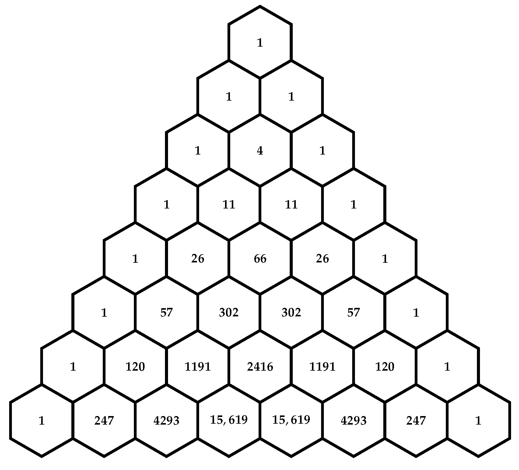
The coefficients of each of these polynomials turn out to be the famous Eulerian coefficients that are the coefficients of an Eulerian polynomial. In fact, here are some known facts about these coefficients $A(n,m)$ and for Eulerian polynomials, $A_n\left(t\right)$ from [5,6,7,8]. These are well-known identities that we recall for the benefit of the reader.

•  

  $$A(1,0)=0,A(1,0)=1,\mathrm{and}A(m,n)=0,\mathrm{for}\mathrm{all}m\ge n$$

  For all other values of n and m,

  $${\displaystyle A(n,m)=\sum _{k=0}^{m+1}{(-1)}^k\left(\genfrac{}{}{0pt}{}{n+1}{k}\right){(m+1-k)}^n}.$$
•  

  $$\sum _{k=1}^N{k}^n=\sum _{m=0}^{n-1}A(n,m)\left(\genfrac{}{}{0pt}{}{N+1+m}{n+1}\right)$$
• (Worpitzky’s identity) [9]

  $$x^n=\sum _{m=0}^{n-1}A(n,m)\left(\genfrac{}{}{0pt}{}{x+m}{n}\right)$$

  $$\sum _{m=0}^{n-1}A(n,m)=n!\mathrm{for}n\ge 1$$
• Similar to binomial coefficients, there is a recursive formula to compute the Eulerian coefficients for appropriate values of m and n.

  $$A(n,m)=(n-m)A(n-1,m-1)+(m+1)A(n-1,m)$$

  $$A_n\left(t\right)=\sum _{k=0}^{n-1}A(n,k)t^k$$

  $$A_0\left(t\right)=1$$

We illustrate Eulerian numbers in a triangle, shown in Figure 1 below.

In the next theorem, we show that the coefficient of $x^n$ in $\frac{G_k\left(x\right)}{(1-x)}$ is nothing but ${\left(P_{k}a\right)}_{\overline{n\hspace{.2em}|}i}$.

Theorem 1.

The present value of an n-year polynomial immediate annuity given by ${\left(P_{k}a\right)}_{\overline{n\hspace{.2em}|}i}$ is the coefficient of $x^n$ in $\frac{G_k\left(x\right)}{(1-x)}$ where $G_k\left(x\right)$ is the generating function for the infinite sequence $\{1^{k}v,2^k{v}^2,3^k{v}^3,\dots \}$.

Proof. 

It can be shown using induction that $G_k\left(x\right)=\frac{v{A}_k\left(vx\right)}{{(1-vx)}^{(k+1)}}$. Recall that we are looking for the coefficient $\left(P_{k}a\right)\overline{n\hspace{.2em}|}i$, which is equal to the coefficient of $x^n$ in

$$\frac{G_k\left(x\right)}{(1-x)}=\left(\frac{v{A}_k\left(vx\right)}{{(1-vx)}^{(k+1)}(1-x)}\right).$$

Euler proved in [5] that

$$\frac{A\left(vx\right)}{{(1-vx)}^{(k+1)}}=\sum _{m=0}^{\infty }{\left(vx\right)}^m{(m+1)}^k.$$

Therefore,

$$\begin{array}{cc}\hfill \frac{vA\left(vx\right)}{{(1-vx)}^{(k+1)}(1-x)}& =\frac{v}{(1-x)}\sum _{m=0}^{\infty }{\left(vx\right)}^m{(m+1)}^k\hfill \\ \hfill & =\left(\sum _{l=0}^{\infty }1x^l\right)\left(\sum _{m=0}^{\infty }{v}^{m+1}{(m+1)}^k{x}^m\right)\hfill \\ \hfill & =\left(\sum _{l=0}^{\infty }{a}_n{x}^l\right)\left(\sum _{m=0}^{\infty }{b}_n{x}^m\right),\hfill \end{array}$$

where $a_l=1$ for all l and $b_m=v^{m+1}{(m+1)}^k$ for all k.

The coefficient of $x^n$ is therefore

$$\begin{array}{cc}\hfill \sum _{j=0}^n{b}_j{a}_{n-j}& =\sum _{j=0}^n{v}^{(j+1)}{(j+1)}^k\hfill \\ \hfill & =\sum _{j=1}^{n+1}{v}^j{j}^k\hfill \\ \hfill & =\left(P_{k}a\right)\overline{n\hspace{.2em}|}i.\hfill \end{array}$$

□

We state and prove the main theorem in the section next.

We recall a lemma from generating functions, which can be easily proven using induction. This lemma will be useful in proving Theorem 2 below:

Lemma 1.

If $a,b\in \mathbb{N}$ and $b>a\ge 0$, then for any $n\ge a$, the coefficient of $x^n$ in

$$\frac{c{x}^a}{{(1-\alpha x)}^b}$$

is

$$c\left(\genfrac{}{}{0pt}{}{n-a+b-1}{b-1}\right){\alpha }^{n-a}.$$

Theorem 2.

Let $A(k,l)$ denote the Eulerian coefficient and $A_k\left(v\right)$ be the Eulerian polynomial evaluated at $v=\frac{1}{1+i}$, where i is the annual effective interest rate. Then, the present value of an n-year polynomial immediate annuity with a payment pattern of $\{1^k,2^k,3^k,\dots ,n^k\}$ is given by the following:

$${\left(P_{k}a\right)}_{\overline{n\hspace{.2em}|}i}=\sum _{j=0}^k{F}_j\left(\genfrac{}{}{0pt}{}{n-j+k}{k}\right)v^{n-j}+B,$$

where

$$\begin{array}{cc}\hfill F_j& =-B\sum _{l-0}^j{(-1)}^l\left(\genfrac{}{}{0pt}{}{k+1}{l}\right)v^l+\sum _{l=0}^{j}A(k,l)v^{(l+1)},j=1,\dots ,k,\hfill \\ \hfill B& =\frac{v{A}_k\left(v\right)}{{(1-v)}^{(k+1)}}.\hfill \end{array}$$

Remark 1.

$F_j^{\prime }s$ and B can also be written as

$$\begin{array}{cc}\hfill B& =\frac{v{A}_k\left(v\right)}{{(1-v)}^{(k+1)}},\hfill \\ \hfill F_j& =B\sum _{l=j+1}^{k+1}\left(\genfrac{}{}{0pt}{}{k+1}{l}\right){(-1)}^l{v}^l-\sum _{l=j+1}^{k}A(k,l)v^{(l+1)},j=1,\dots ,k-1,\hfill \\ \hfill F_k& ={(-1)}^{(k+1)}{v}^{(k+1)}B.\hfill \end{array}$$

Proof. 

Using induction, it can be shown that, in general,

$$G_k\left(x\right)=\frac{v}{{(1-vx)}^{(k+1)}}{A}_k\left(vx\right),\mathrm{where}{A}_k\left(vx\right)\mathrm{is}\mathrm{defined}\mathrm{as}\mathrm{above}.$$

We use partial fractions to produce a new way to derive a formula for the coefficient. The main motivation for the partial fractions approach is that we can use Lemma 1 directly to equate the coefficient of like powers $x^n$ on both sides to obtain the result of this theorem.

Using partial fractions, we seek $F_j$ for $j=0,\dots ,k$ and B such that

$$\left(\frac{v{A}_k\left(vx\right)}{{(1-vx)}^{(k+1)}(1-x)}\right)=\frac{{\sum }_{j=0}^k{F}_j{x}^i}{{(1-vx)}^{(k+1)}}+\frac{B}{(1-x)}.$$

We find a common denominator on the right-hand side and then set the numerators equal to each other. Thus, we find constants $F_j$ for $j=0,\dots ,k$ and B such that

$$\begin{array}{cc}\hfill & \left[\sum _{j=0}^k{F}_j{x}^j\right](1-x)+B{(1-vx)}^{(k+1)}=v{A}_k\left(vx\right).\hfill \end{array}$$

(1)

For $x=1$, we have

$$B{(1-v)}^{(k+1)}=v{A}_k\left(v\right),$$

or

$$B=\frac{v{A}_k\left(v\right)}{{(1-v)}^{(k+1)}}=\frac{v{\sum }_{l=0}^{k-1}A(k,l)v^l}{{(1-v)}^{(k+1)}}.$$

Moving on to $F_j$, for $j=0,\dots ,k$, distribute $(1-x)$ into the summation, and expanding ${(1-vx)}^{(k+1)}$ in (1) above, we obtain

$$\sum _{j=0}^k{F}_j{x}^j-\sum _{j=0}^k{F}_j{x}^{(j+1)}+B\sum _{j=0}^{k+1}\left(\genfrac{}{}{0pt}{}{k+1}{j}\right){\left(vx\right)}^j{(-1)}^j=v\sum _{j=0}^{k-1}A(k,j){\left(vx\right)}^j.$$

Now, we separate the $j=0$ term out from the sum and collect like terms to obtain

$$\begin{array}{cc}\hfill & (F_0+B)+\sum _{j=1}^k(F_j-F_{j-1}+B\left(\genfrac{}{}{0pt}{}{k+1}{j}\right){(-1)}^j{v}^j)x^j+(-F_k+B{v}^{(k+1)}{(-1)}^{(k+1)})x^{(k+1)}\hfill \\ \hfill & =v\sum _{j=0}^{k-1}A(k,j){\left(vx\right)}^j.\hfill \end{array}$$

Thus, when $x=0$, we have

$$F_0+B=vA(k,0),$$

or

$$F_0=-B+vA(k,0).$$

Equating the powers of $x^1$ on both sides of (2), we have:

$$F_1-F_0+{(-1)}^{1}B\left(\genfrac{}{}{0pt}{}{k+1}{1}\right)v^1=v^{2}A(k,1)$$

so,

$$\begin{array}{cc}\hfill F_1& =-B-B\left(\genfrac{}{}{0pt}{}{k+1}{1}\right)v^1{(-1)}^1+vA(k,0)+v^{2}A(k,1)\hfill \\ \hfill & =-B\sum _{l=0}^1{(-1)}^l\left(\genfrac{}{}{0pt}{}{k+1}{l}\right)v^l+\sum _{l=0}^1{v}^{(j+1)}A(k,l).\hfill \end{array}$$

A pattern begins to emerge. Equating coefficients of $x^2$ in (2), we have

$$F_2-F_1+B\left(\genfrac{}{}{0pt}{}{k+1}{1}\right){(-1)}^2{v}^2=v^{3}A(k,2),$$

so,

$$\begin{array}{cc}\hfill F_2& =-F_1-B\left(\genfrac{}{}{0pt}{}{k+1}{2}\right){(-1)}^2{v}^2+v^{3}A(k,2)\hfill \\ \hfill & =-B\sum _{l=0}^1\left(\genfrac{}{}{0pt}{}{k+1}{l}\right){(-1)}^l{v}^l+\sum _{l=0}^1{v}^{j}A(k,l)-B\left(\genfrac{}{}{0pt}{}{k+1}{l}\right)+{(-1)}^2{v}^2\hfill \\ \hfill & =-B\sum _{l=0}^2\left(\genfrac{}{}{0pt}{}{k+1}{l}\right){(-1)}^l{v}^l+\sum _{l=0}^{2}vA{(k,l)}^{(j+1)}.\hfill \end{array}$$

In general, by equating the powers of $x^j$ on both sides, we obtain

$$F_j=-B\sum _{l=0}^j\left(\genfrac{}{}{0pt}{}{k+1}{l}\right){(-1)}^l{v}^l+\sum _{l=0}^{j}vA{(k,l)}^{(j+1)},\mathrm{for}j=0,1,2,\dots ,k.$$

We could also obtain these coefficients by working backwards from k to obtain the following:

$$\begin{array}{cc}\hfill B& =\frac{v{A}_k\left(v\right)}{{(1-v)}^{(k+1)}},\hfill \\ \hfill F_j& =B\sum _{l=j+1}^{k+1}\left(\genfrac{}{}{0pt}{}{k+1}{l}\right){(-1)}^l{v}^l-\sum _{l=j+1}^{k}A(k,l)v^{(l+1)},j=1,\dots ,k-1,\hfill \\ \hfill F_k& ={(-1)}^{(k+1)}{v}^{(k+1)}B.\hfill \end{array}$$

The proof follows by applying Lemma 1 and computing the coefficient of $x^n$ in

$$\left(\frac{v{A}_k\left(vx\right)}{{(1-vx)}^{(k+1)}(1-x)}\right)=\frac{{\sum }_{j=0}^k{F}_j{x}^i}{{(1-vx)}^{(k+1)}}+\frac{B}{(1-x)}.$$

This proves the theorem. □

3. Method 2: Using Geometric Series

In this section, we show an alternate method to obtain a closed-form expression for ${\left(P_{k}a\right)}_{\overline{n\hspace{.2em}|}i}$. The final result, however, was already derived by Euler in [5], albeit using a combinatorial approach.

Theorem 3.

Let $A(k,l)$ denote the Eulerian coefficient and $A_k\left(v\right)$ be the Eulerian polynomial evaluated at $v=\frac{1}{1+i}$, where i is the annual effective interest rate. Then, the present value of an n-year polynomial immediate annuity with a payment pattern of $\{1^k,2^k,3^k,\dots ,n^k\}$ is given by the following two equivalent expressions:

$$\begin{array}{c}\hfill {\left(P_{k}a\right)}_{\overline{n\hspace{.2em}|}i}=-v^{(n+1)}\sum _{l=0}^k\left(\begin{array}{c}k\\ l\end{array}\right)\frac{A_l\left(v\right)n^{(k-l)}}{{(1-v)}^{(l+1)}}+\frac{v{A}_k\left(v\right)}{{(1+v)}^{(k+1)}},\end{array}$$

(2)

or

$${\left(P_{k}a\right)}_{\overline{n\hspace{.2em}|}i}=\sum _{l=0}^k\left(\begin{array}{c}k\\ l\end{array}\right){(-1)}^{(k-l)}{n}^l{v}^{n+1}\frac{A_{k-l}\left(v\right)}{{(v-1)}^{(k-l+1)}}-{(-1)}^k\frac{v{A}_k\left(v\right)}{{(v-1)}^{(k+1)}}.$$

Remark 2.

At the outset, we want to reiterate that the result above was proven by Euler in [5]. We are merely showing an alternate derivation method to show the same result here.

Proof. 

Let $v=e^{-\delta }$ and consider

$$\begin{array}{cc}\hfill F\left(x\right)=v{e}^x+v^2{e}^{2x}+v^3{e}^{3x}+\cdots +v^n{e}^{nx}& =\frac{{\left(v{e}^x\right)}^{(n+1)}-v{e}^x}{(v{e}^x-1)}\hfill \\ \hfill & =\frac{e^{(x-\delta )(n+1)}-e^{x-\delta }}{e^{x-\delta }-1}\hfill \\ \hfill & =\frac{e^{(x-\delta )}·\{e^{n(x-\delta )}-1\}}{e^{x-\delta }-1}.\hfill \end{array}$$

Note that

$$\begin{array}{cc}\hfill F\left(0\right)& =v+v^2+\cdots +v^n=a_{\overline{n\hspace{.2em}|}i}\hfill \\ \hfill F^{\prime }\left(0\right)& =v+2v^2+3v^3+\cdots +n{v}^n={\left(P_{1}a\right)}_{\overline{n\hspace{.2em}|}i}\hfill \\ \hfill F^{\prime \prime }\left(0\right)& =v+2^2{v}^2+3^2{v}^3+\cdots +n^2{v}^n={\left(P_{2}a\right)}_{\overline{n\hspace{.2em}|}i}\hfill \\ \hfill F^{\prime \prime \prime }\left(0\right)& =v+2^3{v}^2+3^3{v}^3+\cdots +n^3{v}^n={\left(P_{3}a\right)}_{\overline{n\hspace{.2em}|}}i\hfill \\ \hfill ⋮\\ \hfill F^{\left(k\right)}\left(0\right)& ={\left(P_{k}a\right)}_{\overline{n\hspace{.2em}|}i}.\hfill \end{array}$$

Therefore, we can conclude that the Taylor series expansion of the right-hand side of $G\left(x\right)$ above is

$$\left(a_{\overline{n\hspace{.2em}|}i}\right)+{\left(P_{1}a\right)}_{\overline{n\hspace{.2em}|}i}\frac{x}{1!}+{\left(P_{2}a\right)}_{\overline{n\hspace{.2em}|}i}\frac{x^2}{2!}+\cdots +{\left(P_{k}a\right)}_{\overline{n\hspace{.2em}|}i}\frac{x^k}{k!}+\cdots .$$

We now concentrate on the right-hand side of $F\left(x\right)$, namely

$$\frac{e^{(x-\delta )}·\{e^{n(x-\delta )}-1\}}{e^{x-\delta }-1}.$$

Let $A_k\left(e^{x-\delta }\right)$ be the Euler polynomial evaluated at $e^{x-\delta }$. We can now derive the following. We define the function $H\left(x\right)$ as follows:

$$H\left(x\right)=\frac{e^{(x-\delta )}}{e^{x-\delta }-1}=1+\frac{1}{e^{x-\delta }-1},$$

Thus,

$$\begin{array}{cc}\hfill H^{\prime }\left(x\right)& =-\frac{e^{x-\delta }}{{(e^{x-\delta }-1)}^2},\hfill \\ \hfill H^{\prime \prime }\left(x\right)& =\frac{e^{x-\delta }\{e^{x-\delta }+1\}}{{(e^{x-\delta }-1)}^3},\hfill \\ \hfill H^{\prime \prime \prime }\left(x\right)& =-\frac{e^{x-\delta }\{e^{2(x-\delta )}+4e^{x-\delta }+1\}}{{(e^{x-\delta }-1)}^4}=-\frac{e^{x-\delta }{A}_3\left(e^{x-\delta }\right)}{{(e^{x-\delta }-1)}^4},\hfill \\ \hfill H^{\left(4\right)}\left(x\right)& =\frac{e^{x-\delta }\{e^{3(x-\delta )}+11e^{2(x-\delta )}+11e^{x-\delta }+1\}}{{(e^{x-\delta }-1)}^5}=\frac{e^{x-\delta }{A}_4\left(e^{x-\delta }\right)}{{(e^{x-\delta }-1)}^5},\hfill \\ \hfill ⋮\\ \hfill H^{\left(k\right)}\left(x\right)& =\frac{{(-1)}^k{e}^{x-\delta }{A}_k\left(e^{x-\delta }\right)}{{(e^{x-\delta }-1)}^{(k+1)}}.\hfill \end{array}$$

Now, we define $U\left(x\right)=e^{n(x-\delta )}$ so that

$$F\left(x\right)=H\left(x\right)·U\left(x\right).$$

Note that

$$H^{\left(k\right)}\left(x\right)=\frac{{(-1)}^k{e}^{x-\delta }{A}_k\left(e^{x-\delta }\right)}{{(e^{x-\delta }-1)}^{(k+1)}},$$

and

$$U^{\left(k\right)}\left(x\right)=n^k{e}^{n(x-\delta )}-1(k=0),$$

$1(k=l)$ is the indicator function that returns the value of 1 if $k=l$ and 0 otherwise. Therefore, by the Leibniz formula for the derivative of products,

$$\begin{array}{cc}\hfill F^{\left(k\right)}\left(x\right)& =\sum _{l=0}^k\left(\begin{array}{c}k\\ l\end{array}\right)H^{\left(l\right)}\left(x\right)U^{(k-l)}\left(x\right)\hfill \\ \hfill & =\sum _{l=0}^k\left(\begin{array}{c}k\\ l\end{array}\right)\frac{{(-1)}^k{e}^{(x-\delta )}{A}_l(e^{(x-\delta )}}{{(e^{(x-\delta )}-1)}^{(l+1)}}\left[n^{(k-l)}{e}^{(x-\delta )}-1(k=l)\right].\hfill \end{array}$$

Thus,

$$\begin{array}{c}\hfill F^{\left(k\right)}\left(0\right)=-v^{(n+1)}\sum _{l=0}^k\left(\begin{array}{c}k\\ l\end{array}\right)\frac{A_l\left(v\right)n^{(k-l)}}{{(1-v)}^{(l+1)}}+\frac{v{A}_k\left(v\right)}{{(1+v)}^{(k+1)}}.\end{array}$$

(3)

If we write it the other way, we have the following:

$$\begin{array}{cc}\hfill F^{\left(k\right)}\left(x\right)& =\sum _{l=0}^k\left(\begin{array}{c}k\\ l\end{array}\right)U^{\left(l\right)}\left(x\right)H^{(k-l)}\left(x\right)\hfill \\ \hfill & =\sum _{l=0}^k\left(\begin{array}{c}k\\ l\end{array}\right)\left[n^l{e}^{n(x-\delta )}-1(k=0)\right]·\frac{{(-1)}^{(k-l)}{e}^{(x-\delta )}{A}_{k-l}\left(e^{x-\delta }\right)}{{(e^{(x-\delta )}-1)}^{(k-l+1)}}.\hfill \end{array}$$

Thus,

$$F^{\left(k\right)}\left(0\right)=\sum _{l=0}^k\left(\begin{array}{c}k\\ l\end{array}\right){(-1)}^{(k-l)}{n}^l{v}^{n+1}\frac{A_{k-l}\left(v\right)}{{(v-1)}^{(k-l+1)}}-{(-1)}^k\frac{v{A}_k\left(v\right)}{{(v-1)}^{(k+1)}}.$$

This proves the theorem. □

4. Continuous Polynomial Annuities

In this section, we turn our attention to continuous polynomial annuities where the payment rate is $t^k$ USD per unit time, as illustrated in Figure 2 below. Here, we use the equivalence $v=e^{-\delta }$ for continuous annuities.

In this case, the payment for a small interval of time $dt$ is equal to $t^{k}dt$. Thus, the present value of $t^{k}dt$ at time $t=0$ is $\left(t^{k}dt\right)v^t$. There are infinitely many such pieces of time $\left(dt\right)$ We introduce notation that signifies a continuous increase and compounding over time.

$$\left(\overline{P_k}\overline{a}\right)\overline{n\hspace{.2em}|}i={\int }_0^n{t}^k{e}^{-\delta t}dt$$

Theorem 4.

The present value of a continuous n-year polynomial immediate annuity, denoted by ${\left({\overline{P}}_k\overline{a}\right)}_{\overline{n\hspace{.2em}|}i}$, with a payment rate of $t^k$ USD per unit time is given by the following:

$$\begin{array}{cc}\hfill {\left({\overline{P}}_k\overline{a}\right)}_{\overline{n\hspace{.2em}|}i}& ={\int }_0^n{t}^k{e}^{-\delta t}dt\hfill \\ \hfill & =-\frac{e^{-\delta n}}{\delta }\sum _{l=0}^{(k-1)}\frac{k^l}{{\delta }^l}{n}^{(k-l)}+\frac{k!}{{\delta }^k}\left(\frac{1-e^{-\delta n}}{\delta }\right)\hfill \\ \hfill & =\frac{1}{{\delta }^{(k+1)}}\gamma ((k-1),n\delta ),\hfill \end{array}$$

where $\gamma (s,x)={\int }_0^x{t}^{(s-1)}{e}^{-t}dt$, the lower incomplete gamma function.

Proof. 

We develop a recursion using the technique of integration by parts. Thus,

$$\begin{array}{cc}\hfill {\left({\overline{P}}_k\overline{a}\right)}_{\overline{n\hspace{.2em}|}i}& ={\int }_0^n{t}^k{e}^{-\delta t}dt\hfill \\ \hfill & =\frac{-t^k{e}^{-\delta n}}{\delta }{|}_{t=0}^{t=n}+\frac{k}{\delta }{\int }_0^n{t}^{(k-1}{e}^{-\delta t}dt\hfill \\ \hfill & =-\frac{n^k{e}^{-\delta n}}{\delta }+\frac{k}{\delta }{\left({\overline{P}}_{k-1}\overline{a}\right)}_{\overline{n\hspace{.2em}|}i}\hfill \\ \hfill & =-\frac{n^k{e}^{-\delta n}}{\delta }+\frac{k}{\delta }\left[\frac{-n^{(k-1)}{e}^{-\delta n}}{\delta }+\frac{(k-1)}{\delta }{\left({\overline{P}}_{k-2}\overline{a}\right)}_{\overline{n\hspace{.2em}|}i}\right]\hfill \\ \hfill & =-\frac{e^{-\delta n}}{\delta }\left\{n^k+\frac{k}{\delta }{n}^{(k-1)}\right\}+\frac{k(k-1)}{{\delta }^2}\left\{{\overline{P}}_{k-2}\overline{a}{)}_{\overline{n\hspace{.2em}|}i}\right\}\hfill \\ \hfill & =-\frac{e^{-\delta n}}{\delta }\left\{n^k+\frac{k}{\delta }{n}^{(k-1)}\right\}+\frac{k(k-1)}{{\delta }^2}\left\{\frac{-n^{(k-2)}{e}^{-\delta n}}{\delta }+\frac{(k-2)}{\delta }{\left({\overline{P}}_{k-3}\overline{a}\right)}_{\overline{n\hspace{.2em}|}i}\right\}\hfill \\ \hfill & =-\frac{e^{-\delta n}}{\delta }\sum _{l=0}^2\frac{k^l}{{\delta }^l}{n}^{(k-l)}+\frac{k(k-1)(k-2)}{{\delta }^3}{\left({\overline{P}}_{k-3}\overline{a}\right)}_{\overline{n\hspace{.2em}|}i}\hfill \\ \hfill & =-\frac{e^{-\delta n}}{\delta }\sum _{l=0}^2\frac{k^l}{{\delta }^l}{n}^{(k-l)}+\frac{k^{\underline{3}}}{{\delta }^3}{\left({\overline{P}}_{k-3}\overline{a}\right)}_{\overline{n\hspace{.2em}|}i},\mathrm{where}{k}^{\underline{3}}=k(k-1)(k-2)\hfill \\ \hfill & =-\frac{e^{-\delta n}}{\delta }\sum _{l=0}^3\frac{k^l}{{\delta }^l}{n}^{(k-l)}+\frac{k^{\underline{4}}}{{\delta }^4}{\left({\overline{P}}_{k-4}\overline{a}\right)}_{\overline{n\hspace{.2em}|}i}\hfill \\ \hfill & =-\frac{e^{-\delta n}}{\delta }\sum _{l=0}^j\frac{k^l}{{\delta }^l}{n}^{(k-l)}+\frac{k^{\underline{(j+1)}}}{{\delta }^{(j+1)}}{\left({\overline{P}}_{k-(j+1)}\overline{a}\right)}_{\overline{n\hspace{.2em}|}i}.\hfill \end{array}$$

Now, when $j=k-1$, we have

$$\begin{array}{cc}\hfill {\left({\overline{P}}_k\overline{a}\right)}_{\overline{n\hspace{.2em}|}i}& =-\frac{e^{-\delta n}}{\delta }\sum _{l=0}^{(k-1)}\frac{k^l}{{\delta }^l}{n}^{(k-l)}+\frac{k^{\underline{k}}}{{\delta }^k}{\left({\overline{P}}_0\overline{a}\right)}_{\overline{n\hspace{.2em}|}i}\hfill \\ \hfill & =-\frac{e^{-\delta n}}{\delta }\sum _{l=0}^{(k-1)}\frac{k^l}{{\delta }^l}{n}^{(k-l)}+\frac{k!}{{\delta }^k}{\left({\overline{P}}_0\overline{a}\right)}_{\overline{n\hspace{.2em}|}i}.\hfill \end{array}$$

We can summarize this work for continuous annuities as

$$\begin{array}{cc}\hfill {\left({\overline{P}}_0\overline{a}\right)}_{\overline{n\hspace{.2em}|}i}& ={\overline{a}}_{\overline{n\hspace{.2em}|}i}=\frac{1-e^{-\delta n}}{\delta }\hfill \\ \hfill {\left({\overline{P}}_k\overline{a}\right)}_{\overline{n\hspace{.2em}|}i}& =-\frac{e^{-\delta n}}{\delta }\sum _{l=0}^{(k-1)}\frac{k^l}{{\delta }^l}{n}^{(k-l)}+\frac{k!}{{\delta }^k}{\left({\overline{P}}_0\overline{a}\right)}_{\overline{n\hspace{.2em}|}i}\hfill \\ \hfill & =-\frac{e^{-\delta n}}{\delta }\sum _{l=0}^{(k-1)}\frac{k^l}{{\delta }^l}{n}^{(k-l)}+\frac{k!}{{\delta }^k}\left(\frac{1-e^{-\delta n}}{\delta }\right).\hfill \end{array}$$

Note that the integral associated with ${\left({\overline{P}}_k\overline{a}\right)}_{\overline{n\hspace{.2em}|}i}$ is related to the lower incomplete gamma function, which is defined by

$$\gamma (s,x)={\int }_0^x{t}^{(s-1)}{e}^{-t}dt.$$

Indeed, if we let $\delta t=u$ and perform a change of variables, we obtain

$$\begin{array}{cc}\hfill {\left({\overline{P}}_k\overline{a}\right)}_{\overline{n\hspace{.2em}|}i}& ={\int }_0^n{t}^k{e}^{-\delta t}dt\hfill \\ \hfill & ={\int }_0^{n\delta }{\left(\frac{u}{\delta }\right)}^k{e}^{-u}\left(\frac{1}{\delta }du\right)\hfill \\ \hfill & =\frac{1}{{\delta }^{(k+1)}}{\int }_0^{n\delta }{u}^{(k-1+1)}{e}^{-u}du\hfill \\ \hfill & =\frac{1}{{\delta }^{(k+1)}}\gamma ((k-1),n\delta ).\hfill \end{array}$$

This proves the theorem. □

5. m-Monthly Payments

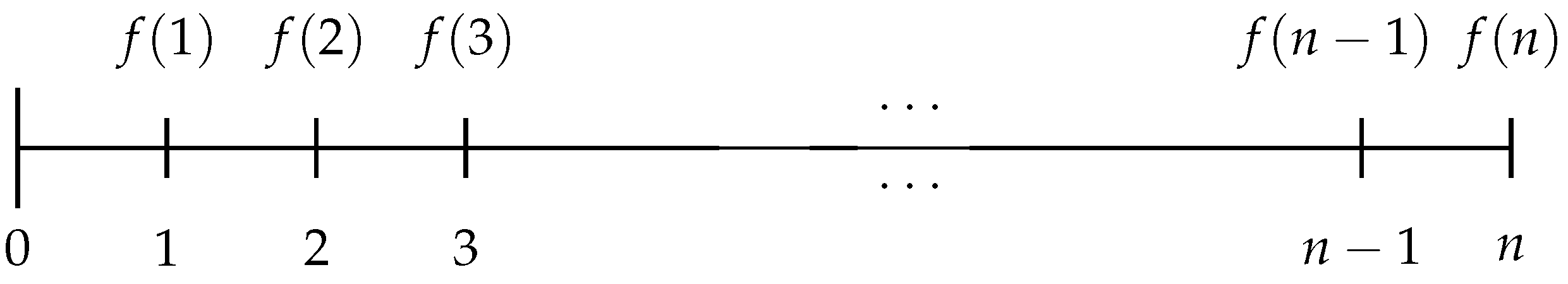
In this section, we derive an expression for the present value of an n-year polynomial immediate annuity that is based on m-monthly payments.

Define ${\left(P_k^{\left(m\right)}{a}^{\left(m\right)}\right)}_{\overline{n\hspace{.2em}|}i}$ as the monthly payment, where the superscript indicates a payment frequency of m times per year.

In this situation, as shown in Figure 3 below, the payments need to be divided by $m^{(k+1)}$, as illustrated in the figure. This is to mimic the Riemann approximation [10] of the total amount of money paid at a rate of $t^k$ USD per unit time from $t=0$ to $t=n$.

Note that this is connected to the continuous case, $t^k$ USD per unit time, so that the total amount of money in n years will be

$${\int }_0^n{t}^{k}dt.$$

The Riemann sum [10] approximates the total money, which is a definite integral from $t=0$ to $t=n$, as the sum of the areas of rectangles, each of which represents an equivalent discrete approximate payment. In the limit that m goes to ∞, the approximation is exact.

$${\int }_0^n{t}^{k}dt\approx \frac{1}{m}\sum _{l=1}^{nm}{\left(\frac{l}{m}\right)}^k=\frac{1^k}{m^{(k+1)}}+\frac{2^k}{m^{(k+1)}}+\cdots +\frac{{\left(nm\right)}^k}{m^{(k+1)}}.$$

The individual terms are the USD amounts so that in the limiting case, the total money is the same.

Note that we use the right-hand endpoint to make this approximation, where the payment occurs at the end of each interval of time. That is,

$$\underset{m\to \infty }{lim}\frac{1}{m}\sum _{l=1}^{nm}{\left(\frac{l}{m}\right)}^k={\int }_0^n{t}^{k}dt.$$

Theorem 5.

Let $A(k,l)$ denote the Eulerian coefficient and $A_k\left(\widehat{v}\right)$ be the Eulerian polynomial evaluated at $\widehat{v}=\frac{1}{1+\widehat{i}}$, where $\widehat{i}=\frac{i^{\left(m\right)}}{m}$. Then, the present value of an n-year m-monthly polynomial immediate annuity, denoted by ${\left(P_k^{\left(m\right)}{a}^{\left(m\right)}\right)}_{\overline{n\hspace{.2em}|}i}$ with a payment pattern of $\left\{\frac{1^k}{m^{k+1}},\frac{2^k}{m^{k+1}},\frac{3^k}{m^{k+1}},\dots ,\frac{{\left(nm\right)}^k}{m^{k+1}}\right\}$, is given by the following two equivalent expressions:

$$\begin{array}{cc}\hfill \left(P_k^{\left(m\right)}{a}^{\left(m\right)}\right)\overline{n\hspace{.2em}|}i& =\frac{1}{m^{(k+1)}}\left\{-{\widehat{v}}^{(nm+1)}\sum _{l=0}^k\left(\genfrac{}{}{0pt}{}{k}{l}\right)\frac{A_l\left(\widehat{v}{\left(nm\right)}^{(k-l)}\right)}{{(1-\widehat{v})}^{(l+1)}}+\frac{\widehat{v}{A}_k\left(\widehat{v}\right)}{{(1-\widehat{v})}^{(k+1)}}\right\}\hfill \\ \hfill & =\frac{1}{m^{(k+1)}}\left\{{\widehat{v}}^{(nm+1)}\sum _{l=0}^k{(-1)}^{(k-l)}{\left(nm\right)}^l\frac{A_{k-l}\left(\widehat{v}\right)}{{(\widehat{v}-1)}^{(k-l+1)}}-\frac{{(-1)}^k\widehat{v}{A}_k\left(\widehat{v}\right)}{{(\widehat{v}-1)}^{(k+1)}}\right\},\mathrm{and}\hfill \\ \hfill \left(P_k^{\left(m\right)}{a}^{\left(m\right)}\right)\overline{n\hspace{.2em}|}i& =\frac{1}{m^{(k+1)}}\left\{\sum _{j=0}^k{\widehat{F}}_j\left(\genfrac{}{}{0pt}{}{nm-j+k}{k}\right){\widehat{v}}^{(nm-j)}+\frac{\widehat{v}{A}_k\left(\widehat{v}\right)}{{(1-\widehat{v})}^{(k+1)}}\right\},\hfill \end{array}$$

where

$$\begin{array}{cc}\hfill {\widehat{F}}_j& =-\widehat{B}\sum _{l=0}^j{(-1)}^l\left(\genfrac{}{}{0pt}{}{k+1}{l}\right){\widehat{v}}^l+\sum _{l=0}^{j}A(k,l){\widehat{v}}^{(l+1)},j=1,\dots ,k-1,\hfill \\ \hfill {\widehat{F}}_k& ={(-1)}^{(k+1)}{\widehat{v}}^{(k+1)}\widehat{B},\hfill \\ \hfill \widehat{B}& =\frac{\widehat{v}{A}_k\left(\widehat{v}\right)}{{(1-\widehat{v})}^{(k+1)}}.\hfill \end{array}$$

Proof. 

If we first factor out $\frac{1}{m^{(k+1)}}$ from all payments, then we have

$$\frac{1}{m^{(k+1)}}·\{1^k,2^k,\dots ,{\left(nm\right)}^k\}$$

as the payment sequence. There are $\left(nm\right)$ periods with periodic interest rate $\frac{i^m}{m}$. Thus,

$${\left(P_k^{\left(m\right)}{a}^{\left(m\right)}\right)}_{\overline{n\hspace{.2em}|}i}=\frac{1}{m^{(k+1)}}·{\left(P_{k}a\right)}_{\overline{nm\hspace{.2em}|}\frac{i^{\left(m\right)}}{m}},$$

and furthermore,

$$\underset{m\to \infty }{lim}{\left(P_k^{\left(m\right)}{a}^{\left(m\right)}\right)}_{\overline{n\hspace{.2em}|}i}={\left({\overline{P}}_k\overline{a}\right)}_{\overline{n\hspace{.2em}|}i}.$$

We now unravel the left- and right-hand sides. We have already shown that

$${\left({\overline{P}}_k\overline{a}\right)}_{\overline{n\hspace{.2em}|}i}=\frac{1}{{\delta }^{(k+1)}}\gamma ((k+1),n\delta ),$$

where $\gamma (s,x)={\int }_0^x{t}^{(s-1)}{e}^{-t}dt$, the lower incomplete gamma function.

Let $\widehat{i}=\frac{i^{\left(m\right)}}{m}$ and $\widehat{v}=\frac{1}{1+\widehat{i}}$. Then, the left-hand side above is calculated using Theorem 3 as follows:

$$\begin{array}{cc}\hfill \left(P_k^{\left(m\right)}{a}^{\left(m\right)}\right)\overline{n\hspace{.2em}|}i& =\frac{1}{m^{(k+1)}}{\left(P_{k}a\right)}_{\overline{nm\hspace{.2em}|}\frac{i^{\left(m\right)}}{m}}\hfill \\ \hfill & =\frac{1}{m^{(k+1)}}\left\{-{\widehat{v}}^{(nm+1)}\sum _{l=0}^k\left(\genfrac{}{}{0pt}{}{k}{l}\right)\frac{A_l\left(\widehat{v}{\left(nm\right)}^{(k-l)}\right)}{{(1-\widehat{v})}^{(l+1)}}+\frac{\widehat{v}{A}_k\left(\widehat{v}\right)}{{(1-\widehat{v})}^{(k+1)}}\right\}\hfill \\ \hfill & =\frac{1}{m^{(k+1)}}\left\{{\widehat{v}}^{(nm+1)}\sum _{l=0}^k{(-1)}^{(k-l)}{\left(nm\right)}^l\frac{A_{k-l}\left(\widehat{v}\right)}{{(\widehat{v}-1)}^{(k-l+1)}}-\frac{{(-1)}^k\widehat{v}{A}_k\left(\widehat{v}\right)}{{(\widehat{v}-1)}^{(k+1)}}\right\}.\hfill \end{array}$$

Using Theorem 2, we also have

$${\left(P_k^{\left(m\right)}{a}^{\left(m\right)}\right)}_{\overline{n\hspace{.2em}|}i}=\frac{1}{m^{(k+1)}}\left\{\sum _{j=0}^k{\widehat{F}}_j\left(\genfrac{}{}{0pt}{}{nm-j+k}{k}\right){\widehat{v}}^{(nm-j)}+\frac{\widehat{v}{A}_k\left(\widehat{v}\right)}{{(1-\widehat{v})}^{(k+1)}}\right\},$$

where

$$\begin{array}{cc}\hfill {\widehat{F}}_j& =-\widehat{B}\sum _{l-0}^j{(-1)}^l\left(\genfrac{}{}{0pt}{}{k+1}{l}\right){\widehat{v}}^l+\sum _{l=0}^{j}A(k,l){\widehat{v}}^{(l+1)},j=1,\dots ,k-1,\hfill \\ \hfill {\widehat{F}}_k& ={(-1)}^{(k+1)}{\widehat{v}}^{(k+1)}\widehat{B},\hfill \\ \hfill \widehat{B}& =\frac{\widehat{v}{A}_k\left(\widehat{v}\right)}{{(1-\widehat{v})}^{(k+1)}}.\hfill \end{array}$$

This proves the theorem □

Now, using the expressions from Method 1 and Method 2 from earlier in the paper, we compute the limit as m goes to infinity for both expressions. As m, the number of payments per year $\to \infty$, we have that

$$\underset{m\to \infty }{lim}{\left(P_k^{\left(m\right)}{a}^{\left(m\right)}\right)}_{\overline{n\hspace{.2em}|}i}={\left({\overline{P}}_k\overline{a}\right)}_{\overline{n\hspace{.2em}|}i}$$

or in other words, the payments become continuous.

$$\begin{array}{cc}\hfill \underset{m\to \infty }{lim}{\left(P_k^{\left(m\right)}{a}^{\left(m\right)}\right)}_{\overline{n\hspace{.2em}|}i}& =\underset{m\to \infty }{lim}\frac{1}{m^{(k+1)}}\left\{-{\widehat{v}}^{(nm+1)}\sum _{l=0}^k\left(\genfrac{}{}{0pt}{}{k}{l}\right)\frac{A_l\left(\widehat{v}{\left(nm\right)}^{(k-l)}\right)}{{(1-\widehat{v})}^{(l+1)}}+\frac{\widehat{v}{A}_k\left(\widehat{v}\right)}{{(1-\widehat{v})}^{(k+1)}}\right\}\hfill \\ \hfill & =\underset{m\to \infty }{lim}\frac{1}{m^{(k+1)}}\left\{{\widehat{v}}^{(nm+1)}\sum _{l=0}^k{(-1)}^{(k-l)}{\left(nm\right)}^l\frac{A_{k-l}\left(\widehat{v}\right)}{{(\widehat{v}-1)}^{(k-l+1)}}-\frac{{(-1)}^k\widehat{v}{A}_k\left(\widehat{v}\right)}{{(\widehat{v}-1)}^{(k+1)}}\right\}\hfill \\ \hfill & =\underset{m\to \infty }{lim}\frac{1}{m^{(k+1)}}\left\{\sum _{j=0}^k{\widehat{F}}_j\left(\genfrac{}{}{0pt}{}{nm-j+k}{k}\right){\widehat{v}}^{(nm-j)}+\frac{\widehat{v}{A}_k\left(\widehat{v}\right)}{{(1-\widehat{v})}^{(k+1)}}\right\}\hfill \\ \hfill & ={\left({\overline{P}}_k\overline{a}\right)}_{\overline{n\hspace{.2em}|}i}=\frac{1}{{\delta }^{(k+1)}}\gamma ((k+1),n\delta ),\hfill \end{array}$$

where

$$\begin{array}{cc}\hfill {\widehat{F}}_j& =-\widehat{B}\sum _{l-0}^j{(-1)}^l\left(\genfrac{}{}{0pt}{}{k+1}{l}\right){\widehat{v}}^l+\sum _{l=0}^{j}A(k,l){\widehat{v}}^{(l+1)},j=1,\dots ,k-1,\hfill \\ \hfill {\widehat{F}}_k& ={(-1)}^{(k+1)}{\widehat{v}}^{(k+1)}\widehat{B},\hfill \\ \hfill \widehat{B}& =\frac{\widehat{v}{A}_k\left(\widehat{v}\right)}{{(1-\widehat{v})}^{(k+1)}}.\hfill \end{array}$$

We can input $\widehat{i}=\frac{i^{\left(m\right)}}{m}={(1+i)}^{1/m}-1$, $\delta =ln(1+i)$, and $\widehat{v}=\frac{1}{{(1+i)}^{1/m}}$ in the limits above if we want explicit dependence on m.

This limit relates the Eulerian polynomials to the lower incomplete gamma function. We state this relationship in the form of the following theorem.

Theorem 6.

$$\begin{array}{cc}\hfill \frac{1}{{\delta }^{(k+1)}}\gamma ((k+1),n\delta )& =\underset{m\to \infty }{lim}\frac{1}{m^{(k+1)}}\left\{-{\widehat{v}}^{(nm+1)}\sum _{l=0}^k\left(\genfrac{}{}{0pt}{}{k}{l}\right)\frac{A_l\left(\widehat{v}{\left(nm\right)}^{(k-l)}\right)}{{(1-\widehat{v})}^{(l+1)}}+\frac{\widehat{v}{A}_k\left(\widehat{v}\right)}{{(1-\widehat{v})}^{(k+1)}}\right\}\hfill \\ \hfill & =\underset{m\to \infty }{lim}\frac{1}{m^{(k+1)}}\left\{{\widehat{v}}^{(nm+1)}\sum _{l=0}^k{(-1)}^{(k-l)}{\left(nm\right)}^l\frac{A_{k-l}\left(\widehat{v}\right)}{{(\widehat{v}-1)}^{(k-l+1)}}-\frac{{(-1)}^k\widehat{v}{A}_k\left(\widehat{v}\right)}{{(\widehat{v}-1)}^{(k+1)}}\right\}\hfill \\ \hfill & =\underset{m\to \infty }{lim}\frac{1}{m^{(k+1)}}\left\{\sum _{j=0}^k{\widehat{F}}_j\left(\genfrac{}{}{0pt}{}{nm-j+k}{k}\right){\widehat{v}}^{(nm-j)}+\frac{\widehat{v}{A}_k\left(\widehat{v}\right)}{{(1-\widehat{v})}^{(k+1)}}\right\},\hfill \end{array}$$

where

$$\begin{array}{cc}\hfill {\widehat{F}}_j& =-\widehat{B}\sum _{l-0}^j{(-1)}^l\left(\genfrac{}{}{0pt}{}{k+1}{l}\right){\widehat{v}}^l+\sum _{l=0}^{j}A(k,l){\widehat{v}}^{(l+1)},j=1,\dots ,k-1,\hfill \\ \hfill {\widehat{F}}_k& ={(-1)}^{(k+1)}{\widehat{v}}^{(k+1)}\widehat{B},\hfill \\ \hfill \widehat{B}& =\frac{\widehat{v}{A}_k\left(\widehat{v}\right)}{{(1-\widehat{v})}^{(k+1)}}.\hfill \end{array}$$

6. Polynomial Perpetuity

In this section, we consider the present value of an annual and m-monthly polynomial immediate perpetuity, denoted by ${\left(P_{k}a\right)}_{\overline{\infty \hspace{.2em}|}i}$ and ${\left(P_k^{\left(m\right)}{a}^{\left(m\right)}\right)}_{\overline{\infty \hspace{.2em}|}i}$ with payment patterns of $\left\{1^k,2^k,3^k,\dots \right\}$ and $\left\{\frac{1^k}{m^{k+1}},\frac{2^k}{m^{k+1}},\frac{3^k}{m^{k+1}},\dots ,\frac{{\left(nm\right)}^k}{m^{k+1}}\right\}$, respectively. We state and prove a theorem to that effect.

Theorem 7.

Let $A(k,l)$ denote the Eulerian coefficient, $A_k\left(\widehat{v}\right)$, and $A_k\left(\widehat{v}\right)$ be the Eulerian polynomial evaluated at $\widehat{v}=\frac{1}{1+\widehat{i}},v=\frac{1}{1+i}$, where $\widehat{i}=\frac{i^{\left(m\right)}}{m}$. Then, the present value of an annual and m-monthly polynomial immediate perpetuity, denoted by ${\left(P_{k}a\right)}_{\overline{\infty \hspace{.2em}|}i}$ and ${\left(P_k^{\left(m\right)}{a}^{\left(m\right)}\right)}_{\overline{\infty \hspace{.2em}|}i}$ with payment patterns of $\left\{1^k,2^k,3^k,\dots \right\}$ and $\left\{\frac{1^k}{m^{k+1}},\frac{2^k}{m^{k+1}},\frac{3^k}{m^{k+1}},\dots ,\frac{{\left(nm\right)}^k}{m^{k+1}}\right\}$, respectively, is given by the following expressions:

$${\left(P_{k}a\right)}_{\overline{\infty \hspace{.2em}|}i}=\frac{v{A}_k\left(v\right)}{{(1-v)}^{(k+1)}};\mathrm{and}{\left(P_k^{\left(m\right)}{a}^{\left(m\right)}\right)}_{\overline{\infty \hspace{.2em}|}i}=\frac{\widehat{v}{A}_k\left(\widehat{v}\right)}{{(1-\widehat{v})}^{(k+1)}}.$$

Proof. 

An explicit expression for ${\left(P_{k}a\right)}_{\overline{\infty \hspace{.2em}|}i}$ can be obtained by taking the limit as $n\to \infty$ in the expression for ${\left(P_{k}a\right)}_{\overline{n\hspace{.2em}|}i}$ in Theorems 2 and 3 and noting that all terms go to zero, except for the following term in both theorems.

$$\begin{array}{cc}\hfill \mathrm{Polynomial}\mathrm{Perpetuity}& ={\left(P_{k}a\right)}_{\overline{\infty \hspace{.2em}|}i}\hfill \\ \hfill & =\underset{n\to \infty }{lim}{\left(P_{k}a\right)}_{\overline{n\hspace{.2em}|}i}\hfill \\ \hfill & =\frac{v{A}_k\left(v\right)}{{(1-v)}^{(k+1)}}\hfill \end{array}$$

In a similar way, we can derive the m-monthly perpetuity ${\left(P_k^{\left(m\right)}{a}^{\left(m\right)}\right)}_{\overline{\infty \hspace{.2em}|}i}$ by letting $n\to \infty$ in the expression for ${\left(P_k^{\left(m\right)}{a}^{\left(m\right)}\right)}_{\overline{n\hspace{.2em}|}i}$ in Theorem 5 and, once again, noting that all terms go to zero, except for the following:

$$\begin{array}{cc}\hfill m-\mathrm{monthly}\mathrm{Perpetuity}& ={\left(P_k^{\left(m\right)}{a}^{\left(m\right)}\right)}_{\overline{\infty \hspace{.2em}|}i}\hfill \\ \hfill & =\underset{n\to \infty }{lim}{\left(P_k^{\left(m\right)}{a}^{\left(m\right)}\right)}_{\overline{n\hspace{.2em}|}i}\hfill \\ \hfill & =\frac{\widehat{v}{A}_k\left(\widehat{v}\right)}{{(1-\widehat{v})}^{(k+1)}},\hfill \end{array}$$

where $\widehat{v}=\frac{1}{1+\frac{i^{\left(m\right)}}{m}}.$ This proves the theorem. □

Next, we consider the case of a continuous polynomial perpetuity denoted by ${\left({\overline{P}}_k\overline{a}\right)}_{\overline{\infty \hspace{.2em}|}i}$. We state and prove a theorem for the present value of such a perpetuity below.

Theorem 8.

Let $A(k,l)$ denote the Eulerian coefficient and $A_k\left(v\right)$ be the Eulerian polynomial evaluated at $v=\frac{1}{1+i}$. The present value of a continuous polynomial immediate perpetuity denoted by ${\left({\overline{P}}_k\overline{a}\right)}_{\overline{\infty \hspace{.2em}|}i}$ is given by the following:

$${\left({\overline{P}}_k\overline{a}\right)}_{\overline{\infty \hspace{.2em}|}i}=\frac{k!}{{\delta }^{(k+1)}}.$$

Proof. 

There are actually three different ways to arrive at this answer. For the sake of completeness, we present all three methods. First, we can explicitly compute ${\left({\overline{P}}_k\overline{a}\right)}_{\overline{\infty \hspace{.2em}|}i}$ as follows:

$$\begin{array}{cc}\hfill {\left({\overline{P}}_k\overline{a}\right)}_{\overline{\infty \hspace{.2em}|}i}& ={\int }_0^{\infty }{t}^k{e}^{-\delta t}dt\hfill \\ \hfill & =\frac{1}{{\delta }^{(k+1)}}{\int }_0^{\infty }{u}^k{e}^{-u}du\mathrm{where}u=\delta t\hfill \\ \hfill & =\frac{1}{{\delta }^{(k+1)}}\Gamma (k-1)\hfill \\ \hfill & =\frac{k!}{{\delta }^{(k+1)}}.\hfill \end{array}$$

The second method is to compute ${lim}_{m\to \infty }{\left(P_k^{\left(m\right)}{a}^{\left(m\right)}\right)}_{\overline{\infty \hspace{.2em}|}i}$ using the result from Theorem 7:

$${\left({\overline{P}}_k\overline{a}\right)}_{\overline{\infty \hspace{.2em}|}i}=\underset{m\to \infty }{lim}{\left(P_k^{\left(m\right)}{a}^{\left(m\right)}\right)}_{\overline{\infty \hspace{.2em}|}i}=\underset{m\to \infty }{lim}\frac{\widehat{v}{A}_k\left(\widehat{v}\right)}{{(1-\widehat{v})}^{(k+1)}}=\frac{k!}{{\delta }^{(k+1)}}.$$

In the last equality above, we used $\widehat{v}=\frac{1}{1+\frac{i^{\left(m\right)}}{m}}=\frac{1}{{(1+i)}^{1/m}}$ and $1-\widehat{v}=\frac{{(1+i)}^{1/m}-1}{{(1+i)}^{1/m}}$. Therefore, we have

$$\begin{array}{cc}\hfill & \underset{m\to \infty }{lim}\widehat{v}=\underset{m\to \infty }{lim}\left(\frac{1}{{(1+i)}^{1/m}}\right)=1,\hfill \\ \hfill & \underset{m\to \infty }{lim}{m}^{(k+1)}{(1-\widehat{v})}^{(k+1)}={\left[\underset{m\to \infty }{lim}\frac{(m[{(1+i)}^{1/m}-1]}{{(1+i)}^{1/m}}\right]}^{(k+1)}=1,\hfill \\ \hfill & \underset{m\to \infty }{lim}{A}_k\left(\widehat{v}\right)=A_k\left(1\right)=\frac{k!}{{\delta }^{(k+1)}}.\hfill \end{array}$$

The third method is to compute ${lim}_{n\to \infty }{\left({\overline{P}}_k\overline{a}\right)}_{\overline{n\hspace{.2em}|}i}$ as below using the result from Theorem 4:

$${\left({\overline{P}}_k\overline{a}\right)}_{\overline{\infty \hspace{.2em}|}i}=\underset{n\to \infty }{lim}{\left({\overline{P}}_k\overline{a}\right)}_{\overline{n\hspace{.2em}|}i}=\underset{n\to \infty }{lim}\frac{-e^{-\delta n}}{\delta }\sum _{l=0}^k\frac{k^{\underline{l}}{n}^{(k-l)}}{{\delta }^l}+\frac{k!}{{\delta }^{(k+1)}}=\frac{k!}{{\delta }^{(k+1)}}.$$

This proves the theorem. □

Remark 3.

In Theorem 8, we show that

$$\underset{m\to \infty }{lim}\frac{\widehat{v}{A}_k\left(\widehat{v}\right)}{{(1-\widehat{v})}^{(k+1)}}=\frac{k!}{{\delta }^{(k+1)}}.$$

From this limit, we ponder whether the quantity:

$$\frac{\widehat{v}{A}_k\left(\widehat{v}\right)}{m^{(k+1)}{[1-\widehat{v}]}^{(k+1)}}·{\delta }^{(k+1)}$$

could serve as a useful approximation to $k!$ for a large enough value of m.

7. Analytic Annuities

In this section, we extend the n-year polynomial immediate annuity with a payment pattern of $\{1^k$, $2^k$, …, $n^k\}$, denoted by ${\left(P_{k}a\right)}_{\overline{n\hspace{.2em}|}i}$, to a payment pattern of type $f\left(1\right)$, $f\left(2\right)$, $f\left(3\right)$, …, $f\left(n\right)$, where $f\left(x\right)={\sum }_{j=0}^{\infty }{c}_j{x}^j$ is an analytic function on $[0,n]$.

For such a general payment pattern as shown in Figure 4 below, for an n-year immediate annuity, arising out of an analytic function $f\left(x\right)$, we use the notation ${\left(Fa\right)}_{\overline{n\hspace{.2em}|}i}$ to denote the present value at $t=0$.

For a pure polynomial annuity, for example, suppose that

$$f\left(x\right)=\sum _{j=0}^N{c}_j{x}^j,$$

then,

$${\left(Fa\right)}_{\overline{n\hspace{.2em}|}i}=\sum _{j=0}^N{c}_j{\left(P_{j}a\right)}_{\overline{n\hspace{.2em}|}i}.$$

Now, if we consider the Taylor/Maclaurin series $f\left(x\right)={\sum }_{j=0}^{\infty }{c}_j{x}^j$, the present value of such a payment pattern would be

$${\left(Fa\right)}_{\overline{n\hspace{.2em}|}i}=\sum _{j=0}^{\infty }{c}_j{\left(P_{j}a\right)}_{\overline{n\hspace{.2em}|}i}.$$

If $f\left(x\right)>0$ for some of the payments, then that signifies money coming in, and vice versa for $f\left(x\right)<0$.

Example 1.

Suppose $f\left(x\right)=sin\left(x\right)$. We know that the Taylor series for this function is

$$f\left(x\right)=\sum _{j=0}^{\infty }\frac{x^{(2j+1)}}{(2j+1)!}.$$

Hence,

$${\left(Fa\right)}_{\overline{n\hspace{.2em}|}i}=\sum _{j=0}^{\infty }\frac{{\left(P_{(2j+1)}a\right)}_{\overline{n\hspace{.2em}|}i}}{(2j+1)!}.$$

A similar expression exists for the cosine function with even powers.

Example 2.

Suppose that

$$f\left(x\right)=e^x=\sum _{j=0}^{\infty }\frac{x^j}{j!}.$$

Then,

$${\left(Fa\right)}_{\overline{n\hspace{.2em}|}i}=\sum _{j=0}^{\infty }\frac{{\left(P_{j}a\right)}_{\overline{n\hspace{.2em}|}i}}{j!}.$$

This way, we have extended the level payment annuities to payment patterns that arise out of analytic functions. The function $f\left(x\right)$ has to be analytic at least on the interval $[0,n]$ in order for the convergence of the series when evaluated at $x=1,2,3,\dots ,n$.

8. Real Power Annuities

In this section, we extend polynomial annuities to a payment pattern that looks like $\{1^r,2^r,3^r,\dots n^r\}$ as shown in Figure 5 below, where r is any real number and not just a whole number, as shown in the following figure.

Thus,

$${\left(P_{r}a\right)}_{\overline{n\hspace{.2em}|}i}=1^{r}v+2^r{v}^2+\cdots +{(n-1)}^r{v}^{(n-1)}+n^r{v}^r.$$

Theorem 9.

The present value of an n-year polynomial immediate annuity with a payment pattern of $\{1^r,2^r,3^r,\dots ,n^r\}$, where r is a real number (not necessarily a whole number), is given by the following:

$${\left(P_{r}a\right)}_{\overline{n\hspace{.2em}|}i}=n^r\sum _{j=0}^{\infty }\sum _{s=0}^j\frac{{(-1)}^{(j+s)}{r}^{\underline{j}}}{n^s}\left(\genfrac{}{}{0pt}{}{j}{s}\right)·\left({\left(P_{s}a\right)}_{\overline{n\hspace{.2em}|}i}\right),$$

where s is a whole number in ${\left(P_{s}a\right)}_{\overline{n\hspace{.2em}|}i}$ above.

Remark 4.

${\left(P_{s}a\right)}_{\overline{n\hspace{.2em}|}i}$ in Theorem 9 above can be computed either using Theorem 2 or Theorem 3.

Proof. 

We first define a function f and expand it using the binomial series as follows:

$$\begin{array}{cc}\hfill f\left(x\right)={(n-x)}^r& =n^r{(1-\frac{x}{n})}^r\hfill \\ \hfill & =n^r\sum _{j=0}^{\infty }{(-1)}^j\frac{r^{\underline{j}}}{j!}\left(\frac{x^j}{n^j}\right),\mathrm{for}\left|x\right|<n.\hfill \end{array}$$

For this function, our payment schedule is shown in Figure 6 below.

Now,

$$\begin{array}{cc}\hfill l^r=f(n-l)& =n^r\sum _{j=0}^{\infty }{(-1)}^j\frac{r^{\underline{j}}}{j!}\frac{{(n-l)}^j}{n^j}\hfill \\ \hfill & =n^r\sum _{j=0}^{\infty }{(-1)}^j\frac{r^{\underline{j}}}{n^{j}j!}\sum _{s=0}^j\left(\genfrac{}{}{0pt}{}{j}{s}\right){(-1)}^s{l}^s{n}^{(j-s)}\hfill \\ \hfill & =n^r\sum _{j=0}^{\infty }\sum _{s=0}^j\frac{{(-1)}^{(j+s)}{r}^{\underline{j}}}{n^s}\left(\genfrac{}{}{0pt}{}{j}{s}\right)l^s.\hfill \end{array}$$

Thus,

$$\begin{array}{cc}\hfill {\left(P_{r}a\right)}_{\overline{n\hspace{.2em}|}i}& =\sum _{l=1}^n{l}^r{v}^l=\sum _{l=1}^{n}f(n-l)v^l\hfill \\ \hfill & =\sum _{l=1}^n\left(n^r\sum _{j=0}^{\infty }\sum _{s=0}^j\frac{{(-1)}^{(j+s)}{r}^{\underline{j}}}{n^s}\left(\genfrac{}{}{0pt}{}{j}{s}\right)l^s\right)v^l\hfill \\ \hfill & =n^r\sum _{j=0}^{\infty }\sum _{s=0}^j\frac{{(-1)}^{(j+s)}{r}^{\underline{j}}}{n^s}\left(\genfrac{}{}{0pt}{}{j}{s}\right)\left(\sum _{l=1}^n{l}^s{v}^l\right)\hfill \\ \hfill & =n^r\sum _{j=0}^{\infty }\sum _{s=0}^j\frac{{(-1)}^{(j+s)}{r}^{\underline{j}}}{n^s}\left(\genfrac{}{}{0pt}{}{j}{s}\right)·\left(\left(P_{s}a\right)\overline{n\hspace{.2em}|}i\right).\hfill \end{array}$$

This proves the theorem. □

We next consider the m-monthly annual case.

8.1. Real Power: m-Monthly Case

Similar to the m-monthly case as in Section 5, we need to use the Riemann approximation to the total money as the payment amounts. The total money in the continuous case is given by the definite integral:

$${\int }_0^n{t}^{r}dt=\underset{m\to \infty }{lim}\sum _{l=1}^{nm}{\left(\frac{l}{m}\right)}^r·\frac{1}{m}.$$

Hence, the payment amounts should look like Figure 7 shown below:

Theorem 10.

Let $A(k,l)$ denote the Eulerian coefficient and $A_k\left(\widehat{v}\right)$ be the Eulerian polynomial evaluated at $\widehat{v}=\frac{1}{1+\widehat{i}}$, where $\widehat{i}=\frac{i^{\left(m\right)}}{m}$. Then, the present value of an m-monthly n-year polynomial immediate annuity with a payment pattern of $\left\{\frac{1^r}{m^{(r+1)}},\frac{2^r}{m^{(r+1)}},\frac{3^r}{m^{(r+1)}},\dots ,\frac{n^r}{m^{(r+1)}}\right\}$ is given by the following:

$$\begin{array}{cc}\hfill & \left(P_r^{\left(m\right)}{a}^{\left(m\right)}\right)\overline{n\hspace{.2em}|}i=\frac{1}{m^{(r+1)}}{\left(P_{r}a\right)}_{\overline{nm\hspace{.2em}|}\frac{i^{\left(m\right)}}{m}}=\frac{n^r}{m}\sum _{j=0}^{\infty }\sum _{s=0}^j\frac{{(-1)}^{(j+s)}{r}^{\underline{j}}}{{\left(nm\right)}^s}\left(\genfrac{}{}{0pt}{}{j}{s}\right)·\left({\left(P_{s}a\right)}_{\overline{nm\hspace{.2em}|}i}\right)\hfill \\ \hfill & =\frac{n^r}{m}\sum _{j=0}^{\infty }\sum _{s=0}^j\frac{{(-1)}^{(j+s)}{r}^{\underline{j}}}{{\left(nm\right)}^s}\left(\genfrac{}{}{0pt}{}{j}{s}\right)·\left(-{\widehat{v}}^{(nm+1)}\sum _{l=0}^s\left(\genfrac{}{}{0pt}{}{s}{l}\right)\frac{A_l\left(\widehat{v}{\left(nm\right)}^{(k-l)}\right)}{{(1-\widehat{v})}^{(l+1)}}+\frac{\widehat{v}{A}_s\left(\widehat{v}\right)}{{(1-\widehat{v})}^{(s+1)}}\right)\hfill \\ \hfill & =\frac{n^r}{m}\sum _{j=0}^{\infty }\sum _{s=0}^j\frac{{(-1)}^{(j+s)}{r}^{\underline{j}}}{{\left(nm\right)}^s}\left(\genfrac{}{}{0pt}{}{j}{s}\right)·\left({\widehat{v}}^{(nm+1)}\sum _{l=0}^s{(-1)}^{(s-l)}{\left(nm\right)}^l\frac{A_{s-l}\left(\widehat{v}\right)}{{(\widehat{v}-1)}^{(s-l+1)}}-\frac{{(-1)}^k\widehat{v}{A}_s\left(\widehat{v}\right)}{{(\widehat{v}-1)}^{(s+1)}}\right).\hfill \end{array}$$

Proof. 

The proof follows by noticing that $\frac{1}{m^{r+1}}$ can be factored out of the payment pattern, and the left payment forms an annuity just like in Theorem 9, except with $nm$ number of payments and with a periodic interest rate of $\frac{i^{\left(m\right)}}{m}$. □

Remark 5.

We note that ${\left(P_{r}a\right)}_{\overline{nm\hspace{.2em}|}\frac{i^{\left(m\right)}}{m}}$ in the right-hand side of Theorem 10 above can be calculated using Theorem 9. We used the results from Theorem 3, but a similar expression can be written using the result from Theorem 2.

Next, we tackle the case of the n-year continuous immediate annuity and immediate perpetuity for the real powers case.

8.2. Real Power: Continuous Annuity Case

Theorem 11.

The present value of a continuous n-year polynomial immediate annuity denoted by ${\left({\overline{P}}_r\overline{a}\right)}_{\overline{n\hspace{.2em}|}i}$ and a continuous polynomial immediate perpetuity denoted by ${\left({\overline{P}}_r\overline{a}\right)}_{\overline{\infty \hspace{.2em}|}i}$ with a payment rate of $t^r$ dollars per unit time (where r is a real number, not necessarily a whole number) is given by the following:

$${\left({\overline{P}}_r\overline{a}\right)}_{\overline{n\hspace{.2em}|}i}=\frac{1}{{\delta }^{(r+1)}}\gamma (r-1,n\delta );{\left({\overline{P}}_r\overline{a}\right)}_{\overline{\infty \hspace{.2em}|}i}=\Gamma (r-1),$$

where $\gamma (r,x)$ and $\Gamma \left(r\right)$ are the incomplete gamma function and the gamma function, respectively.

Proof. 

We only use the direct method here, although there are three equivalent methods of derivation once again, just like in the proof of Theorem 5.

$$\begin{array}{cc}\hfill {\left({\overline{P}}_r\overline{a}\right)}_{\overline{n\hspace{.2em}|}i}& ={\int }_0^n{t}^r{e}^{-n\delta }dt\hfill \\ \hfill & =\frac{1}{{\delta }^{(r+1)}}{\int }_0^{n\delta }{u}^r{e}^{-u}du,\mathrm{where}u=\delta t\hfill \\ \hfill & =\frac{1}{{\delta }^{(r+1)}}\gamma (r-1,n\delta )\hfill \end{array}$$

Furthermore,

$$\left({\overline{P}}_r\overline{a}\right)\overline{\infty \hspace{.2em}|}i=\underset{n\to \infty }{lim}{\left({\overline{P}}_r\overline{a}\right)}_{\overline{n\hspace{.2em}|}i}=\underset{n\to \infty }{lim}\frac{1}{{\delta }^{(r+1)}}{\int }_0^{n\delta }{u}^r{e}^{-u}du=\Gamma (r-1).$$

□

We end the paper by showing an interesting limit approximation for the $\Gamma$ function.

Theorem 12.

$$\begin{array}{cc}\hfill \Gamma (r-1)& =\underset{n\to \infty }{lim}\underset{n\to \infty }{lim}\frac{n^r}{m}\sum _{j=0}^{\infty }\sum _{s=0}^j\frac{{(-1)}^{(j+s)}{r}^{\underline{j}}}{{\left(nm\right)}^s}\left(\genfrac{}{}{0pt}{}{j}{s}\right)\hfill \\ \hfill & ·\left(-{\widehat{v}}^{(nm+1)}\sum _{l=0}^s\left(\genfrac{}{}{0pt}{}{s}{l}\right)\frac{A_l\left(\widehat{v}{\left(nm\right)}^{(k-l)}\right)}{{(1-\widehat{v})}^{(l+1)}}+\frac{\widehat{v}{A}_s\left(\widehat{v}\right)}{{(1-\widehat{v})}^{(s+1)}}\right)\hfill \\ \hfill & =\underset{n\to \infty }{lim}\underset{n\to \infty }{lim}\frac{n^r}{m}\sum _{j=0}^{\infty }\sum _{s=0}^j\frac{{(-1)}^{(j+s)}{r}^{\underline{j}}}{{\left(nm\right)}^s}\left(\genfrac{}{}{0pt}{}{j}{s}\right)\hfill \\ \hfill & ·\left({\widehat{v}}^{(nm+1)}\sum _{l=0}^s{(-1)}^{(s-l)}{\left(nm\right)}^l\frac{A_{s-l}\left(\widehat{v}\right)}{{(\widehat{v}-1)}^{(s-l+1)}}-\frac{{(-1)}^k\widehat{v}{A}_s\left(\widehat{v}\right)}{{(\widehat{v}-1)}^{(s+1)}}\right)\hfill \end{array}$$

Proof. 

The proof follows from the following and Theorem 11:

$${\left({\overline{P}}_r\overline{a}\right)}_{\overline{\infty \hspace{.2em}|}i}=\underset{n\to \infty }{lim}\underset{m\to \infty }{lim}\left(P_r^{\left(m\right)}{a}^{\left(m\right)}\right)\overline{n\hspace{.2em}|}i.$$

□

Remark 6.

We surmise that Theorem 12 gives an approximation to the Γ function for large enough m and n values.

9. Conclusions

In this paper, we explicitly derived the present value formulas for an n-year polynomial immediate annuity ${\left(P_{k}a\right)}_{\overline{n\hspace{.2em}|}i}$, an n-year m-monthly payment polynomial immediate annuity ${\left(P_k^{\left(m\right)}{a}^{\left(m\right)}\right)}_{\overline{n\hspace{.2em}|}i}$, the corresponding continuous immediate annuity ${\left({\overline{P}}_k\overline{a}\right)}_{\overline{n\hspace{.2em}|}i}$, and the corresponding perpetuities ${\left(P_{k}a\right)}_{\overline{\infty \hspace{.2em}|}i}$ and ${\left(P_k^{\left(m\right)}{a}^{\left(m\right)}\right)}_{\overline{\infty \hspace{.2em}|}i}$. We also extended polynomial annuities to payment patterns that are derived from analytic functions that can be expressed as a power series, with the convention that negative payments correspond to cash flows that are directed out of the account. Finally, we also extended the polynomial annuities to the case of powers with real exponents, as opposed to just whole numbers. The objectives of the paper stated in the beginning have been achieved.

The answers to the derivations involved the famous Eulerian polynomials due to [5]. Along the way, we also stumbled upon a couple of limits (Remarks 3 and 6) that related the incomplete gamma function and the gamma function itself to the Eulerian polynomials. Approximations to gamma functions and their relatives have been a topic of research since Ramanujan [11] and Euler [5] (also see [12,13], and the references therein). The limit formulas derived in Remarks 3 and 6 have a number theoretic flavors and to our knowledge do not exist in the literature.

The techniques used in Section 7 can be used to construct new limit equalities that relate other special functions that admit series expansions to the Eulerian polynomials. We will work on such extensions in the future. We end by stating that this paper has filled an important gap in polynomial annuities that exists between increasing annuities and geometric annuities.

We would like to conclude by stating that although the concept of a polynomial annuity is an abstraction that does not exist in reality, the formulation of analytical annuities in Section 7 could be used practically to construct annuities that follow an analytical function. For example, if $f\left(x\right)$ is an analytical function that has desired properties such as slower growth in the beginning and faster or other kinds of specified growth at other times, then such an $f\left(x\right)$ can be used to construct an analytical annuity in reality that will mimic the same growth properties for the payment pattern.

References

1. Broverman, S. Mathematics of Investment and Credit; AcTex Learning: Winstead, CT, USA, 2017. [Google Scholar]
2. Francis, J.; Ruckman, C. Interest Theory: Financial Mathematics and Deterministic Asset Valuation; Actuarial Brew: USA, 2016; Available online: http://actuarialbrew.com/ (accessed on 13 March 2022).
3. Kellison, S.G. Theory of Interest; McGraw Hill: New York, NY, USA, 2008. [Google Scholar]
4. Chan, W.S.; Tse, Y.K. Financial Mathematics for Actuaries; McGraw Hill: New York, NY, USA, 2010. [Google Scholar]
5. Euler, L. Methodus Summandi Superior Ulterius Promota. In Institutiones Calculi Differentialis cum eius usu in Analysi Finito-; Academiae Imperialis Scientiarum Petropolitanae: St. Petersbourg, Russia, 1755; Chapter VII. [Google Scholar]
6. Carlitz, L. Eulerian numbers and polynomicals. Math. Mag. 1959, 32, 247–260. [Google Scholar] [CrossRef]
7. Desarmenien, J.; Foata, D. The signed Eulerian numbers. Discret. Math. 1992, 99, 49–58. [Google Scholar] [CrossRef] [Green Version]
8. Koutras, M.V. Eulerian numbers associated with sequences of polynomials. Fibonacci Quart 1994, 32, 44. [Google Scholar]
9. Worpitzky, J. Studien uber die Bernoullischen und Eulerschen Zahlen. J. Reine Angew. Math. 1883, 94, 203–232. [Google Scholar] [CrossRef]
10. Stewart, J. Essential Calculus: Early Transcendentals; McGraw Hill: New York, NY, USA, 2012. [Google Scholar]
11. Hardy, G.H.; Ramanujan, S. Asymptotic formulae in combinatorial analysis. Proc. Lond. Math. Soc. 1918, 2, 75–115. [Google Scholar] [CrossRef]
12. Beals, R.; Wong, R. Special Functions: A Graduate Text; Cambridge University Press: Cambridge, UK, 2010. [Google Scholar]
13. Davis, P.J. Leonhard Euler’s Integral: A Historical Profile of the Gamma Function. Am. Math. Mon. 1959, 66, 849–869. [Google Scholar] [CrossRef]
Figure 1. Illustration of Eulerian numbers.
Appliedmath 02 00013 g001
Figure 2. Illustration of an infinitesimal payment for the continuous n-year polynomial immediate annuity.
Appliedmath 02 00013 g002
Figure 3. Payment pattern for an n-year polynomial immediate annuity that is based on m-monthly payments.
Appliedmath 02 00013 g003
Figure 4. Payment pattern for an analytic annuity.
Appliedmath 02 00013 g004
Figure 5. Payment pattern for a real power annuity.
Appliedmath 02 00013 g005
Figure 6. Payment pattern for the binomial function.
Appliedmath 02 00013 g006
Figure 7. Payment pattern for the real power m-monthly annuity.
Appliedmath 02 00013 g007
Publisher’s Note: MDPI stays neutral with regard to jurisdictional claims in published maps and institutional affiliations.