Article

A Phase-Field Perspective on Mereotopology

MICRESS Group at ACCESS e.V., Intzestr.5, D-52072 Aachen, Germany
AppliedMath 2022, 2(1), 54-103; https://doi.org/10.3390/appliedmath2010004
Submission received: 3 November 2021 / Revised: 6 January 2022 / Accepted: 10 January 2022 / Published: 17 January 2022

Abstract

:
Mereotopology is a concept rooted in analytical philosophy. The phase-field concept is based on mathematical physics and finds applications in materials engineering. The two concepts seem to be disjoint at a first glance. While mereotopology qualitatively describes static relations between things, such as x isConnected y (topology) or x isPartOf y (mereology) by first order logic and Boolean algebra, the phase-field concept describes the geometric shape of things and its dynamic evolution by drawing on a scalar field. The geometric shape of any thing is defined by its boundaries to one or more neighboring things. The notion and description of boundaries thus provides a bridge between mereotopology and the phase-field concept. The present article aims to relate phase-field expressions describing boundaries and especially triple junctions to their Boolean counterparts in mereotopology and contact algebra. An introductory overview on mereotopology is followed by an introduction to the phase-field concept already indicating its first relations to mereotopology. Mereotopological axioms and definitions are then discussed in detail from a phase-field perspective. A dedicated section introduces and discusses further notions of the isConnected relation emerging from the phase-field perspective like isSpatiallyConnected, isTemporallyConnected, isPhysicallyConnected, isPathConnected, and wasConnected. Such relations introduce dynamics and thus physics into mereotopology, as transitions from isDisconnected to isPartOf can be described.

1. Introduction

The term mereology originates from the Ancient Greek word, μέρος (méros, “part”) + −logy (“study, discussion, science”), while the term topology originates from the Ancient Greek word, τόπος (tópos, “place, locality”) + −(o)logy (“study of, a branch of knowledge”). The combined expression, mereotopology (MT), thus stands for a theory combining mereology (M) and topology (T). The term mereology was first coined by Stanisław Leśniewski as one of three formal systems: protothetic, ontology, and mereology. “Leśniewski was also a radical nominalist: he rejected axiomatic set theory at a time when that theory was in full flower. He pointed to Russell’s paradox and the like in support of his rejection, and devised his three formal systems as a concrete alternative to set theory”. (https://en.wikipedia.org/wiki/Stanisław_Leśniewski (accessed on 1 November 2021)). “Parts” in mereology do not necessarily have to be spatial parts but may also represent, e.g., parts of energy. The top axiom of mereology seems to form a basis to quantify parthood and even to derive a number of physics equations from this philosophical concept [1].
Mereotopology, as a philosophical branch, aims at investigating relations between parts and wholes, the connections between parts, and the boundaries between them. Mereology and topology are based on primitive relations, such as isPartOf or isConnectedTo (throughout this article the CamelCase notation is used for objects/classes, while the lowerCamelCase is used for relations), upon which the mereotopology axiomatic systems can be built. An introduction to mereotopology, its fundamental concepts, and possible axiomatic systems can be found in the book “Parts & Places“ [2] together with the definition of most of the mereotopological relations and numerous references therein.
Thus, mereotopology formalizes the description of parthood and connectedness. Mereology maps well onto the hierarchical structure of physical objects, such as materials and enables to represent materials at different levels of granularity. Any part of a Material isA Material. Any Material hasPart of some Material. Any part of a 3DSpace isA 3DSpace. Any part of a Region isA Region. This matches Whitehead’s view [3,
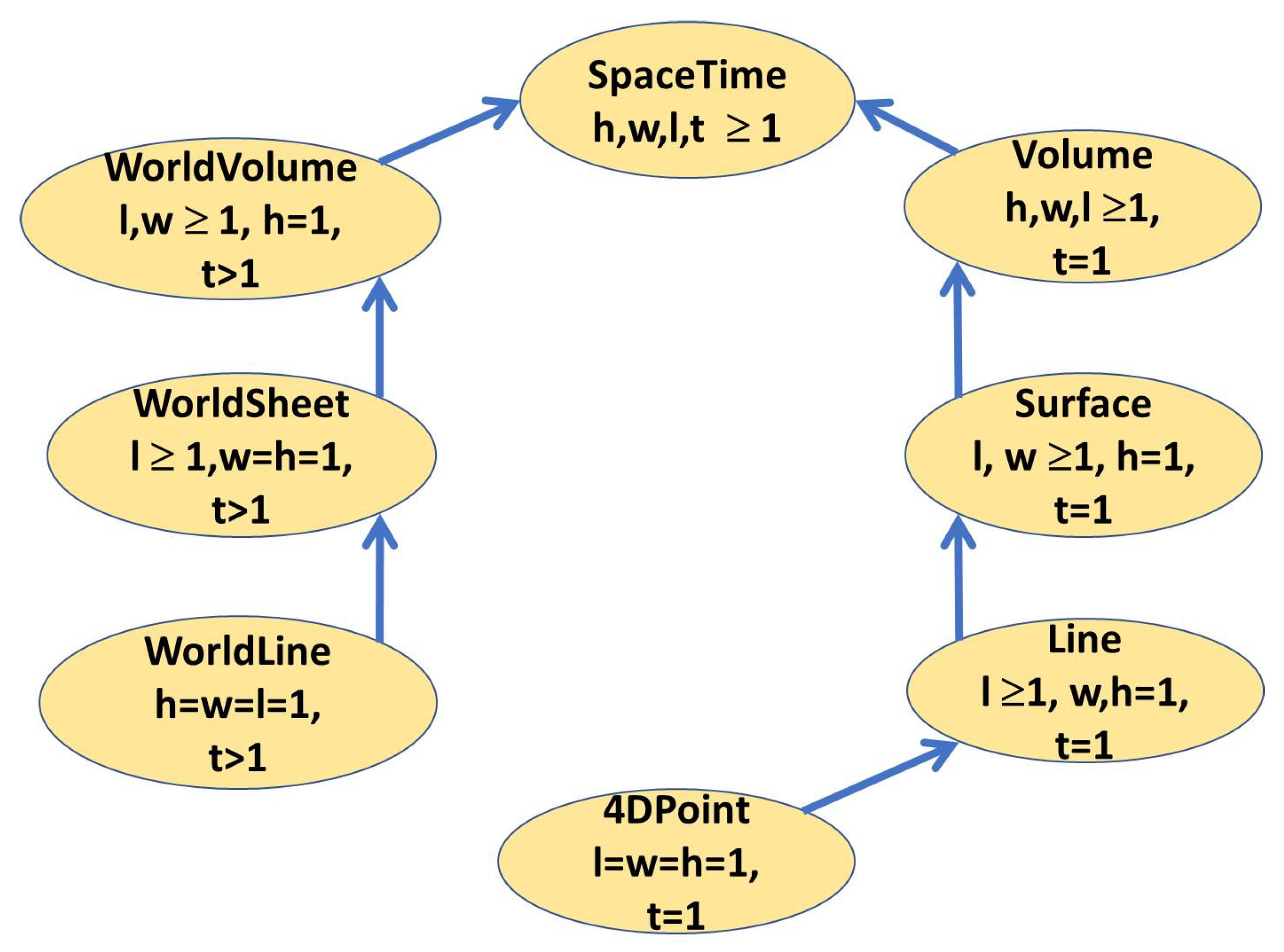
4] that “points”, as well as the other primitive notions in Euclidean geometry, such as “lines” and “planes”, do not have a separate existence in reality. As all of them are parts of a 4D-spacetime any of them—from a fundamental perspective—must have a 4D nature as well. Any (4D) SpaceTimeRegion isA 4DRegion, any 3DVolume isA 4DRegion being “thin” in the time dimension, any 2DPlane isA 4DRegion being “thin” in the time dimension and in one spatial dimension, and so forth (see Appendix A). Topology formalizes whether space–time regions (3D and/or 4D or even higher dimensional spaces) are connected items or not. If they are connected, some finite boundary region exists where they coexist and collocate.
Mereotopology finds application in the development of ontologies. Several foundational ontologies are based on mereotopology as one of the underlying concepts for the specification of relations between individuals and classes, with the most recent example being the Elementary Multiperspective Material Ontology EMMO [5]. Further standardized upper ontologies currently available for use include e.g., BFO [6], BORO method [7], Dublin Core [8], GFO [9], Cyc/OpenCyc/ResearchCyc [10], SUMO [11], UMBEL [12], UFO [13], DOLCE [14,15] and OMT/OPM [16,17].
The following section is adapted from [18] with slight modifications and amendments. In classical Euclidean geometry, the notion of “point” is taken as one of the basic primitive notions. In contrast, the Region-Based Theory of Space (RBTS), going back to Whitehead [3] and de Laguna [19], has as primitives the more realistic notion of a region as an abstraction of a finite-sized physical body, together with some basic relations and operations on regions, such as the isConnected or isPartOf relations. This is one of the reasons why the extension of mereology, complemented by these new relations, is commonly called mereotopology “MT”. There is no clear difference in the literature between RBTS and mereotopology, and by some authors RBTS is related, rather, to the so-called mereogeometry [20,21], while mereotopology is considered only as a kind of point-free topology, considering mainly topological properties of things. RBTS has applications in computer science because of its more simple way of representing qualitative spatial information. It initiated a special field in knowledge representation (KR) [22], called qualitative spatial representation and reasoning (QSRR) [23]. One of the most popular systems in QSRR is the Region Connection Calculus (RCC), introduced in [24]. The notion of Contact Algebra (CA) is one of the main tools in RBTS. This notion appears in the literature under different names and formulations as an extension of Boolean algebra with some mereotopological relations [25,26,27,28,29,30,31,32]. The simplest system, only called Contact Algebra (CA), was introduced in [31] as an extension of the Boolean algebra with a binary relation called “contact” and satisfying several simple axioms. Recent work addresses extensions of contact algebra [33].
Most of above approaches are based on monadic relations, such as Px (x isA Part), and dyadic relations, such as xCy (x isConnected y), and thus are limited to relations between two things. In the case of multiple things, higher-order relations may exist. An example might be a triadic relation, such as x isConnected y forSome z. A simple instance for such a relation would be, e.g., a motorway bridge connecting two cities on two sides of a river. If this bridge exists, the cities are connected for a car. Another example is catalysis, where the two chemical states, x and y, are connected (i.e., the reaction occurs) if a catalyst z is present. Otherwise, they are disconnected. These simple examples for triadic relations surely need a further formalization. According to Peirce’s Reduction Thesis, however, it can be stated, “(a) triads are necessary because genuinely triadic relations cannot be completely analyzed in terms of monadic and dyadic predicates, and (b) triads are sufficient because there are no genuinely tetradic or larger polyadic relations—all higher-arity n-adic relations can be analyzed in terms of triadic and lower-arity relations” (https://en.wikipedia.org/wiki/Semiotic_theory_of_Charles_Sanders_Peirce (accessed on 1 November 2021)). Proofs for Peirce’s Reduction Thesis are available, e.g., in [34,35].
The relation of an n-ary contact is described in a generalization of Contact Algebra called Sequent Algebra, which is considered as an extended mereotopology [36,37]. Sequent Algebra replaces the contact between two regions with a binary relation between finite sets of regions and a region satisfying some formal properties of the Tarski consequence relation. Another approach to multiple connected regions is, e.g., the mereology for connected structures [38].
Another important aspect, not yet covered by classical mereotopology, relates to the description of time-dependent relations and transitions. In normal language, this would refer to the specification of relations, such as “isConnected”, “wasConnected”, and hasBeenConnected”, or similar. The 4D-mereotopology [39] specifying, e.g., relations, such as “isHistoricalPartOf”, dynamic contact algebra DCA [40,41], and dynamic relational mereotopology [42], are current first approaches to tackle this challenge.
All of the above approaches to mereotopology are—to the best of the author’s knowledge—based on some Boolean algebra and additional relations. They thus only allow for qualitative descriptions, such as x isConnected y (or isNotConnected as the binary alternative). In contrast, the phase-field approach to mereotopology, depicted in the present article, allows the quantitative description of different “degrees of connectivity”, ranging, e.g., from 0% to 100%. The phase-field perspective thus provides a much higher expressivity and, in particular, allows for describing transitions—e.g., temporal changes—between classes that are disjoint in binary and Boolean relations. An example would be a transition from “isDisconnected” via different states of “isConnected” to “isProperPartOf” with a physics example for such a process being a cherry dropping into a region of whipped cream. Eventually, the formulation of relations, such as “wasConnected”, “hasBeenConnected” and many more, also becomes possible based on the same approach.
In the spirit of Whitehead’s Region-Based Theory of Space (RBTS), the regions in the phase-field model are defined by values of the phase-field. The phase-field is a scalar field that is defined over a continuous or discretized Euclidian space and thus has some relations with Discrete Mereotopology (DM) [43,44] and Mathematical Morphology MM [45]. An essay that also describes the discretized Euclidean space–time itself, based on mereology, is attempted in the Appendix B of the present article.
The major focus and innovative topics of the present article are (i) a step-by-step comparison of the logical (FOL) concepts of Boolean Algebra as used in mereology, region connect calculus and contact algebra with the algebraic and field theoretic concepts of the phase-field method, (ii) the identification of similarities and discrepancies between these two concepts for each of these steps, and (iii) the identification and preliminary discussion of the shortcomings of either method in a summarizing conclusion.

2. Scope and Outline

It is not the scope of the present article to review all the types of concepts mereotopology beyond what has shortly been summarized in the introduction. In addition, no comparison will be made with other important algebraic and numerical concepts addressing topology without explicitly drawing on fields, such as the cell method [46,47,48,49].
Mereotopology, mereogeometry and Region Connect Calculus all are based on logical expressions having only the logical values “true” or “false”. The phase-field concept—in contrast—allows for a quantitative and continuous description, particularly of the transitions between different regions. Following George Boolos: “to be is to be the value of a variable or some values of some variables” [50]; the value of the phase-field variable identifies anything as being a fraction of the universe or of a region under consideration. Any phase-field variable, accordingly, takes values from the closed interval [0, 1] of the real numbers, though in a strict sense “fractions” are all members of the set of rationale numbers.
The article starts from a short introduction into time-independent phase-field models, which represent objects/regions as scalar fields, namely, the so-called phase-fields. It will be demonstrated how boundaries can be represented as correlations of such scalar fields. Along with this basic introduction, analogies and correspondences to mereotopology will be indicated wherever possible and meaningful. A special section will discuss the extension of the description of dual-boundaries towards higher-order junctions, such as triple junctions and quadruple junctions, in which more than two things collocate and coexist.
A dedicated chapter—in a summarizing way—then compares expressions derived from the phase-field concept with their counterparts in region connect calculus and in classical mereotopology, respectively. It is, however, beyond the scope of the present article to discuss implications of the phase-field perspective for all types of more complex MT theories.
Current applications of the multiphase-field concept particularly address the evolution of complex structures in space and time. A dedicated section of the present article thus introduces the time perspective of the phase-field approach, leading to extended notions of isConnected, such as isTimeConnected (“coexistence”), isSpaceConnected (“collocation”), isPhysicallyConnected, and isCausallyConnected. Further notions become possible on the basis of the phase-field concept, such as wasPhysicallyConnected; isPathConnected, or isEnergeticallyConnected are shortly introduced and provide a promising outlook on possible future developments of mereotopology towards “mereophysics”.

3. Phase-Field Models

Not a single thing can be thought without a contrast to at least one other thing. Any thing thus has at least one “neighbor thing”. They form a boundary. They are connected. Multiple things form multiple dual boundaries, but also further lead to the formation of triple and quadruple boundary regions, where multiple things coexist and collocate. A method is successfully applied to describe objects; their shapes, and their boundaries are phase-field models that have been developed since the end of the last millennium.

3.1. Short History of Phase-Field Models

Phase-field models, in recent decades, have gained tremendous importance in the area of describing the evolution of complex structures, e.g., evolving during solidification of technical alloy systems [51,52] and their processing [53]. They belong to the class of theories of phase-transitions, which go back to van der Waals [54], Ginzburg-Landau [55], Cahn and Hillard [56], Allen and Cahn [57], and Kosterlitz-Thouless [58]. A phase-field concept was first proposed in a personal note [59] and later published by different authors [60,61]. The first numerical implementation of a phase-field model describing the evolution of complex-shaped 3D dendritic structures [62] attracted the attention of the materials science community. The concept was then further widened towards also treating multi-phase systems [63] and towards coupling with thermodynamic data [64]. Nowadays, a variety of simulation tools in the area of materials simulation draws on this concept, e.g., [65,66,67], and renders the evolution of complex structures and patterns—including the dynamics of boundaries and triple junctions—possible, Figure 1. Instructive reviews of phase-field modeling are available, e.g., in [68,69].

3.2. Basic Introduction to Phase-Field Models

The phase-field model, in the first place, is a way to mathematically describe things and their complex geometrical shape, as shown in Figure 2.
Similar to the Heaviside function Θ(x) [71], the phase-field function in one dimension Φ(x) is a function describing the presence or the absence of an object. However, in contrast to the Heaviside function, the phase-field function reveals a continuous transition over a finite —though very small—interface thickness η, Figure 3.
Nothing is a priori known about the exact “shape” of the phase-field function in the transition region. The reasoning towards a specification of this shape is based on statistical distributions of gradients in the interface and is described in [72,73]. In spite of not knowing this exact shape, a number of terms/expressions can already be qualitatively identified, as shown in Table 1, which allows the identification and description of the transition region (expressions (5), (6), (7:”overlap”), (8), (13), and (14) in Table 1), as shown in Figure 4.
An important characteristic of the phase-field description is that the terms (in expressions (4) and (12) in Table 1) corresponding to the “underlap” in mereology (expression (3)) sum up to a value of 1 everywhere and any time. Expressed in words, expression (4) reads:
The whole is the sum of its fractions—anywhere, at any time and in any subsystem.
Expressed as a formula, this reads:
1 = i = 0 N Φ Φ i ( x , t )     f o r   a l l   x   a n d   a l l   t     ( b a s i c   e q u a t i o n )
with NΦ being the number of things and Φ0 being the matrix/background thing [1].
In detail this equation—which has a very strong relation to the “mereological sum” defined in mereotopology (see Section 4)—means (i) that at least one thing is always present—i.e., has a non- zero value, (ii) that if a thing is the only—single—thing, it takes the value of exactly 1 (and all others take exactly the value 0), (iii) that if multiple things exist (i.e., have non-zero values), none of them reaches the value of 1, (iv) that if multiple things exist, their correlations also exist (expression 12) and (v) that if multiple things exist (i.e., have non-zero values) the sum of all their values equals to 1. Any transformation, any evolution, and any mereotopological description is subject to this “normalization” constraint.
To describe geometric structures, the phase-field function can be considered as being a function of space only. In this case, the function does not depend on time, and spatial structures are considered to be eternal and thus do not change. “Collocation”, then, is the key to describing boundaries and the relation isConnected becomes a synonym for isCollocated. “Collocation”, in the first place, requires the two things Φk and Φn to exist individually at the some—also existing—places xn and xl, which are tiny, but finite volumes inside the region of interest:
Φ i   e x i s t s   a t   x n   x n     Φ i ( x n )   0    
  Φ k   e x i s t s   a t   x l   x l   Φ k ( x l )   0
Φ i   i s C o l l o c a t e d   Φ k     x 0   s u c h   t h a t   Φ i ( x 0 ) 0   Φ k ( x 0 )   0
This expression describes the collocation of two things in a tiny volume x0. It is equivalent to a non-vanishing algebraic product describing the spatial correlation ΦiΦk in that tiny volume (see Table 1):
Φ i   i s C o l l o c a t e d   Φ k Φ i ( x 0 ) Φ k ( x 0 ) 0
The boundary between these two things thus can be defined as the set of all those volume elements xn, in which this correlation does not vanish. Summing up all these non-vanishing spatial correlations over all Nx tiny volumes xn constituting the overall volume of the system under consideration yields the fraction, which the dual boundary between Φi and Φk takes from that the total volume:
Φ i , k = 1 N x n = 1 N x Φ i ( x n ) Φ k ( x n )
The symbol has been introduced here to denote a boundary. This symbol is typically used in mathematics to denote the boundary Ω of a region Ω (see also the introduction of this notation in Table 1). The boundary between the two things, i and k—which is a volume—is related to the sum of all volume elements xn, where correlations between thing i and thing k are non-vanishing. Any of the things may also have further boundaries with other things. The total boundary of thing Φi then—in the lowest order of all its dual boundaries—is given by the sum of its dual boundaries with all ( ) other things:
Φ i , = 1 N x i = 0 i k N Φ j = 1 N x Φ i ( x j ) Φ k ( x j )
This is the same as:
Φ i , = k = 0 k i N Φ Φ i , k  
Φ i , k , as it is identical to 0, means that no interface at all exists between thing i and thing k: neither in the considered domain, nor in any of its sub-domains, nor in any of its elementary volume elements.

3.3. Multi-Phase-Field Models

Classical phase-field models—and most other theories of phase-transitions, as well as most mereotopological approaches—describe the boundary or connection between exactly two things (resp. the transition between exactly two states). In many areas of applications, however, situations occur, where three or more things coexist and collocate. An instructive practical example is the so-called peritectic reaction occurring during the solidification of a steel grade, as shown in Figure 5:
To account for such configurations, the multi-phase-field concept has been developed [63], which allows for the description of structures comprising multiple objects/things, such as different phases, as depicted in Figure 5, or for multiple grains of a single phase, as depicted in Figure 1. In this multi-phase-field model, the basic equation enters as a constraint into the Lagrange density, forming the basis for the derivation of the evolution equations for the different phase-fields.

3.4. Triple Junctions

Higher-order junction terms correspond to correlations of three (for triple junctions) or even more things (further, higher order junction terms). In multi-phase-field models triple junction terms are necessary to describe the equilibrium wetting angles, such as e.g., formed by a droplet on a solid substrate placed in the air, satisfying “Young’s Law” [74] and especially the kinetics of motion of such triple junctions. A detailed analysis of triple junctions and their role in phase-field models in microstructure evolution is given in [75].
As triple junctions are especially relevant for the description and discussion of “contacts” in the RCC and in mereotopology in Section 4, they are explicitly formulated here. For this purpose, the basic equation (expression (4) in Table 1) has to be formulated for at least three things and has to be—at least—cubed. Simple squaring of the basic equation even for three things will not generate triple junction terms.
1 = ( Φ i + Φ j + Φ k ) 3 = Φ i 3 + Φ i 2 Φ k + Φ i 2 Φ j + Φ i Φ k 2 + Φ i Φ j 2 + Φ i Φ j Φ k + Φ i Φ k Φ j            
( + + +   p e r m u t a t i o n s   o f   i , j , k )
The volume term (first term of the RHS) for the bulk fraction, where only the one object i exists, then reads:
Φ i = 1 N x n = 1 N x Φ i 3 ( x n )
The dual boundary fractions (second and fourth term for i and k, resp., third and fifth term for i and j) for the region i with the other region k in this ternary case then read:
Φ i , k = 1 N x n = 1 N x Φ i ( x n ) Φ k 2 ( x n ) + 1 N x n = 1 N x Φ i 2 ( x n ) Φ k ( x n )
This expression reduces to the binary case, if Φj = 0:
Φ i , k = n = 1 N x Φ i ( x n ) Φ k ( x n ) Φ k ( x n ) + n = 1 N x Φ i ( x n ) Φ i ( x n ) Φ k ( x n )
Φ i , k = n = 1 N x Φ i ( x n ) Φ k ( x n ) Φ k ( x n ) + Φ i ( x n ) Φ i ( x n ) Φ k ( x n )
Φ i , k = n = 1 N x Φ i ( x n ) Φ k ( x n ) [ Φ k ( x n ) + Φ i ( x n ) ]
With the sum in the square brackets being equal to 1 if Φj = 0:
Φ i , k = n = 1 N x Φ i ( x n ) Φ k ( x n )
The two ternary terms—the triple junction terms 6 and 7 on the RHS of the equation—contributing to the boundary of region i read:
Φ i , j , k = n = 1 N x Φ i ( x n ) Φ j ( x n ) Φ k ( x n )
and
Φ i , k , j = n = 1 N x Φ i ( x n ) Φ k ( x n ) Φ j ( x n )
These two terms—permuted in the last two indices—correspond to two different types of triple junctions, revealing a different helicity. The topic helicity is discussed in a separate section below. The total boundary of a thing i, then, is the sum of its dual boundaries plus the triple junction terms:
Φ i , = k = 0 k i 3 Φ i , k + j , k = 0 k i j 3 Φ i , j , k  
Based on these specifications of boundary and triple junction terms, mereotopological relations can be easily formulated and visualized based on some simple configurations, as will be shown in Section 4. It is important to note that all current mereotopological relations between two things will probably profit from the introduction/notion of a third thing, the “background” or “matrix” thing 0, to which they are connected as well, as shown in Figure 6.
The simple examples depicted in Figure 6 are introduced here to highlight the role of the “background” resp. “matrix” thing “0” and also the importance of triple and higher-order junctions for mereotopology in general. The class “no triple junction”, besides the case “isDisconnected”, also contains the case “isNonTangentialProperPart”; the class “one triple junction” applies to “isExternalContact” and also to “isTangentialProperPart”. Eventually, the presence of two triple junctions corresponds to the “isPartOf” relation.
Additional remark: The three configurations of things depicted in Figure 6 might also be considered as a temporal sequence of two individuals (“atoms”), as they are initially disconnected and then enter into a bound state. This scenario relates to Mulliken’s holistic interpretation of a bound state [76], where the two atomic orbitals must incorporate “the overlap in the space region that corresponds to the intersection of each atomic space” [77]. A mereology of quantum chemical systems has recently been discussed [78].
In the case of all three things being connected to each of the other things (see Figure 7, lower right, and Figure 8) there are three dual boundaries. Starting from the bottom and crossing these boundaries counter-clockwise, Figure 8 (left) displays the following sequence: red-blue, blue-green, and green-red, which we abbreviate for the ease of further reading as R-B, B-G, and G-R, or even simpler (also omitting the hyphens), as RB, BG, and GR. Thus, “RB” represents a transition from red to blue. This is definitely something to be distinguished from the transition “BR”—going from blue to red. Thus, RB is not the same as BR. The sequence of the symbols used to denote the boundary thus is important and has a meaning. It denotes the direction in which the boundary is crossed. Taking the convention of reading letters from left to right (as usual in most western languages) one will start from red to blue. In contrast, when taking the convention of reading signs from right to left (e.g., in the Arabian language), the red to green transition would be the first. Even more interesting, is to look at the sequence when going from one area to the next neighboring area. Again, starting on the bottom (the red region in Figure 8), the sequence reads R-B-G (and eventually back to red: -R). However, one could also start from blue and continue in so-called cyclic permutations:
R-B-G is the same as B-G-R is the same as G-R-B.
One will, however, never end (for this triple symbol AND when continuing going clockwise!) in a situation:
R-G-B is the same as G-B-R is the same as B-R-G.
The sequence of letters used to describe these two symbols—in two dimensions—thus either allows (i) the distinguishing of two different types of triple junctions or (ii) describes a sense of rotation (clockwise/counterclockwise), as shown in Figure 8, left and right.
Triple junctions are regions of collocation of three things. They are also regions where the three dual boundary planes (each of which is a volume that is thin in one direction) between the three different things collocate. As boundaries between any pair of two things in 3D are “planes”, the intersection of any pair of “planes” defines a “line” in three dimensions. Triple junctions thus are “lines” (having finite volumes), which in three dimensions either form closed loops—called vortices—or are connected to the boundary of the region of interest, respectively. Triple junctions are not “points”, as they seem to be in a 2D section, but lines. In 2D sections they always appear as “pairs”, as shown in Figure 9.
Figure 8. Two different triple junctions in 2 dimensions, in which three objects, red (R), green (G), and blue (B), coexist and collocate. They can be distinguished by the sequence in which the three things are arranged. They cannot be mapped onto each other by any rotation in 2D (see text), but only by mirroring. They may be—and in 3D physical systems probably are—connected in the third dimension (see text and Figure 10) meaning that they are parts of the same thing.
Appliedmath 02 00004 g008

3.5. Quadruple and Higher-Order Junctions

A maximum of four things can coexist at the same position “i.e., coexist and collocate”. In such a case they form quadruple “points”. Such quadruple points only exist in 3D space. Remember that all “points”, “lines” and “planes” are 3D objects (in a 3D world) resp. 4D objects in a 4D world (see Appendix A). There are:
  • Pairs of things forming dual boundaries (“planes”);
  • Three coexisting/collocated things forming three dual boundaries, coexisting/ collocated in a triple boundary (a “line”);
  • Four coexisting things have the following boundaries as parts, one quadruple “point”, four triple “line” junctions, and six dual boundary “planes”.
The fourth power of the basic equation for four things yields a total of 44 = 256 terms and can be sorted using the multinomial expansion (see e.g https://en.wikipedia.org/wiki/Multinomial_distribution (accessed on 1 November 2021)):
( Φ 1 + Φ 2 + Φ 3 + Φ 4 ) 4 = k 1 + k 2 + k 3 + k 4 = 4 4 ! k 1 ! k 2 ! k 3 ! k 4 ! Φ 1 k 1 Φ 2 k 2 Φ 2 k 3 Φ 4 k 4
The ki always sum up to four by definition of the sum. This is further detailed in Appendix C and eventually allows classifying into:
  • Four “unary” terms Φ i , —one of the ki equals four and the others are identical to 0;
  • A total of 84 “dual” boundary terms, where two of the ki are identical to 0 and the others complement four. For a dual boundary i,j this provides 14 terms: Φ i , j   ( seven   terms )   and   Φ j , i ( seven   terms ) . A total of six boundary pairs (i,j; i,k; i,l; k,l; j,k, and j,l) thus generates the total of 84 dual boundary terms.
  • A total of 144 “triple” boundary terms, where one of the ki is identical to 0 and the three others complement four. Each triple junction i,j,k generates 36 terms, which can be classified according to the helicity of the junction:
+ Φ i , j , k ( 18 terms ) + Φ i , j , k ( 18   terms ) = Φ i , j , k ( 36 t e r m s )
A total of four triple sets (i,j,k; i,j,l; i,k,l, and j,k,l) thus generates the total of 144 triple boundary terms.
A total of 24 “quadruple” boundary terms, where all ki are identical to one, leading to (sorted by the first index):
Φ i , j , k , l   ( 6   t e r m s ) ;   Φ j , i , k , l   ( 6 t e r m s ) ;   Φ k , i , j , l   ( 6 t e r m s ) ; Φ l , i , j , k   ( 6 t e r m s )
In summary, the following overall equation scheme results:
Φ i = Φ i + j i j Φ i , j + j , k i j k [ + Φ i , j , k + Φ i , j , k ] + j , k , l i j k l Φ i , j , k , l
Φ j = Φ j + i j j Φ j , i + i , k i j k [ + Φ j , i , k + Φ j , i , k ] + i , k , l i j k l Φ j , i , k , l
Φ k = Φ k + j j k Φ k , j + i , j i j k [ + Φ k , i , j + Φ k , j , i ] + i , j , l i j k l Φ i , j , k , l
Φ l = Φ l + j j l Φ l , j + j , k i j k [ + Φ i , j , k + Φ i , j , k ] + i , j , k i j k l Φ l , j , k , i
1 = i = 1 4 Φ i + i = 1 4 j j i Φ i , j + i = 1 4 j , k i j k [ + Φ i , j , k + Φ i , j , k ] + i , j , k , l i j k l Φ l , j , k , i
This eventually yields the total fractions of the four different objects (the LHS), as these are summed up from contributions of bulk, dual, triple, and quadruple boundaries. A visual impression of the different terms for bulks, dual boundaries, triple, and quadruple junctions is depicted in Figure 10.

3.6. Summary of Phase-Field Expressions

In view of the comparison with expressions from the region connect calculus, from contact algebra, and from mereology in the following sections, Table 2 provides a list of all the terms that are necessary for this purpose.
Looking at possible extensions to higher-order expressions, questions emerge, such as: Why not raise the basic equation to the sixth, to the eighth or to even higher powers? Is an even power mandatory? Why not go for more than four different objects? For a small number of objects (one, two, or three), an exponent equal to the number of objects seems sufficient. If only two objects exist, there will be no triple junction and an exponent of two can be considered as sufficient. As a first rule of thumb, the exponent should thus correspond to the number of objects. An exponent of four then seems sufficient—and necessary—to describe all types of geometric coexistence regions (the dual boundaries, “planes”; triple junctions, “lines”, and quadruple junctions, “points”) even if multiple objects are collocated. A power of six was used in [70] to refine the description of the dual interface in a solid–liquid two-state system by a refined discretization.

4. Comparison with Mereotopological Concepts

Based on the specifications of bulk areas, boundaries, triple junctions, and quadruple junctions depicted in the preceding section, especially in Table 2, mereotopological relations can easily be formulated and visualized based on some simple configurations, as outlined in the following.

4.1. Comparison with Region Connect Calculus

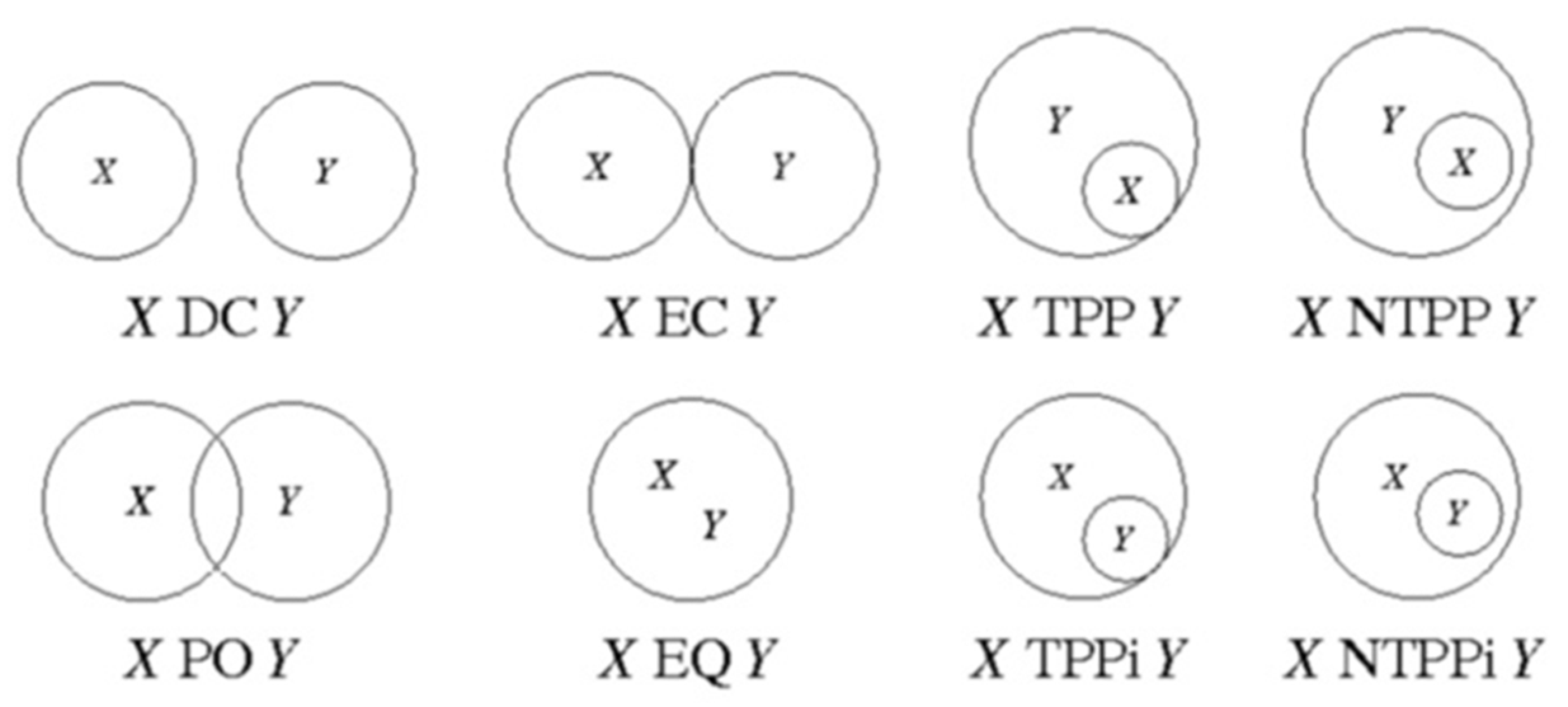
Some simple region connect calculus (RCC) situations, as shown in Figure 11, are individually discussed based on the description of boundary terms, as introduced in Section 3.
The discussion of these boundary terms will intentionally not follow the sequence as indicated in Figure 11. In contrast, it will start from the easily identifiable configurations (X DC Y, X NTTPi Y, X NTTP Y, and X PO Y), and then address the more complex situations involving only one Triple Junction (X EC Y, X TPP Y, and X TPPi Y). The most attention is eventually paid to X EQ Y.
Case: X DC Y: X and Y do not have any common boundary:
Φ x , y = 0
For X DC Y, parts X AND Y both have boundaries with the background thing 0 (not shown in the figure) only. Thus, their total boundary hasPart only of the boundary to the thing 0:
Φ x , = Φ x , 0 Φ y , = Φ y , 0
In addition, as there exists no dual boundary between X and Y, no triple junctions involving either of the two parts exist:
Φ x , y , 0 = 0                       Φ x , 0 , y = 0                       Φ y , 0 , x = 0                       Φ y , x , 0 = 0                            
Case: X NTPP Y: X has a boundary with Y only while Y has a boundary to thing 0 as well:
Φ x , = Φ x , y Φ y , = Φ y , x + Φ y , 0
Although there exists a boundary between both things, there is no region where both things are connected to the 0-thing as well. Thus, there are no triple junctions:
Φ x , y , 0 = 0                       Φ x , 0 , y = 0                       Φ y , 0 , x = 0                       Φ y , x , 0 = 0                            
Case: X NTPPi Y: Y has a boundary with X only while X has a boundary to thing 0 as well:
Φ x , = Φ x , y + Φ x , 0 Φ y , = Φ y , x
Though there exists a boundary between both parts, there is no region where both things are connected to the 0-thing as well. There are no triple junctions:
Φ x , y , 0 = 0                       Φ x , 0 , y = 0                       Φ y , 0 , x = 0                       Φ y , x , 0 = 0                            
All of the three cases above do not comprise any triple junction. The easiest case, including the triple junctions (X PO Y), will be discussed first, as this discussion is helpful in understanding the cases revealing only one single triple junction (i.e., the cases X EC Y, X TPP Y, and X TPPi Y).
Case: X PO Y: X and Y reveal a region of coexistence/collocation—the overlap region. A boundary between X and Y thus exists:
Φ x , y > 0
Further, both things X and Y in this case also have boundaries to thing 0:
Φ x , 0 > 0 Φ y , 0 > 0
X PO Y further comprises two regions (“points”), where all three things X AND Y AND the 0-thing collocate: there exist two triple junctions. Their total boundary thus hasPart of the boundaries to thing 0, to X (resp. to Y), and further, the two triple junctions, where X, Y, and 0 coexist/collocate. These two triple junctions, however, do NOT collocate—i.e., they exist in different volumes, xl and xm—and are distinguished by different helicities for the two different locations; see Section 3.4. A correlation of the two triple junctions does not exist in any volume element xn:
Φ y , = Φ y , 0 + Φ y , x + Φ y , x , 0 + Φ y , 0 , x
Φ x , = Φ x , 0 + Φ x , y + Φ x , y , 0 + Φ x , 0 , y
x l   : Φ x , y , 0 ( x l ) 0                         x m :   Φ x , 0 , y ( x m ) 0                         x n : Φ x , y , 0 ( x n ) Φ x , 0 , y ( x n ) = 0  
Case: X EC Y
In this case, there seemingly exists a single triple junction in a discretized single volume xn. This defines a “point” (a finite-sized smallest volume in two dimensions):
Φ y , 0 , x > 0
In the case of X PO Y, as discussed above, two triple junctions are coexistent—but not collocated. In the case of X DC Y, no triple junctions exist. X EC Y describes a transition between X DC Y and X PO Y, and thus benefits from being capable of describing both cases—each of them as a limit. Looking at the reverse process the two separated—i.e., not collocated—triple junctions in the X PO Y case then have to condense into a single state of coexistence AND collocate for the X EC Y case (and also for the TPP cases):
x n   :   Φ x , y , 0 ( x n ) 0                       Φ x , 0 , y ( x n ) 0                         x n : Φ x , y , 0 ( x n ) Φ x , 0 , y ( x n ) 0  
Case: X EQ Y
X and Y obviously have the same total boundary:
Φ x , = Φ y ,
Both have a boundary with 0 only:
Φ x , = Φ x , 0 Φ y , = Φ y , 0
Further, they both have identical phase fields:
  x n : Φ x ( x n ) = Φ y ( x n )
This expression directly implies that the two things are identical i.e., the “same thing” in a mereological sense. They have the same geometry, as defined by their individual phase fields. In terms of being fractions of a universe, both things are also identical. They can be treated as a single thing representing twice the fraction of one of the two things but losing their identity, then:
  x n : Φ z ( x n ) = Φ y ( x n ) + Φ x ( x n ) = 2 Φ x ( x n )
Further, there may be additional attributes beyond the mere geometric shape, which may still allow distinguishing them in spite of being geometrically identical.

4.2. Phase-Field Perspective of Contact Algebra

The topology axioms of contact algebra are (adapted from [18]):
(C1)
If aCb, then a > 0 and b > 0,
(C2)
If aCb and ac and bd, then cCd,
(C3)
If aC(b + c), then aCb or aCc,
(C4)
If aCb, then bCa,
(C5)
If ab ≠ 0, then aCb.
In the following, these axioms are related and compared to the phase-field formulations for time-independent situations. The phase-field formulations introduced in the preceding section are shortly recovered in the following for this purpose. A thing Φa is globally present in a region under consideration if it takes a non-zero value in this region:
Φ a > 0
A thing Φa is locally present in a region xj, which is a sub-region of the region under consideration, if it takes a non-zero value in that sub-region:
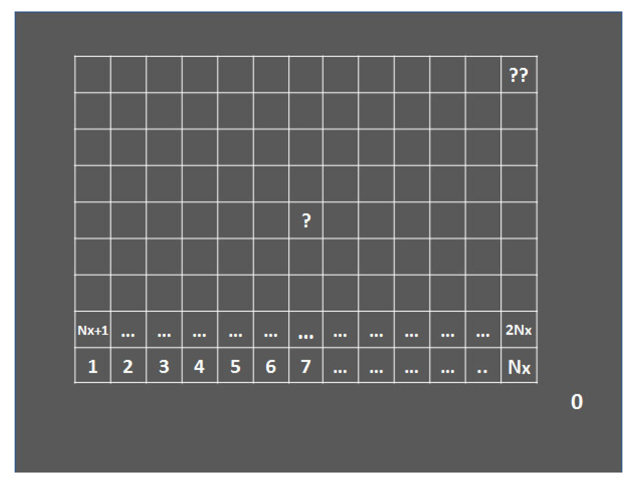
Φ a ( x j ) > 0
The global value Φa is the normalized sum of all local values in the Nx sub-regions:
Φ a = 1 N x j = 1 N x Φ a ( x j )  
Eventually the definition of “collocation” is:
Φ i   i s C o l l o c a t e d   Φ k     x 0   s u c h   t h a t   Φ i ( x 0 ) 0   Φ k ( x 0 )   0
This implies that there exists a boundary between the two things:
Φ i   i s C o l l o c a t e d   Φ k Φ i , k 0
Collocated” in this context (i.e., time independent) means “isSpatiallyConnected” or just isConnected, i.e., Φ i   C Φ k , in the nomenclature of contact algebra.
The Axiom (C1) of Contact Algebra—using the phase-field definition of isSpatiallyConnected—then translates into:
  Φ a   C Φ b   Φ a , b 0
Φ a , b 0     x n   s u c h   t h a t   Φ a ( x n ) 0   Φ b ( x n )   0
Φ a ( x n ) 0   j = 1 N x Φ a ( x j )   0   Φ a   0  
Φ b ( x n ) 0   j = 1 N x Φ b ( x j )   0   Φ b   0  
Φ a   C Φ b   Φ a   0       Φ b   0
Expressed in words, this reads: “If two things are locally connected, both things must at least globally exist”. Thus, Axiom (C1) is recovered by the phase-field perspective.
Axiom (C3) covers the case of one thing being connected to two other things, which both globally exist:
Φ a   0     Φ b   0     Φ c   0
Φ a   C   ( Φ b + Φ a )   x n   s u c h   t h a t   n = 1 N x Φ a ( x n )   [ j = 1 N x Φ b ( x n ) + k = 1 N x Φ c ( x n ) ] 0
n = 1 N x Φ a ( x n )   j = 1 N x Φ b ( x n ) + n = 1 N x Φ a ( x n ) k = 1 N x Φ c ( x n ) 0
n = 1 N x Φ a ( x n )   j = 1 N x Φ b ( x n ) 0             n = 1 N x Φ a ( x n ) k = 1 N x Φ a ( x n ) 0
    Φ a , b 0     Φ a , c 0     Φ a   C Φ b Φ a   C Φ c
Expressed in words, this reads: “If a thing is connected to two other things, it is connected to at least one of them”. Thus, Axiom (C3) is also recovered by the phase-field perspective. For multiple things this can be even further refined as: “Any thing is connected to at least one of the other things” or “Any thing is connected to its complement”.
Axiom (C4) relates to the symmetry of the connected relation:
Φ a   C Φ a     x n   s u c h   t h a t   Φ a ( x n ) 0   Φ b ( x n )   0
Φ a ( x n ) 0   Φ b ( x n )   0 Φ b ( x n ) 0   Φ a ( x n ) 0
Φ b ( x n ) 0   Φ a ( x n ) 0   Φ b   C Φ a
Expressed in words, this reads: “If thing “a” is connected to thing “b”, then thing “b” is also connected to thing “a””. Thus, Axiom (C4) is also recovered by the phase-field perspective for time-independent correlations.
The situation, however, may be—and probably is—different for time-dependence and other situations. A “path” connecting two things, “a” and “b”, may exist for some time, while the return path might not exist anymore, when attempting to go back from “b” to “a”. An example would be a bridge connecting “a” and “b”, which breaks down when crossing it for the first time. The concept of asymmetric connectivity has major implications for a number of areas in physics and chemistry, such as chemical reactions preferentially proceeding into one direction, entropy always increasing, or osmotic processes, to name a few. A simple example from everyday life is a one-way in traffic. To the best of the author’s knowledge a concept of asymmetric connectivity has not yet been discussed in any of the contemporary mereotopology endeavors. “Symmetric connectivity” can be retained by defining the two things, a and b, as isConnected, if at least one path direction does exist. This allows for a more general—even symmetric—formulation:
a, b are connecteda isPathConnected bb isPathConnected a
This expression, which is still symmetric, can be satisfied by following three configurations:
a isPathConnected bb ¬ isPathConnected a
a ¬ isPathConnected bb isPathConnected a
a isPathConnected bb isPathConnected a
The last expression indicates the existence of a reversible path, while both other expressions lead to irreversible situations, where there is a path from “a” to “b” (or vice versa), but no way back. Path connectivity is an important concept, introduced by Richard P. Feynman, and it finds applications in the principles of least action and/or Fermat’s principle. It is discussed in a little more detail in Section 5.5.
In a last but single step, Axiom (C5) is discussed, which essentially states that if two things globally exist, they are connected:
Φ a   0     Φ b   0     Φ a Φ b   0
Φ a Φ b = 1 N x 2 j = 1 N x Φ a ( x j ) k = 1 N x Φ a ( x k ) = 1 N x 2 ( k = 1 j = k N x Φ a ( x j ) Φ b ( x k ) + j , k = 1 j k N x Φ a ( x j ) Φ b ( x k ) ) 0
The second sum contains correlations between the volume elements xj and xk of the reference frame, when re-expressing the fields as products (i.e., Φ a ( x j ) Φ a x j ; see Appendix B.5). Neglecting such correlations (i.e., x j x k = 0 for all i,j), the second term on the RHS vanishes and only the first sum remains:
Φ a Φ b 0   k = 1 N x Φ a ( x k ) Φ b ( x k ) 0
k = 1 N x Φ a ( x k ) Φ b ( x k )   0     Φ a , b 0
Φ a , b 0     Φ a   C Φ b
As a side remark: In the spirit of the present article, such correlations will exist between volumes being in contact with each other, i.e., between neighboring positions. They are neglected here to show under which conditions the axioms of contact algebra can be recovered. These terms thus open options for a future refinement of the concept.
Expressed in words, this reads: “If two things globally exist, they are connected”. Thus, Axiom (C5) is also recovered by the phase-field perspective for the case of exactly two coexisting things. However, for three (and more things) existing globally, i.e., for:
Φ a   0     Φ b   0     Φ c   0
a number of options occurs which can be identified when using Axiom (C3):
Φ a   C ( Φ b + Φ c ) 0 Φ a Φ b + Φ a Φ c 0   Φ a Φ b 0   Φ a Φ c 0
Φ a   C Φ b Φ a   C Φ c
Thus—even if the two things, a and b, do exist globally (i.e., have non-zero values)—these two things, a and b, do not necessarily need to be connected if more than two things are globally present. In the case of a and b not being mutually connected, both have to be connected to—or separated by—a third thing, c. This directly implies the following global relations:
Φ a   0     Φ b   0       Φ c   0
Φ a , b   0       Φ a , c 0       Φ b , c 0
Expressed in words, this reads: “If three things globally exist, each of them is connected to at least one of the two other things”. Two things that are mutually connected directly imply that both exist globally (see Axiom C1):
Φ a C Φ b k = 1 N x Φ a ( x k ) Φ b ( x k ) 0 Φ a Φ b 0
Their individual global existence—in contrast, however—does NOT imply that they are connected if more than two things are considered. In the case of the three things, a, b, and c, two of them, e.g., a and b, may be mutually connected or may be disconnected (i.e., then separated by the third thing c):
Φ a Φ b 0   Φ a , b   0       Φ a , b = 0
Φ a , b = 0 Φ a ¬ C Φ b
If one of these boundaries does NOT exist (i.e., equals to 0) both other boundaries must exist (i.e., take non-zero values):
Φ a , b = 0       Φ a , c 0         Φ b , c 0  
If a triple junction exists, all three dual boundaries do exist:
Φ a , b , c 0     Φ a , b 0       Φ a , c 0           Φ b , c 0  
Thus, Axiom (C5) of contact algebra is recovered for exactly two existing things. The phase-field perspective depicted above seems, however, to imply that this axiom might have to be re-considered for the case of more than two things.
Eventually, Axiom (C2) will be discussed. This seems to be the most complicated discussion, as it involves four different things. The Axiom (C2): “if aCb and ac and bd, then cCd” expressed in words reads: If a isConnected b and a isPartOf c and if b isPartof d then c isConnected b. The individual expressions formulated in phase-field boundary terms translate into:
a C b   Φ a , b 0
If a isPartOf c, there exists a boundary between a and c:
a c   Φ a , c 0
The total boundary of “a” then hasPart of the two dual boundaries, but inevitably then also comprises a triple junction, a, b, and c:
Φ a , = Φ a , b + Φ a , c + Φ a , b , c
Then, further, b isPartOf d implies the existence of a boundary between b and d:
b d   Φ b , d 0
The total boundary of “b” then hasPart of the two dual boundaries, but inevitably also has a triple junction of a, b, and d:
Φ b , = Φ b , a + Φ b , d + Φ a , b , d
If aCb  t h e n     x n   s u c h   t h a t   Φ a , ( x n ) 0   Φ b , ( x n )   0
Φ a , b , d 0     Φ a , b , c 0 Φ a , b , c , d 0 Φ c , d 0   c C d
Accordingly, Axiom C2 can also be recovered by the phase-field perspective.
In summary, all five axioms of the axiomatic system of contact algebra can be expressed in terms of dual and higher order boundaries as described by the phase-field perspective.

4.3. Comparison with Mereology

While “connections” as used in region connect calculus and topology have been described as “boundaries” between things in the preceding chapter, the description of a “part” being at the heart of mereology is related to the phase field itself, in the phase-field perspective. The section starts with a short overview of mereology, as it is described in detail in [2].

4.3.1. Mereological Axioms and Definitions

Part: The monadic relation:
P x   x   i s A   P a r t
This defines “x” to be a part. This expression implies the existence of “x”, as in order to be a part, “x” must exist. It finds its phase-field counterpart in the expression.
a   i s A   P a r t Φ a   0
By intention, the phase-field notation here deviates from using “x” to denote a part as usual in mereology. In the context of the phase-field perspective, a, b, and c, etc., will be used instead. This is to avoid confusion with the xi being used to denote elementary spatial regions in the phase-field perspective. This implies that “a” (denoted as Φ a in the phase-field perspective) is a non-zero fraction of a system under consideration. The thing Φ a exists if it has a non-zero value and if the thing does not exist it takes the exact value of 0 [50]:
Φ a   e x i s t s   Φ a 0 Φ a   n o t E x i s t s   Φ a = 0
Parthood: Mereology further builds on a dyadic relation specifying parthood:
P x y   x   i s P a r t O f y
This parthood relation is considered as primitive following some basic axioms, such as (see, e.g., [2]):
P x x                               ( R e f l e x i v i t y ) P x y         P y x           x = y               ( A n t i s y m m e t r y ) P x y         P y z           P x z             ( T r a n s i t i v i t y )
Some commonly used definitions based on these axioms are
O x y         z ( P z x P z y )               ( O v e r l a p ) U x y         z ( P x z P y z )               ( U n d e r l a p ) PP x y     P x y     ¬   P y x                 ( P r o p e r P a r t h o o d )
Above axioms of ground mereology (M) are further complemented by a strong supplementation in extensional mereology (EM):
  ¬   P y x               z ( P z y ¬ O z x )   ( S t r o n g   S u p p l e m e n t a t i o n )
Then, extensional mereology is further complemented by the following closure extensional axioms, leading to closure extensional mereology (CEM):
U x y         z w ( O w z ( O w x   O w y ) )             ( S u m ) O x y         z w ( P w z ( P w x     P w x ) )             ( P r o d u c t ) z   x   P x z                 ( U p p e r   B o u n d )
Specifically, the individual z matching the upper-bound axiom fixes a universe u under consideration as a thing havingPart all parts:
u ! z   x   P x z                 ( U n i v e r s e )

4.3.2. An Essay towards a First-Order Logic Description of the Phase-Field Concept

The phase-field method to the best of knowledge of the author has not, by now, been formulated as an axiomatic system. The following section thus can be considered as a first essay towards formalizing the phase-field concept. It does not reveal the degree of maturity of the mereological axioms and is subject to future review. Before formulating the phase-field concept in FOL it is instructive to summarize the major concepts in their algebraic form.
In the phase-field concept all existing things are fractions and sum up to form the “whole” (i.e., the value 1). Non-existing things do not contribute to this sum, as their values are identical to 0.
Φ 0 + i = 1 N Φ Φ i = 1
The “complement thing”, Φ 0 , has been added to this sum to account for all the un-named or un-identified—but existing—fractions of the universe. The “complement thing” accordingly can be defined as:
Φ 0 1 i = 1 N Φ Φ i
The result is the basic equation already being introduced in [1] with the summation starting from i = 0:
i = 0 N Φ Φ i = 1   ( b a s i c   e q u a t i o n )
Without rigorous proof—which is beyond the scope of the present article—a number of implications can be directly inferred:
  • Postulating the number of things to be finite (NΦ) directly implies the existence of the smallest fraction that has no parts (i.e., an “atom”) and of the largest fraction (an “upper bound”);
  • If a thing is the only thing (the “whole”), it takes the value of 1 and its complement is 0 meaning that the complement does not exist;
  • If a thing is not the only thing, the complement exists (i.e., it has a non-zero value);
  • The basic equation corresponds to the mereological sum of all existing things (including the complement);
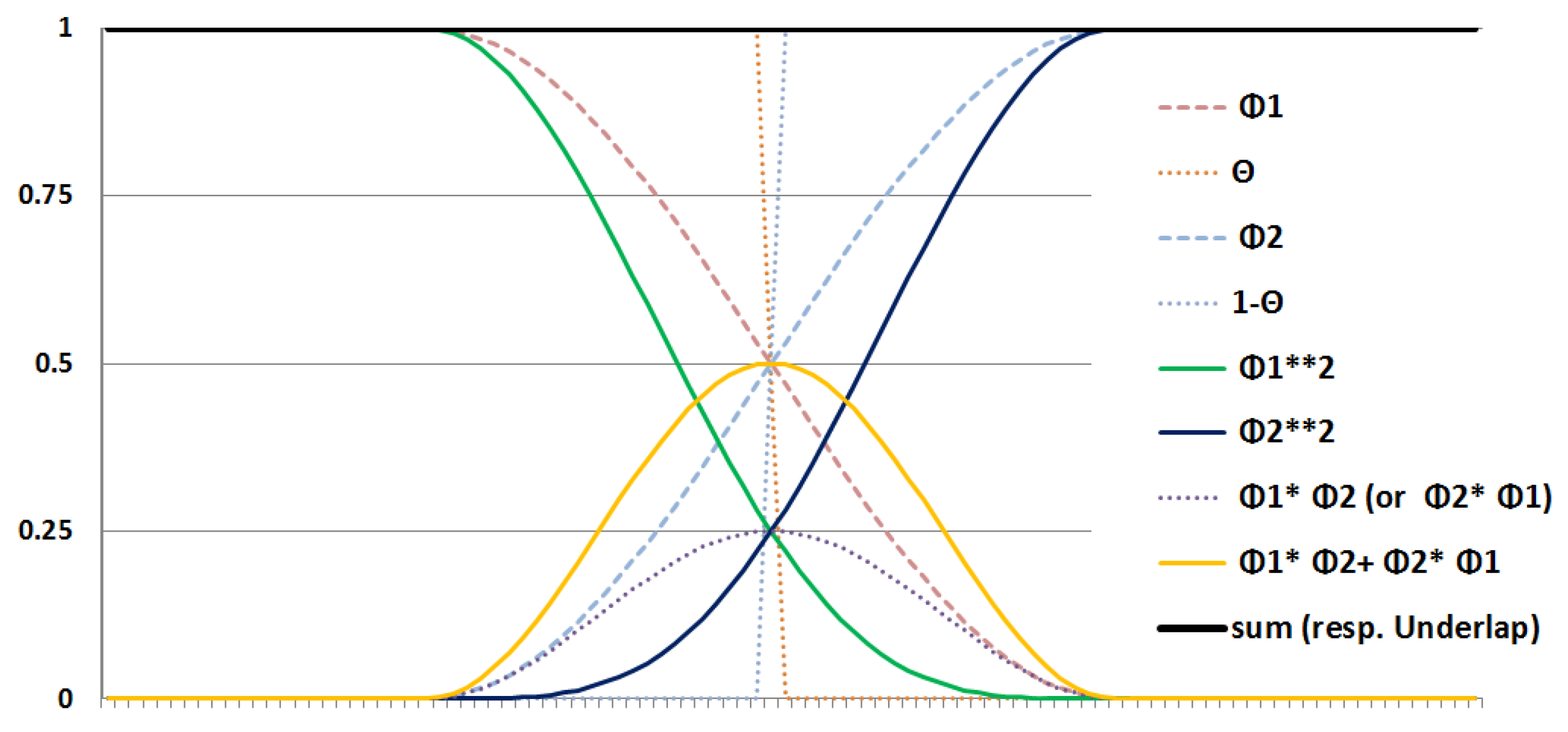
  • If both—a thing and its complement thing—exist, their—mereological—product (or their “boundary” or “correlation”) does exist and they are connected (see Section 4.2):
Φ i ¬ Φ i = Φ i ( 1 Φ i ) 0
Note that this correlation term between a thing and its complement is found in a number of areas. Examples are the logistic differential equation, where it corresponds to the derivative of the logistic function (https://en.wikipedia.org/wiki/Logistic_function (accessed on 1 November 2021)) and is named the logistic distribution:
f ( x ) = f ( x ) ( 1 f ( x ) )
The expression, interestingly, also corresponds to the lowest order Taylor approximation of entropy type terms [1]:
Φ i ( 1 Φ i )   ~   Φ i l n Φ i = S
In the following, a FOL description of the above concepts is attempted. For this purpose, the conventions of FOL are adapted and the Φ i are thus denoted as x, y, and z, etc., again in the following.
In the phase-field perspective all things—whether existing or non-existing (e.g., not yet or no longer existing)—are fractions (of a whole):
x     x [ 0 , 1 ]   ( f r a c t i o n s )  
The closed interval [0, 1] here is the interval of rationale numbers [ 0 , 1 ] , because any fraction by definition is a rationale number. In contrast to selecting the same interval of the real numbers [ 0 , 1 ] this implies that things are countable, as the set of rationale numbers is countable. In a refined axiomatization even a finite cardinality of the collection of N things could be postulated. If a thing exists it takes a non-zero value, if it does not exist it takes the value of 0:
x         x 0       ( e x i s t e n c e ) ¬ x         x = 0       ( n o n e x i s t e n c e ) x         x     ( 0 , 1 ]       x x = 1   ( 0 < x < 1 )
This provides a link between “Boolean Logics” and more general types of logic, such as Heyting logic (https://en.wikipedia.org/wiki/Intuitionistic_logic (accessed on 1 November 2021)) or Fuzzy logic (https://en.wikipedia.org/wiki/Fuzzy_logic (accessed on 1 November 2021)), allowing for multiple logic states beyond the binary Boolean alternative of ”true” and/or ”false”. The Boolean view is recovered if selecting the values from the interval of the natural numbers [ 0 , 1 ] , which only has the two elements 0 and 1 instead of [ 0 , 1 ] :
  t r u e   ( o r   B o o l e a n   I )   t r a n s l a t e s   i n t o   0   f a l s e   ( o r   B o o l e a n   0 )   t r a n s l a t e s   i n t o   = 0
For the rationale numbers we have for an existing thing:
x x = 1   ( 0 < x < 1 )
Expressed in words, this reads: if x exists (i.e., has a non zero value) it is either the whole (with a value of 1) or a part (with a value between 0 and 1). This allows for the specification of a whole and of a part in the following.
The whole corresponds to a unique, single object (universe) with no further objects existing, then:
  x   ( x = 1 )     ( W h o l e )
x = 1           y   ( ¬ y )     ( n o   f u r t h e r   t h i n g )  
The monadic part relation, as used, e.g., in mereology, is recovered by specifying “parts” as existing fractions (of a whole) with values smaller than one:
P x x < 1     x         (   P a r t   )
which is equivalent to x having a value in the open interval (0,1):
P x   x ( 0 , 1 )    
If x is a part or x does not exist, there exists at least one other fraction/thing:
P x   ¬ x           y     ( ( x + y < 1 ) ( x + y = 1 ) )         ( G e n e r a l   S u p p l e m e n t )
If x is a part, the “other” thing y is also a part:
P x       y   ( x + y 1 )       y   y < 1 )     P y
These two fractions either supplement each other to form a part, which still is not the whole:
x < 1       y     ( x + y < 1 ) ( S u p p l e m e n t )
x < 1           y     ( y < ¬ x )
or the two fractions x and y complement each other to form the whole:
¬ x   y   ( x + y = 1 ) ( C o m p l e m e n t )
  ¬ x   y   ( y = 1 x )
¬ x   ( 1 x )
The thing and its complement always complement each other to form the universe:
x ( x + ¬ x = 1 )     ( U n i v e r s a l   U n i o n )
which   compares   to
x ( x ¬ x = t r u e )     ( B o o l e a n )
The Universal Union allows inferring that the whole has no complement:
x = 1         ¬ x = 0     ¬ ¬ x     ( W h o l e   h a s   n o   c o m p l e m e n t )
In contrast to Boolean logic, a thing and its complement can coexist, i.e., they both can have non-zero values:
x : P x   ( x ¬ x 1 )   ( C o e x i s t e n c e )
This expression decomposes into two cases:
x   ¬ x 1 ( ( x   ¬ x = 0 ) ( x   ¬ x 0   ) )
Case (a) ( x   ¬ x = 0 )
For a binary interval of the natural numbers—i.e., the Boolean case—the only alternative for selecting “not being equal 1” is to be equal to 0. Case (a) thus reflects the Boolean view that a thing and its complement do not coexist:
x : x   ¬ x = 0   ( f a l s e )
The Boolean view thus is recovered in this special case. From the phase-field logic this expression reads:
( x   ¬ x = 0 ) ¬ ( x   ¬ x ) ¬ x ¬ ¬ x
x = 0   ¬ x = 0   x ¬ x = 0
Expressed in words, this reads that a thing and its complement do not coexist if either the thing or its complement do not exist individually.
Case (b) ( x   ¬ x 0 )
Case (b) is possible in a non-Boolean perspective only. In the phase-field formulation, one gets:
( x ¬ x 0 ) x ¬ x
x 0   ¬ x 0
x ¬ x 0
Note that ¬ x does NOT mean that x does not exist but ¬ x denotes the complement of x. In contrast: if x does not exist, its complement does exist and vice versa, via the General Supplement Axiom:
¬ x ¬ x
¬ ¬ x x
In the phase-field perspective, thus anything (!) which is a part overlaps (i.e., isConnectedTo) its complement part:
  O x ¬ x x   ( P x P ¬ x )   ( F u n d a m e n t a l   O v e r l a p )
This fundamental overlap is given by the algebraic product of the two non-zero fractions of the thing and its complement:
O x ¬ x x ¬ x  
O x ¬ x = x ( 1 x )  
The general overlap between two parts is defined as:
O x y   ( P x P y )   ( O v e r l a p ) O x y = x y
The overlap in the phase-field perspective corresponds to the situation of two things being connected, being collocated resp. two things having a boundary. Any part is connected to its complement in view of the fundamental overlap. If the complement of x has two parts, y and z, x is connected to at least one of them (see also the discussion of the Axiom C3 of contact algebra in Section 4.2):
O x ¬ x ( P ¬ x = P y P z )   P x ( P y P z )
P x ( P y P z ) ( P x P y ) ( P x P z )  
O x ¬ x = x y x z
A full FOL (First-Order Logic (https://en.wikipedia.org/wiki/First-order_logic (accessed on 1 November 2021))) or IPL (intuitionistic propositional logic (https://en.wikipedia.org/wiki/Intuitionistic_logic (accessed on 1 November 2021))) description of the phase-field concept is beyond the scope of the present article and will be the subject of a future, separate publication. It will include the definition of objects, such as triple and quadruple junctions, and interesting objects, such as the ratio of things.

4.3.3. Further Useful Definitions

The following section defines some further objects based on the closure extensional mereology (CEM) framework described in Section 4.3.1. The definition of these objects is helpful for a comparison with the phase-field perspective. The three objects being discussed for this purpose are the self-sum, the triple overlap, and the triple product.
Self-Sum: Formally interpreting the minimal underlap (i.e., the mereological sum) of a thing with itself leads to the following specification, which has not yet been used in mereology formulations to the best of the author’s knowledge:
U x x         z w ( O w z ( O w x   O w x ) )          
This expression reduces to:
U x x         z w ( O w z = O w x )             ( S e l f S u m )
This “self-sum” is observed to be identical with the fraction the part takes of the whole in the phase-field perspective.
Triple Overlap: A closer look at the “equivalence” in the expression for the mereological sum:
O w z ( O w x   O w y )
unveils three different options for Owz to be “true”:
      O w x = t r u e   O w y = f a l s e
O w x = f a l s e   O w y = t r u e
O w x = t r u e   O w y = t r u e
The last expression suggests—and allows for—a definition of a triple junction in the form of a triadic relation, which is not part of any mereology formulation by now. It is introduced here for the first time:
T x y z         w ( O w z O w x   O w y )             ( T r i p l e   O v e r l a p )
Expressed in words, this definition reads: “There exists a region w which overlaps with three regions x,y,z”. This region is denoted as a “triple overlap”.
Triple Product: Further, a maximum triple overlap—a “triple product”—comprising all regions w with triple overlaps of the same three things can be defined:
T x y z         t w ( O w z O w x   O w y )             ( T r i p l e   P r o d u c t )
The definitions of triple product and triple overlap are amended to classical mereology here, as they find their counterparts in the phase-field perspective (see table in Section 3.4).

4.3.4. Graphical Visualization of Mereological Expressions

Before eventually discussing mereology from the phase-field perspective, a graphical visualization of the different definitions in mereology is very instructive. Numerous graphical representations of the classical definitions and relations are available, e.g., Figure 12.
Some further graphics are added in the following allowing the discussion of some of the terms in more detail or trying to illustrate some of the terms graphically.
Underlap: The mereological underlap, Uxy, denotes a thing z, which has the two things, x and y, as parts. The two extremes are the whole (i.e., the universe individual) representing the maximum object comprising both things and the mereological sum representing the minimum object comprising both things, as shown in Figure 13.
However, there is no “unique underlap”. A variety of different objects fulfill the condition to be an underlap of two things. Between the two extremes depicted in Figure 13, a variety of different underlap objects can accordingly be defined, as shown in Figure 14.

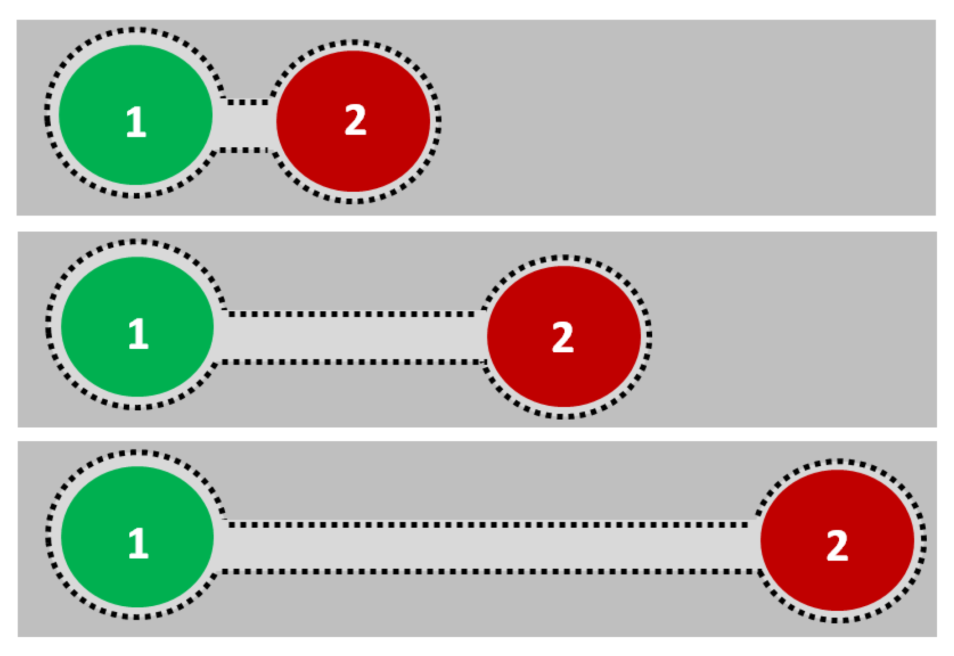
Self-Connected Underlaps of Disconnected Parts

If the underlap is postulated to be self-connected for both connected and also for disconnected things, a minimum of such a self-connected underlap can be used as a measure for distance, as shown in Figure 15. Further separating the two things will increase this minimal volume, while approaching them will decrease it. A distance, d, which also is a fraction of the universe, can thus be defined as the difference of the minimum self-connected underlap “MSCU” region and the “Mereological Sum”(MS, which is not self-connected for disconnected things). The value of d will become 0 in the case of external contact between the two things.
The volume of the minimum self-connected underlap (MSCU) will correspond to the sum of the underlaps of the individual parts (i.e., their mereological sum) plus a volume corresponding to the minimal string/path connecting the two parts (the path volume; see also Section 5.6) minus the total volume of their overlap (i.e., their mereological product). This concept is not addressed in current mereology, but can most probably be related to a concept of “potential energy”. Further discussion of this idea is beyond the scope of the current article and will be the subject of future work.

4.3.5. The Phase-Field Perspective of Mereological Expressions

An intuitive approach to a translation of mereological expressions to their phase-field counterparts starts from the mereological definition of the overlap:
O x y         z ( P z x P z y )               ( O v e r l a p )
The overlap in the phase-field perspective corresponds to the coexistence of the object Φ (denoted as x in the mereology expression) and an object of the reference frame xn (denoted y in the mereology expression). In the case of coexistence, both things are non-zero fractions of a universe, i.e., both have values in the open interval (0,1) of the rationale numbers. Their algebraic product (their correlation, “z” in the mereology expression, i.e., the overlap) thus exists:
Φ x n   0              
This allows defining the phase-field (or even any scalar field) as being the overlap of an object Φ and an object xn as being part of a reference frame. Without loss of generality, xn can exemplarily be imagined as a simple, individual voxel in a cubic grid.
Φ ( x n )   Φ x n                                 ( p h a s e f i e l d )
O w x     t r a n s l a t e s   i n t o     Φ x n   w h i c h     i s   t h e   l o c a l   p h a s e f i e l d   v a l u e   i n   x n :     Φ ( x n )
The mereological self-sum, which was introduced as the special case of the mereological sum in Section 4.3.3, can then be used to identify the total fraction of the object in the entire reference frame, being composed of “all xn
U x x         z w ( O w z = O w x )             ( s e l f s u m )
Identifying “all xn” (phase-field perspective) with “all w” (mereology) and x (mereology) with the object Φ (phase-field), facilitates the translation between the phase-field perspective and mereological expressions. The object z in this case is the total fraction of the object Φ. Assuming further “all xn” and thus “all w” to be countable and finite allows specifying the total fraction Φ of the object, which sums all xn where Φ is present.
Φ = 1 N x n = 1 N x Φ ( x n )
U x x     t r a n s l a t e s   i n t o   Φ ,   w h i c h     i s   t h e   g l o b a l   f r a c t i o n   o f   t h e   o b j e c t   Φ
Having thus related the phase-field expressions Φ ( x n ) and Φ (see Equation (1) in the table in Section 3.6) to mereological expressions, in the next steps the two expressions Φ i , k   and   Φ i , k ( x n ) (see Equation (3) in table in Section 3.6) will be discussed. They can be identified to relate to the mereological product. The mereological product is the largest overlap of two-phase fields describing the two things a and b, i.e., the region formed by all xn where the two things coexist. Things have been named a and b here in order not to generate confusion with the x denoting an existing object of the reference frame in the phase field perspective. The smallest region of coexistence—the smallest overlap—is defined by coexistence of the two things, at least in a single xn:
O a b   x n ( Φ a ( x n ) Φ b ( x n ) 0 )
Expressed words: There exists a volume xn which hasPart finite fractions of both parts a and b (or which isPart of both a and b):
O a b   x n (   P x n a     P x n b )  
This is the exact mereological definition of overlap and is also the phase-field definition of an interface in an elementary volume of the reference frame:
Φ a , b ( x n ) 0
O a b     t r a n s l a t e s   i n t o     Φ a , b ( x n )   w h i c h     i s   t h e   l o c a l   f r a c t i o n   o f   t h e     b o u n d a r y   b e t w e e n   a   a n d   b  
The maximum overlap—i.e., the mereological product—is the object comprising all xn, which contribute to the total boundary between the two things, a and b:
Φ a , b = 1 N x n = 1 N x Φ a , b ( x n )
T h e   m e r e o l o g i c a l   p r o d u c t   O a b     t r a n s l a t e s   i n t o     Φ a , b   w h i c h     i s   t h e   t o t a l   f r a c t i o n   t h e     b o u n d a r y   b e t w e e n   a   a n d   b   t a k e s   i n   t h e   u n i v e r s e   u n d e r   c o n s i d e r a t i o n  
Recovering the definition of the phase-field as the correlation (overlap) between the thing and a volume element xn of a reference frame (see Appendix B):
Φ a ( x n ) Φ a x n                   r e s p .                         Φ b ( x n ) Φ b x n
This allows the rewriting of O a b Φ a x n Φ b x n 0 , which can eventually be interpreted as a triadic relation: T a b x Φ a x n Φ b 0 . Expressed in words, this triadic relation reads: T a b x : a and b collocate in x. It can likewise be formulated for coexistence as T a b t : a and b coexist during t. Eventually, a quartic relation, Qabxt, for a physical contact, which corresponds to coexistence (during t) and collocation (in x) can be formulated: Q a b x t : a and b coexist in x during t.
The mereological sum—i.e., a possible, minimum thing, c, having the part two things, a and b—from a phase-field perspective—can directly be identified as the sum of the two individual phase-fields describing the two things, a and b, coexisting in an xn. The thing c—the sum—described by its own phase-field, then only has a and b as parts and no further thing:
Φ c ( x n ) = Φ a ( x n ) + Φ b ( x n )
U a b   ( U n d e r l a p )     i s   t h e   s a m e   a s     Φ a ( x n ) + Φ a ( x n )         ( s u m   o f   l o c a l     f r a c t i o n s )
Φ c = 1 N x n = 1 N x ( Φ a ( x n ) + Φ b ( x n ) ) = Φ a + Φ b
U a b   ( M e r e o l o g i c a l   s u m )     i s   t h e   s a m e   a s     Φ a + Φ b         ( s u m   o f   g l o b a l     f r a c t i o n s )

4.3.6. Graphical Comparison of Mereological and Phase-Field Descriptions

Boundary “areas” in mereotopology MT and in the region connect calculus RCC correspond to overlaps. External contact (EC) and tangential proper parts (TPP) both relate to triple junctions. There is no equivalent to quadruple junctions provided in either of these two concepts. The phase-field approach allows the description of mereotopological relations between things on the basis of the boundaries and the higher-order junctions they form, as shown in Figure 16 and Figure 17. Examples for three or more things forming a whole are depicted in Figure 18.
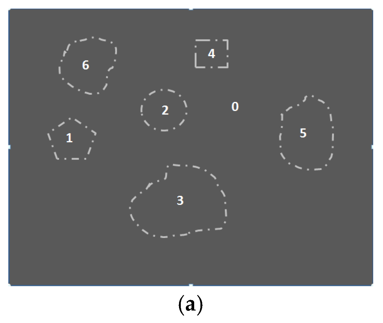
Based on boundaries, the topological relations between the things being depicted in Figure 16 can easily described. For example, thing 10 has an interface with the matrix 0 only: Φ 10 , = Φ 10 , 0 . Thing 1 is proper part of thing 2 and thus has an interface with 2 only: Φ 1 , = Φ 1 , 2 . Thing 2 (in the absence of thing 1) is a direct part of the universe (thing 0) and thus has an interface with 0 only: Φ 2 , = Φ 2 , 0 . In the presence of thing 1, however, thing 2 has an above external boundary with thing 0 but also a further internal boundary with thing 1: Φ 2 , = Φ 2 , 0 +   Φ 2 , 1 . Thing 4 is tangential part of thing 3 and thus has an interface with 3 only but also a single triple-junction: Φ 4 , = Φ 4 , 3 + Φ 4 , 3 , 0   Φ 4 , 0 , 3 . Things 5 and 6 represent a “bound state” and their boundaries are Φ 5 ,   =   Φ 5 , 0 + Φ 5 , 6 + Φ 5 , 6 , 0 + Φ 5 , 0 , 6 and Φ 6 ,   =   Φ 6 , 0 + Φ 6 , 5 + Φ 6 , 5 , 0 + Φ 6 , 0 , 5 .

5. Extended Notions of the isConnected Relation

Physics (from Ancient Greek: φυσική ) is the natural science that studies matter, its motion, and behavior through space and time. A concept of mereology/mereotopology addressing space AND time—i.e., a 4D mereotopology—similar to the MereoGeometry of 3D static structures—might thus be named MereoPhysics [1].
The phase field Φ in its typical applications is not only a function of space but a function of both space and time:
Φ k   e x i s t s   a t   x j   d u r i n g   t i   t i , x j     Φ k ( x j , t i )   0
This allows for a phase-field-based definition of “isConnected”(in 4D): Φ1 isConnected (in4D) to Φ2 if their correlation function is non-zero:
Φ 1 ( x 1 , t 1 )   i s C o n n e c t e d   Φ 2 ( x 2 , t 2 ) Φ 1 ( x 1 , t 1 ) P 2 ( x 2 , t 2 ) 0
This recovers the classical connectivity relation (C1) If aCb, then a > 0 and b > 0:
Φ 1 ( x 1 , t 1 ) Φ 2 ( x 2 , t 2 ) 0   Φ 1 ( x 1 , t 1 ) 0   Φ 2 ( x 2 , t 2 ) 0
Expressed in words, this relation reads: Any two things which (i) have existed, (ii) will exist or (iii) currently are existing in the 3D universe are (4D) connected. They may, however, exist at different times, i.e., they do “notCoexist” and thus are temporally disconnected. They also may coexist but may “notCollocate”, i.e., they may be spatially disconnected.

5.1. isTimeConnected: “Coexistence”

“Coexistence”, in the first place, requires two things to exist individually during some time intervals—ti,tl:
Φ k   e x i s t s   d u r i n g   t i   t i k ( t i )   0 Φ n   e x i s t s   d u r i n g   t l   t l n ( t l ) 0
Coexistence can then be defined as both things existing during the same time interval, t0:
Φ n   c o e x i s t s   Φ k     t 0   s u c h   t h a t   Φ k ( t 0 ) 0   n ( t 0 )   0
This is equivalent to a non-vanishing algebraic product describing the time-correlation ΦkΦn during that time interval, t0:
Φ n   c o e x i s t s   Φ k k ( t 0 ) n ( t 0 ) 0
Their temporal distance dt vanishes in this case because ti = tl (=t0):
d t   t i t l = 0

5.2. isSpaceConnected: “Collocation”

The aspect of “collocation” has already been addressed in Section 3 and Section 4, where mereotopology and the time-independent phase-field perspective were discussed in detail. In the case of time-dependent phenomena, 3D spatial connectivity is not static any more but becomes subject to change. The “isCollocated” relation thus needs to be complemented by a “wasCollocated” relation and in a similar way “coexists” needs a complement, such as “coexisted”. In addition, the relation “isPhysicallyConnected” introduced in the following section needs a complement relation, such as “wasPhysicallyConnected”. An instructive situation for such relations is depicted in Figure 19. Such relations can easily be formally defined based on the scheme depicted in Section 5.3. Although it would be possible to formally define relations for “willBeConnected” or similar relations directing to the future, this does not seem meaningful.

5.3. isPhysicallyConnected

Two things are physically connected if they share a common region of space x0 during a finite time interval t0 in which both are coexisting. They are coexisting and collocated in this case:
Φ n   i s P h y s i c a l l y C o n n e c t e d   Φ k   n   i s C o l l o c a t e d   Φ k           Φ n   c o e x i s t s   Φ k
Their phase-field description is a function of both variables, x and t, in this case.
Φ n   i s P h y s i c a l l y C o n n e c t e d   Φ k   x 0 , t 0   s u c h   t h a t   Φ k ( x 0 , t 0 ) 0   Φ n ( x 0 , t 0   ) 0
In a simple next step, even a relation “wasPhysicallyConnected“ can be defined for things which have formerly coexisted AND were collocated during a time interval tpast. They shared some former region x0 (remember x0 to be a finite region) during some past time interval tpast (tpast is also finite). “Now” (i.e., during a time interval, tnow) they arePhysicallyDisConnected:
Φ n   i s P h y s i c a l l y D i s C o n n e c t e d   Φ k   x 0 , t n o w   s u c h   t h a t   Φ k ( x 0 , t n o w ) 0   n ( x 0 , t n o w ) 0

5.4. isCausallyConnected

If two things are both spatially AND temporally disconnected—i.e., both their spatial AND their temporal distance do not vanish—they still may be connected by a relation isCausallyConnected. The situation is summarized in Figure 20:
If Equations (1) and (2) in Figure 20 are identical (i.e., c1 = c2 = c), they read:
c d t d x = 0
Equations (3) and (4) in Figure 20 are also identical if c3 = c4 = c, and then read:
  c d t + d x = 0
At least one of these equations is always satisfied, as the original four equations cover all possible combinations. The following expression, accordingly, is always “true”:
c d t d x = 0           c d t + d x = 0
These conditions together correspond to the solution of a quadratic equation and, accordingly, can be re-formulated and combined into a single equation:
( c d t d x ) ( c d t + d x ) = 0
This equation specifies the invariant space–time distance, ds2, known from special relativity theory to be equal to 0, as a criterion for things being causally (i.e., light-like) connected:
c 2 d t 2 d x 2 = 0 = d s 2

5.5. isEnergeticallyConnected

As an observation, there is a striking formal similarity between the invariant space–time interval and the energy–momentum balance of massless particles:
c 2 d t 2 d x 2 = 0 E 2 p 2 c 2 = 0    
Multiplying the first equation with a factor F2—which a priori shall only represent a conversion factor between spatial coordinates (first equation) and energetic perspective (second equation)—yields:
F 2 c 2 d t 2 F 2 d x 2 = 0  
Recovering the following expressions—actually the definitions—for energy E and momentum p—one immediately gets the second equation:
d E = F d x     a n d     d p = F d t                         d p 2 c 2 d E 2 = 0  
Much more interesting, however, is the definition of a relation, isEnergeticallyConnected, which means “equilibrium”. Any distance from the equilibrium then corresponds to a thermodynamic driving force, e.g., for phase transitions. Such a mereotopological view on thermodynamic equilibrium has quite recently been discussed [83].

5.6. isPathConnected

Regions where the thing Φi and an elementary region of the reference frame xj collocate can be described by a non-vanishing correlation (see Section 4 and Appendix B):
Φ i x j 0
Such a non-vanishing correlation holds for both of the following cases (see also Figure A5 in Appendix B):
x j   i s P r o p e r P a r t i                   O R             Φ i   i s P r o p e r P a r t   x j
If Φ isProperPart of xj the correlation denotes the position of this thing Φ, as the correlations of Φ with all other volume elements xk are identical to 0 in this case. This leads to:
k = 1 N x Φ i x k = Φ i x j x j Φ
This position may change over time. The time-dependent position is given by the coexistence of a time interval tj, the thing Φ, and the volume element xk:
Φ i x j t k 0
The position of a thing during the time interval tk (read “at time tk”) then can be written as:
x j Φ   ( t k ) x j Φ t k
Characteristic points of any path are its initial and final positions (the “start-point” and the “end-point”) denoting the two boundaries of a four-dimensional object being small in two spatial dimensions (a “line”—see Appendix A)—the “path”:
I n i t i t i o n P o s i t i o n :                     x i n i t i a l Φ x 0 Φ ( t 0 ) F i n a l P o s i t i o n :                     x f i n a l Φ x N Φ ( t N )  
An extended path then is a sequence of such positions bound by the initial and final positions, which all exist during a sequence of different time intervals, tk. The full path thus exists if any individual position has a non-zero value. For the extended path, this means that the product of all these positions is non-zero for a sequence of time intervals:
  A   p a t h   f r o m   x i n i t i a l Φ   t o   x f i n a l Φ     e x i s t s     k = 0 N x k Φ ( t k )   0
The total “path” of a tiny point-like (i.e., smaller than the volume element xk) thing between two positions x i n i t i a l Φ and x f i n a l Φ taken by the thing at two different times, 0 and N, then can be summed up, yielding the total volume P of the path “line”:
P Φ ( x 0 , x N ) = k = 0 N x k Φ ( t k )
Any position x k Φ is a fraction of the whole and thus has a value smaller than 1. The probability of a path to exist (which is given by the above product) thus decreases with the increasing number, N, of path elements forming the product. This fact leads to a higher probability for shorter paths with the minimum path length being the most probable path. This is most likely related to the principle of least action and Fermat’s principle. The sum and the product expressions find continuum counterparts in the Feynman path integrals, (https://en.wikipedia.org/wiki/Path_integral_formulation (accessed on 1 November 2021)) with a rigorous formal comparison being subject to future work. The interesting fact here seems that these expressions are derived based on mere logic considerations.

6. Summary, Conclusions and Outlook

The present article has related and compared the concepts of mereotopology, region connect calculus and contact algebra to a field-theoretic description of objects, their shapes, and their boundaries by the phase-field concept. The concepts underlying mereotopology, on the one hand, seemed to be similar to the principles underlying the phase-field concept, on the other hand, a number of differences/complementarities became obvious.
In the first place, some limitations of Boolean algebra were identified. Boolean algebra does not allow for the coexistence of a thing and its complement. Such a coexistence, however, is essential not only in the phase-field perspective, where coexistence and collocation are actually measures for the physical boundary between things. Mereotopology is based on Boolean algebra and thus considers the different types of connectivity as logically—and thus qualitatively—disjoint. Transitions, e.g., from “x isDisconnected y” to “x isProperPartof y”—with a cherry dropping into whipped cream being an example—thus cannot or can only hardly be addressed. Transitions, however, are ubiquitous processes and thus need a formal description. Such a description may widen the field of applications of contemporary mereology, mereotopology and mereogeometry, towards new grounds of mereophysics.
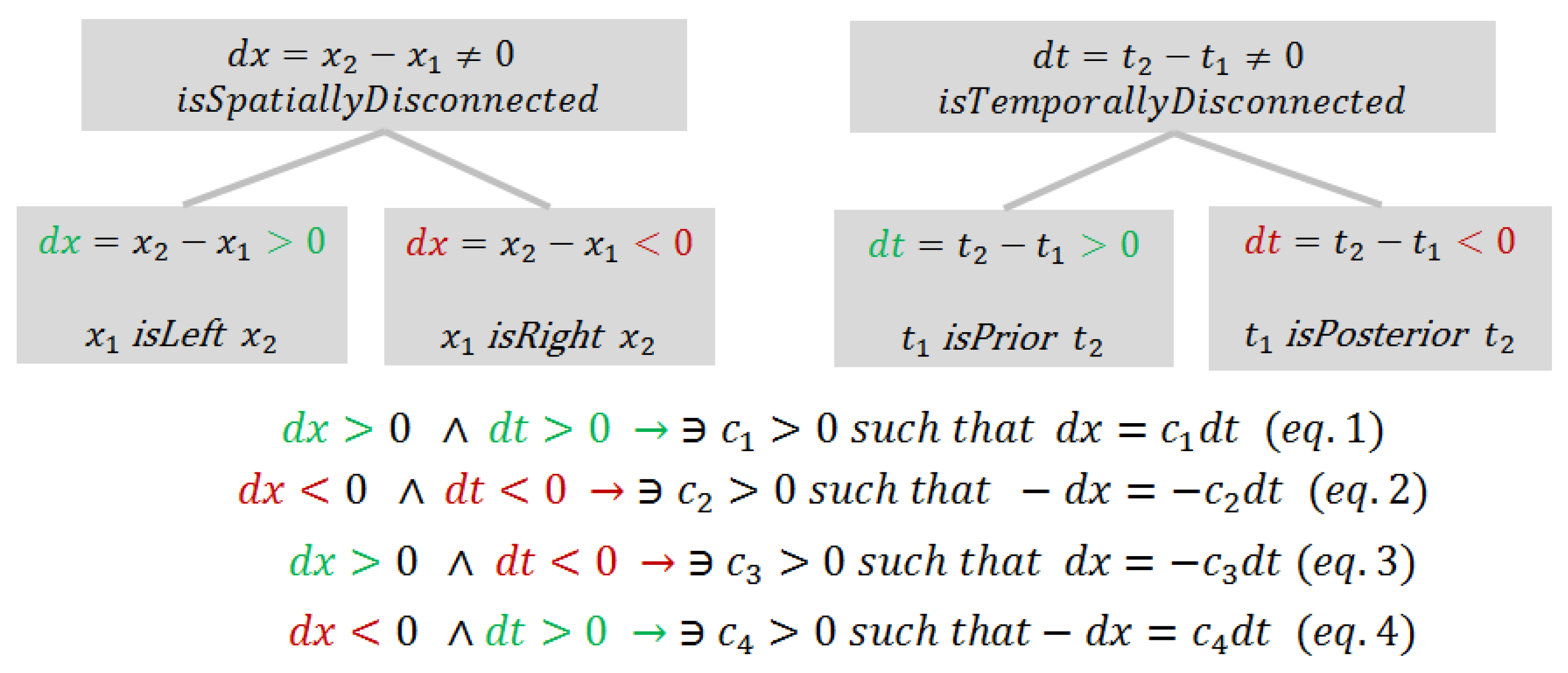
A “dynamic” view on contacts and boundaries and the notion of time were thus introduced. This is first reflected in time-dependent relations allowing one to semantically describe “historicalParthood” via “isConnected” or “wasConnected” relations. Separating the description of 4D connectivity into “isSpatiallyConnected” and “isTemporallyConnected” allowed for the definition of “isPhysciallyConnected” and eventually also of “isCausallyConnected”. As a consequence, the formulation of the relativistic space–time interval could be derived from mere logical inference.
Eventually the symmetry of the connectivity relation was discussed, where an “isPathConnected” and an “isEnergeticallyConnected” relation provide the grounds for describing reversible and/or irreversible paths.
In a generalized notion, the “isConnected” relation, according to the present article might be interpreted as some generalized “distance” between two things to be equal to 0. This generalized distance may be a spatial distance, a temporal distance, an energetic distance or any other type of general distance. All these distances are expressed as the difference between two values. Thus the status of “isConnected” is reached if two values are equal, i.e., if two values satisfy the equation of type A − B = 0. A possible notion of “distance” was introduced, which could be described in mereological terms as minimal self-connected underlap minus the mereological sum of two disconnected things.
Concepts of higher-order junctions were discussed. These relate to the connectivity of more than two things. The benefits of describing triple junctions with triadic relations and the importance of triadic relations in general were highlighted as well as the notion of helicity and aspects of 3D connectivity of triple junctions being seemingly disconnected in 2D. A potential need to reconsider/reformulate one of the axioms in contact algebra was identified when discussing the connectivity of multiple objects.

Funding

The work presented in this article is a spin-off from discussions during the formulation of the Elementary Multiperspective Material Ontology EMMO and from discussions on applications of EMMO for Metamodels and Digital Shadows within the WorkStream AII of the Cluster of Excellence “Internet of Production” funded by the Deutsche Forschungsgemeinschaft DFG under the grant [EXC 2023, Project-ID: 39062112].

Institutional Review Board Statement

Not applicable.

Informed Consent Statement

Not applicable.

Data Availability Statement

Not applicable.

Acknowledgments

The author thanks Emanuele Ghedini, Jesper Friis, Gerhard Goldbeck, Adham Hashibon, and Sebastiano Moruzzi for their patience and for all the interesting and constructive discussions on philosophy and on various areas of physics during the intense work on EMMO.

Conflicts of Interest

The author declares no conflict of interest. The funders had no role in the design of the study; in the collection, analyses, or interpretation of data; in the writing of the manuscript, or in the decision to publish the results.

Appendix A. 4D Geometry

This appendix proposes a solution to the dilemma of describing points, lines, surfaces, and volumes known from classical geometry—all with different dimensions there—all as 4D physicals. Based on a recent essay to derive physics laws from mereology [1] and the mereological principle that any part of a 4D item again has to be a 4D item, the basic approach to a solution is shortly outlined in the following in a very simplified way.
Any volume in 3D V3D is the product of a length L, a width W, and a height H and can be written as a scalar triple product:
H e z ( L e x × W e y ) = V 3 D
Further assuming the length L (and width W and height H) being—integer—multiples of an elementary length scale lp, allows the rewriting of:
h e z ( l e x × w e y ) l p 3 = V 3 D   w i t h   i n t e g e r s     h , l , w 1
The volumes being thin in one of the three spatial dimensions—i.e., surfaces—then, are defined as 3D volumes, where exactly one of the integers takes the value of 1. Lines correspond to 3D volumes, where exactly two of these integers take the value of 1 and the points are elementary volumes, in which all three integers take the value of 1.
The time T, as fourth dimension, becomes a further factor in the product defining the volume in 4D (V4D). cT is an integer multiple of a length scale lp = cτp:
V 4 D = V 3 D c T = V 3 D t c τ p w i t h   i n t e g e r   t 1
All of the objects in the following scheme, as shown in Figure A1, are accordingly, 4D space–time items:
Figure A1. Concept to integrate different 4D objects (”points”, “lines”, and “surfaces”) as subclasses of a 4D physical space–time. The classes are differentiated by the values of the variables l, w, h, and t (see text). Arrows are to be read as “isPartOf” relations.
Appliedmath 02 00004 g0a1

Appendix B. From Mereology to a Scalar Field

Appendix B.1. Reference Frame

To obtain information about the local existence or non-existence of things, their mutual positions, and their topological arrangement in a region of spacetime, it is beneficial to discretize this region into smaller sub-regions specifying a “reference frame” or a “coordinate system”.

Appendix B.2. Discretization of Spacetime

Multiplying the basic equation (which is based on the top axiom of mereology [1]) with a pseudoscalar entity, such as, e.g., a volume V, is the first step towards discretizing space:
i = 0 N Φ Φ i V = i = 0 N Φ V i = V
V represents the total volume of the universe under consideration. Note that this volume and all the sub-regions V i are pseudoscalars (Figure A2a). In a next step, tiny—elementary—cubes, all with the same size—may be considered as abstracted regions. These do not need to be interconnected but might be embedded in an unstructured matrix (Figure A2b and Figure A3c).
Figure A2. (a) The shape size of the abstract sub-regions a priori is arbitrary. They do not need to be interconnected, regular shaped, or have the same size. Actually, the abstract sub-regions could also be the volumes covered by the different things themselves. (b) As these sub-regions are abstract regions they may be considered as tiny—elementary—cubes, all with the same size. Still, they do not need to be interconnected but might only be embedded in an unstructured matrix 0 (dark). They may reveal different orientations.
Appliedmath 02 00004 g0a2aAppliedmath 02 00004 g0a2b

Appendix B.3. “Self-Assembly” of Spacetime

In a further step, the cubes can be arranged—or may by some process self-assemble—into a regular lattice. This process might be interpreted as a condensation of a structured volume from an unstructured gas phase containing individual volumes. In an intermediate step, molecule type arrangements of volume elements may form, as shown in Figure A3a:
Figure A3. (a) “Molecules” of crystallized space–time forming the initial nucleus for a space–time lattice. (b) Arranged—or by some process self-assembled—cubes in a regular lattice. Their names (indices) are a priori random, and cube #2 does not necessarily have to be a neighbor of cube #1. Note, the volume outside the structured grid is filled by an “unstructured matrix” volume 0, to recover the entire original region of space (dark). (c) In contrast to (b) the cubes—though arranged in a regular lattice—in this situation, are separated by a “foam” of the matrix thing 0. Such a configuration appears quite frequent in nature, e.g., atoms in a crystal being separated by vacuum/fields. In this case, all xi are connected to the matrix thing only and do not have any direct correlations.
Appliedmath 02 00004 g0a3
The number N of things in Figure A3 is the total number of cubes, which for a—cube/brick type—reference frame is N x N y N z , see Figure A4. Actually, the region under consideration here is composed of a structured grid and an unstructured matrix, V0.
All cube volumes, Vi, for i  > 0 are identical with respect to their value and only differ with respect to their position in the lattice being denoted by their name/index j. V0 fills all possible empty space between the cubes and also the remaining parts of the volume of the universe not filled by the cubes.
V 0   + j = 1 N x N y N z V j = V  
If nothing exists in volume 0, everything exists in the structured volume. The total volume can then be re-sized to the structured part, V, only:
j = 1 N x N y N z V j = V    
A speculative side remark: Comparing this “self-assembly” process with a crystallization process, further suggests the possible release of some latent heat, which might be the initial energy present during the big bang (which would be a big nucleation and crystallization process and not an explosion in this picture).

Appendix B.4. Neighborhood Relations

The names/indices of the individual volume elements in the preceding section were selected arbitrarily. A simple renaming does not affect the volume elements, except by changing their name. By convention, naming the indices of the cubes allows for the introduction of neighborhoods, e.g., cube #5 is the left neighbor of cube #6 and right neighbor of cube #4 in a linear, one-dimensional chain of cubes. This naming scheme can easily also be extended to 3D, as shown in Figure A4.
Figure A4. A linear naming scheme can also be extended to 2D and 3D. In this 2D example, Nx is 13 and Ny is 9. The index of cell “?” is 4 × 13 + 7 = 59 and cell “??” has the value Nx × Ny = 9 × 13 = 117. Cube #5 would obtain cube #18 (Nx + 5) as an additional neighbor (“top”-neighbor) in this 2D example.
Appliedmath 02 00004 g0a4
This naming step is the most important, as it introduces and defines “left” and “right” (in one dimension) and also front/rear and top/bottom in three dimensions. Such neighborhood relations are essential and open up the possibility to describe the relative positions of things.

Appendix B.5. Positions and Scalar Fields

For a 3D situation, the number of the cubes is NxNyNz. The index has been switched to j here to distinguish it from the index, i being is used to count the things Φi. The volume of the structured space–time, V’, is only considered in the following.
j = 1 N x N y N z V j V = 1
This equation can be directly multiplied with the basic equation for the –scalar– things Φ i yielding:
j = 1 N x N y N z V j V   i = 0 N Φ Φ i = 1
j = 1 N x N y N z i = 0 N Φ V j Φ i = V
For a single thing in the vacuum/matrix ( N Φ =1), that is represented on this “grid”, this equation reads:
j = 1 N x N y N z i = 0 1 V j Φ i = V
j = 1 N x N y N z ( V j Φ 1 + V j Φ 0 ) = V
The term
V j Φ 1 Φ 1 ( V j )  
is the correlation between the elementary cube volume, Vj, and the thing 1. This product only exists where both Vj and Φ1 coexist, i.e., where both have non-zero values.
The value of the index j corresponds to a well-defined position, rj, of the centroid of the cube j, as defined by the numbering/naming scheme that is detailed above. The equation, accordingly, defines a discretized field describing the presence of thing 1 at various, discrete positions, rj:
V j Φ 1 Φ 1 ( V j ) = Φ 1 ( r j )  
If the volume of the Φ1 is smaller than the volume element Vj, this correlation will only exist inside this particular volume, Vj, and the term then defines the position of the thing, Φi:
V j Φ 1 = V j ( Φ 1 ) = r j ( Φ 1 )           f o r           Φ 1 < V j  
These two cases are illustrated in Figure A5:
Figure A5. Left: If Φ (red) isProperPart of a specific volume element xj (depicted by the black boundary) this particular volume element defines the position of Φ up to some remaining uncertainty. Right: All volume elements xj, being parts of Φ, denote regions where Φ is present. If they are ProperParts of Φ, there is no other thing present in this particular volume element.
Appliedmath 02 00004 g0a5
If the thing Φ1 is bigger than an individual Vj, the total volume of the thing i then reads:
j = 0 N x N y N z V j Φ 1 = V 1  
Remark: This equation in a continuum formulation corresponds to:
0 V Φ 1 ( r ) d x d y d z = V 1  
In a next step, the time intervals can be introduced by multiplying the basic equation with a scalar (not a pseudoscalar), called time T:
k = 0 N t Φ k T = T k = 0 N t t k = T  
Similar to the selection of identical volumes, identically sized time intervals can also be selected, making the index k a measure for the position of the respective time interval on the arrow of time. A volume Vj exists during a time interval tk, which means:
V j t k > 1  
This is a 4D space–time volume element. Thing i exists during a time interval tk, which means:
Φ i t k > 1  
“Coexisting” eventually means that the correlation is also a correlation with the time interval, making the product not vanish during that time interval:
V j Φ 1 t k > 1  
Eventually, a scalar field description for a—discretized—scalar field describing the elementary regions covered can be formulated:
V j Φ 1 t k = Φ 1 ( V j , t k )    
where, in a continuous formulation (with Vj and tk → 0), it can be identified with a scalar field—the phase-field:
Φ 1 ( r j ,   t k ) Φ 1 ( r ,   t )  

Appendix C. States and Interface States

Quadruple junctions—i.e., the collocation of four things—correspond to “points” (which are still finite-sized volumes). Looking at the fourth-order exponents of the basic equation raised to the fourth power thus can be expected to yield further insights:
1 = ( Φ i + Φ J + Φ K + Φ L ) 4
This yields a total of 44 = 256 terms, which can be sorted using the multinomial expansion (https://en.wikipedia.org/wiki/Multinomial_theorem (accessed on 1 November 2021)):
( Φ 1 + Φ 2 + Φ 3   + Φ 4 ) 4 = k 1 + k 2 + k 3 + k 4 = 4   4 ! k 1 ! k 2 ! k 3 ! k 4 ! Φ 1 k 1 Φ 2 k 2 Φ 3 k 3 Φ 4 k 4
The ki always sum up to four by definition. This allows classifying into:
  • Four “unary” terms Φ i with one of the ki being equal to 4 and all others being identical to 0;
  • A total of 84 “dual” boundary terms, where two of the ki are identical to 0 and the others complement 4;
  • A total of 144 “triple” boundary terms, where one of the ki is identical to 0 and the three others complement 4;
  • 24 “quadruple” boundary terms, where all ki are identical to 1;
Unary states:
One ki = 4 and the others equal to 0, which yields a total of four states:
4 ! 4 ! 0 ! 0 ! 0 ! Φ 1 4   ,     4 ! 0 ! 4 ! 0 ! 0 ! Φ 2 4 ,     4 !   0 ! 0 ! 4 ! 0 ! Φ 3 4 ,     4 ! 0 ! 0 ! 0 ! 4 ! Φ 4 4
Dual boundaries:
Two ki = 0 e.g., k3 = 0 ∧ k4 = 0.
(i) Two other k are identical and complement to 4 e.g., k1 = k2 = 2
4 ! 2 ! 2 ! 0 ! 0 ! = 6 6   d u a l   b o u n d a r i e s = 36
(ii) Two other k are different and complement to 4 e.g., k1 = 1 ∧ k2 = 3 or k1 = 3 ∧ k2= 1
4 ! 1 ! 3 ! 0 ! 0 ! = 4 6   d u a l   b o u n d a r i e s = 24
4 ! 3 ! 1 ! 0 ! 0 ! = 4 6   d u a l   b o u n d a r i e s = 24
In total, the description of a dual boundary i,k thus comprises three types of linear independent states (   i . e . , Φ i 2 Φ k 2   ; Φ i 3 Φ k 1   a n d   Φ i 1 Φ k 3 ), which might be related to a “pseudo-vector” perpendicular to the boundary. A total of six dual boundaries exists: (k3 = 0 ∧ k4 = 0 ∨ k2 = 0 ∧ k4 = 0 ∨ k1 = 0 ∧ k4 = 0 ∨ k2 = 0 ∧ k3 = 0 ∨ k2 = 0 ∧ k1 = 0 ∨ k1 = 0 ∧ k3 = 0)
Ternary junctions:
One of the ki = 0 (e.g., k4), two ki = 1 and one ki = 2.
There is a total of four triple junctions (i.e., k1 = 0 ∨ k2 = 0 ∨ k3 = 0 ∨ k4 = 0):
4 ! 1 ! 1 ! 2 ! 0 ! = 12 4     t r i p l e   j u n c t i o n s = 48
4 ! 1 ! 2 ! 1 ! 0 ! = 12 4   t r i p l e   j u n c t t i o n s = 48
4 ! 2 ! 1 ! 1 ! 0 ! = 12 4   t r i p l e   j u n c t t i o n s = 48
In total, the description of a ternary junction i,j,k (a “triple boundary”) thus also comprises three linear independent states ( i . e . ,   Φ i 1   Φ j 1 Φ k 2 ; Φ i 1   Φ j 2 Φ k 1   a n d   Φ i 2   Φ j 1 Φ k 1 ) , which might be related to a “vector” parallel to the triple boundary line.
Quaternary Junction
All ki are equal: (k1 = k2 = k3 = k4 = 1):
4 ! 1 ! 1 ! 1 ! 1 ! = 24
Some simplifications of the above expressions are possible. The general unary term for object i is:
Φ i = k i = 4 k j = k k = k l = 0 4 ! k i ! k j ! k k ! k l ! Φ i k i Φ j k j Φ k k k Φ l k l
This simplifies to:
Φ i = Φ i 4
The dual boundary terms for a single boundary between i and j:
Φ i , j = k i + k j = 4 k k = k l = 0 4 ! k i ! k j ! k k ! k l ! Φ i k i Φ j k j Φ k k k Φ l k l
simplify to:
Φ i , j = k i + k j = 4 4 ! k i ! k j ! 0 ! 0 ! Φ i k i Φ j k j Φ k 0 Φ l 0
and further to:
Φ i , j = k i + k j = 4 4 ! k i ! k j ! Φ i k i Φ j k j
This term then simplifies and splits into:
Φ i , j = k i = k j = 2 4 ! 2 ! 2 ! Φ i 2 Φ j 2 = 6 Φ i 2 Φ j 2
plus:
k i = 3     k j = 1 4 ! 3 ! 1 ! Φ i 3 Φ j 1 = 4 Φ i 3 Φ j 1
and:
k i = 1     k j = 3 4 ! 1 ! 3 ! Φ i 3 Φ j 1 = 4 Φ i 1 Φ j 3
The triple junction terms for junctions involving i, j, and k (i.e. kl = 0):
Φ i , j , k = k i + k j + k k = 4 k l = 0 4 ! k i ! k j ! k k ! k l ! Φ i k i Φ j k j Φ k k k Φ l k l
simplify to:
Φ i , j , k = k i + k j + k k = 4 4 ! k i ! k j ! k k ! Φ i k i Φ j k j Φ k k k
and can be split into:
Φ i , j , k = k i = 2 k j = k k = 1 4 ! 2 ! 1 ! 1 ! Φ i 2 Φ j 1 Φ k 1 = 12 Φ i 2 Φ j 1 Φ k 1
plus:
k j = 2 k i = k k = 1 4 ! 1 ! 2 ! 1 ! Φ i 1 Φ j 2 Φ k 1 = 12 Φ i 1 Φ j 2 Φ k 1
and:
k k = 2 k i = k j = 1 4 ! 1 ! 1 ! 2 ! Φ i 1 Φ j 1 Φ k 2 = 12 Φ i 1 Φ j 1 Φ k 2
These triple junction terms eventually sum in total to:
Φ i , j , k = 12 Φ i 2 Φ j 1 Φ k 1 + 12 Φ i 1 Φ j 2 Φ k 1 + 12 Φ i 1 Φ j 1 Φ k 2
These can be split into cylic and anticyclic permutations:
Φ i , j , k = + Φ i , j , k + + Φ i , k , j = ( 6 Φ i 2 Φ j 1 Φ k 1 + 6 Φ i 1 Φ j 2 Φ k 1 + 6 Φ i 1 Φ j 1 Φ k 2 ) + ( 6 Φ i 2 Φ k 1 Φ j 1 + 6 Φ i 1 Φ k 2 Φ j 1 + 6 Φ i 1 Φ k 1 Φ j 2 )
The “6” ahead of each of the terms correspond to the number of cyclic permutations of the i, j, and k. This can be rewritten by introducing the two helicities (see Section 3.4) into:
+ Φ i , j , k + Φ i , j , k = Φ i , j , k
using the following definition:
Φ i , j , k = + Φ i , k , j

Appendix D. Construction of an Item from Mereotopological/Phase Field Information

The scope of this appendix is to provide the solution to the challenge posed in Section 4.3.6 and to discuss further options for a refined description of a geometrical state. The information provided for the solution of the challenge is listed again in the following table. The aim was to describe the well-known Tai-Chi symbol (a) based on connectivity. A description of connectivity is necessary but not sufficient to describe this symbol. Symbol (b) would have the same topological description. The phase-field concept brings further information about the relative sizes of the objects. The fraction object 1 takes of the universe shall be equal to the fraction object 2 takes and the same holds for objects 3 and 4) ( Φ 1 = Φ 2     Φ 3 = Φ 4 ). In addition, the relative fractions of interfaces may be used as criteria. Note that the equal sign indicates the fractions the object take of the universe to be identical, but not the objects themselves. This further constrains the possible choices of a geometrical configuration matching all conditions but still does not lead to the Tai-Chi Symbol (c). Further constraints can be placed on the ratio of the surface (with finite thickness) to the area (remember that in mereology both have the same dimension) leading to a description of disc-type objects (d). This brings the description of the Tai-Chi symbol closer to the desired object. Still, many things, such as “distances” or “orientations”, are missing. Figuring out possible descriptions for further constraints is subject to future efforts.
Appliedmath 02 00004 g0a6

References

  1. Schmitz, G.J. Quantitative mereology: An essay to align physics laws with a philosophical concept. Phys. Essays 2020, 33, 479. [Google Scholar] [CrossRef]
  2. Casati, R.; Varzi, A.C. Parts and Places; MIT Press: Cambridge, MA, USA, 1999; ISBN 9780262517072. [Google Scholar]
  3. Whitehead, A.N. Process and Reality; MacMillan: New York, NY, USA, 1929. [Google Scholar]
  4. Schulz, D.R. Platonism, Mereology and Whitehead’s Process Ontology; Monash University: Monash, Australia, 2015; Available online: https://bridges.monash.edu/articles/thesis/Platonism_mereology_and_Whitehead_s_process_ontology/4719385 (accessed on 1 November 2021).
  5. Ghedini, E.; Goldbeck, G.; Hashibon, A.; Schmitz, G.J.; Friis, J. EMMO: The Elementary Multiperspective Materials Ontology. 2021. Available online: https://github.com/emmo-repo/EMMO (accessed on 1 November 2021).
  6. Arp, R.; Smith, B.; Spear, A.D. Building Ontologies with Basic Formal Ontology; MIT Press: Cambridge, MA, USA, 2015; ISBN 9780262527811. [Google Scholar]
  7. BORO—the Business Objects Reference Ontology. Available online: https://en.wikipedia.org/wiki/BORO (accessed on 1 November 2021).
  8. Available online: https://en.wikipedia.org/wiki/Dublin_Core (accessed on 1 November 2021).
  9. Herre, H.; Heller, B.; Burek, P.; Hoehndorf, R.; Loebe, F.; Michalek, H. General Formal Ontology (GFO): A Foundational Ontology Integrating Objects and Processes. Part I: Basic Principles. Research Group Ontologies in Medicine (Onto-Med); University of Leipzig: Leipzig, Germany, 2008. [Google Scholar]
  10. Available online: https://en.wikipedia.org/wiki/Cyc (accessed on 1 November 2021).
  11. Available online: https://en.wikipedia.org/wiki/Suggested_Upper_Merged_Ontology (accessed on 1 November 2021).
  12. Available online: https://en.wikipedia.org/wiki/UMBEL (accessed on 1 November 2021).
  13. Nardi, J.C.; Falbo, R.D.A.; Almeida, J.P.A.; Guizzardi, G.; Pires, L.F.; van Sinderen, M.J.; Guarino, N. Towards a commitment-based reference ontology for services. In Proceedings of the Enterprise Distributed Object Computing Conference (EDOC), 2013 17th IEEE International, Vancouver, BC, Canada, 9–13 September 2013; pp. 175–184. [Google Scholar]
  14. Gangemi, A.; Guarino, N.; Masolo, C.; Oltramari, A.; Schneider, L. Sweetening Ontologies with DOLCE. In Knowledge Engineering and Knowledge Management: Ontologies and the Semantic Web; Gómez-Pérez, A., Benjamins, V.R., Eds.; Springer: Berlin/Heidelberg, Germany, 2002; pp. 166–181. [Google Scholar] [CrossRef]
  15. Borgo, S.; Masolo, C. Ontological Foundations of DOLCE. In Theory and Applications of Ontology: Computer Applications; Springer Science+Business Media B.V.: New York, NY, USA. [CrossRef]
  16. Available online: https://en.wikipedia.org/wiki/Object_Process_Methodology (accessed on 1 November 2021).
  17. Dori, D. Object-Process Methodology: A Holistic Systems Paradigm; Springer Science & Business Media: Berlin/Heidelberg, Germany; ISBN 9783642562099.
  18. Ivanova, T. Extended Contact Algebras and Internal Connectedness. Studia Log. 2019, 108, 239–254. [Google Scholar] [CrossRef]
  19. de Laguna, T. Point, line and surface as sets of solids. J. Philos. 1922, 19, 449–461. [Google Scholar] [CrossRef]
  20. Borgo, S.; Masolo, C. Full Mereogeometries. Rev. Symb. Log. 2010, 3, 521–567. [Google Scholar] [CrossRef] [Green Version]
  21. Borgo, S.; Ferrario, R.; Masolo, C.; Oltramari, A. Mereogeometry and Pictorial Morphology. Image Ausg. 2007, 536–550. [Google Scholar]
  22. Levesque, H.J. Readings in Knowledge Representation; Morgan Kaufmann: Burlington, MA, USA; ISBN 978-0-934613-01-9.
  23. Stell, J.G. Mereotopology and Computational Representations of the Body. Comput. Cult. 2017, 6, 1–21. [Google Scholar]
  24. Randell, D.A.; Cui, Z.; Cohn, A.G. A spatial logic based on regions and connection. In Proceedings of the 3rd International Conference Knowledge Representation and Reasoning, Los Altos, CA, USA, 25–29 October 1992; Nebel, B., Swartout, W., Rich, C., Eds.; Morgan Kaufmann: Burlington, MA, USA, 1992; p. 165. [Google Scholar]
  25. de Vries, H. Compact Spaces and Compactications. Ph.D. Thesis, University of Amsterdam, Amsterdam, The Netherlands, 1962. [Google Scholar]
  26. Stell, J.G. Boolean connection algebras: A new approach to the Region Connection Calculus. Artif. Intell. 2000, 122, 111–136. [Google Scholar] [CrossRef] [Green Version]
  27. Vakarelov, D.; Düntsch, I.; Bennett, B. A note on proximity spaces and connection based mereology. In Proceedings of the 2nd International Conference on Formal Ontology in Information Systems (FOIS’01), Ogunquit, ME, USA, 17–19 October 2001; Welty, C., Smith, B., Eds.; ACM: New York, NY, USA, 2001; pp. 139–150. [Google Scholar]
  28. Vakarelov, D.; Dimov, G.; Düntsch, I.; Bennett, B. A Proximity Approach to Some Region-Based Theories of Space. J. Appl. Non-Class. Logics 2002, 12, 527–559. [Google Scholar] [CrossRef]
  29. Bennett, B.; Düntsch, I. Axioms, Algebras and Topology. In Handbook of Spatial Logics; Aiello, M., Pratt, I., van Benthem, J., Eds.; Springer: Berlin/Heidelberg, Germany, 2007; pp. 99–160. [Google Scholar]
  30. Düntsch, I.; Winter, M. A representation theorem for Boolean contact algebras. Theor. Comput. Sci. 2005, 347, 498–512. [Google Scholar] [CrossRef] [Green Version]
  31. Dimov, G.; Vakarelov, D. Contact algebras and region based theory of space: A proximity approach I. Fundam. Inform. 2006, 74, 209–249. [Google Scholar]
  32. Düntsch, I.; Vakarelov, D. Region-based theory of discrete spaces: A proximity approach. Ann. Math. Artif. Intell. 2007, 49, 5–14. [Google Scholar] [CrossRef]
  33. Balbiani, P.; Ivanova, T. Relational Representation Theorems for Extended Contact Algebras. Stud. Logica 2020, 109, 701–723. [Google Scholar] [CrossRef]
  34. Burch, R. A Peircean Reduction Thesis: The Foundations of Topological Logic; Texas Tech University Press: Lubbock, TX, USA, 1991. [Google Scholar]
  35. Correia, J.H.; Pöschel, R. The Teridentity and Peircean Algebraic Logic. In Conceptual Structures: Inspiration and Application; ICCS 2006. Lecture Notes in Computer Science; Schärfe, H., Hitzler, P., Øhrstrøm, P., Eds.; Springer: Berlin/Heidelberg, Germany, 2006; Volume 4068. [Google Scholar] [CrossRef]
  36. Vakarelov, D. A mereotopology based on sequent algebras. J. Appl. Non-Class. Log. 2017, 27, 342–364. [Google Scholar] [CrossRef]
  37. Vakarelov, D. Extended Mereotopology Based on Sequent Algebras. Available online: https://www.dc.fi.udc.es/~cabalar/LRC16/slides/Vakarelov_LFworkshop-Vakarelov.pdf (accessed on 1 November 2021).
  38. Grüniger, M.; Chui, C.; Ru, Y.; Thai, J. A Mereology for Connected Structures. In Formal Ontology in Information Systems; Brodaric, B., Neuhaus, F., Eds.; IOS Press: Amsterdam, The Netherlands. [CrossRef]
  39. Stell, J.G.; West, M. A 4-Dimensionalist Mereotopology. Available online: https://www.researchgate.net/publication/249754393_A_4-Dimensionalist_Mereotopology (accessed on 1 November 2021).
  40. Vakarelov, D. Point-Free Theories of Space and Time. arXiv 2020, arXiv:2004.14755. [Google Scholar]
  41. Available online: https://www.researchgate.net/project/Mereotopology-static-and-dynamic (accessed on 1 November 2021).
  42. Nenchev, V. Dynamic relational mereotopology: Logics for stable and unstable relations. Log. Log. Philos. 2013, 22, 295–325. [Google Scholar] [CrossRef]
  43. Galton, A. The mereotopology of discrete space. In Spatial Information Theory: Cognitive and Computational Foundations of Geographic Science; Freska, C., Mark, D.M., Eds.; Springer Lecture Notes in Computer Science 6; Springer: Berlin/Heidelberg, Germany, 1999; pp. 251–266. [Google Scholar]
  44. Galton, A. Discrete Mereotopology. In Mereology and the Sciences; Synthese Library (Studies in Epistemology, Logic, Methodology, and Philosophy of Science); Calosi, C., Graziani, P., Eds.; Springer: Cham, Switzerland, 2014; Volume 371, pp. 293–321. [Google Scholar]
  45. Landini, G.; Galton, A.; Randell, D.; Fouad, S. Novel applications of discrete mereotopology to mathematical morphology. Signal Process. Image Commun. 2019, 76, 109–117. [Google Scholar] [CrossRef]
  46. Tonti, E. A Direct Discrete Formulation of Field Laws: The Cell Method. CMES-Comput. Model. Eng. Sci. 2001, 2, 237–258. [Google Scholar]
  47. Tonti, E. Algebraic Topology. In The Mathematical Structure of Classical and Relativistic Physics. Modeling and Simulation in Science, Engineering and Technology; Birkhäuser: New York, NY, USA, 2013. [Google Scholar] [CrossRef]
  48. Ferretti, E. The Cell Method: An Enriched Description of Physics Starting from the Algebraic Formulation. CMC Comput. Mater. Contin. 2013, 36, 49–72. [Google Scholar]
  49. Ferretti, E. The Algebraic Formulation: Why and How to Use it. Curved Layer. Struct. 2015, 2, 106–149. [Google Scholar] [CrossRef]
  50. Boolos, G. To be is to be the value of a variable (or to be some values of some variables). J. Philos. 1984, 81, 430–449. [Google Scholar] [CrossRef]
  51. Schmitz, G.J.; Böttger, B.; Eiken, J.; Apel, M.; Viardin, A.; Carré, A.; Laschet, G. Phase-field based simulation of microstructure evolution in technical alloy grades. Int. J. Adv. Eng. Sci. Appl. Math. 2012, 2, 126. [Google Scholar] [CrossRef]
  52. Eiken, J. A Phase-Field Model for Technical Alloy Solidification. Ph.D. Thesis, RWTH Aachen, Aachen, Germany, 2009. [Google Scholar]
  53. Böttger, B.; Apel, M.; Budnitzki, M.; Eiken, J.; Laschet, G.; Zhou, B. Calphad coupled phase-field model with mechano-chemical contributions and its application to rafting of γ’ in CMSX-4. Comput. Mater. Sci. 2020, 184, 109909. [Google Scholar] [CrossRef]
  54. Hamaker, H.C. The London—van der Waals attraction between spherical particles. Physica 1937, 4, 1058–1072. [Google Scholar] [CrossRef]
  55. Ginzburg, V.L.; Landau, L.D. On the theory of superconductivity. Zh. Eksp. Teor. Fiz. 1950, 20, 1064. [Google Scholar]
  56. Cahn, J.W.; Hilliard, J.E. Free Energy of a Nonuniform System. I. Interfacial Free Energy. J. Chem. Phys. 1958, 28, 258–267. [Google Scholar] [CrossRef]
  57. Allen, S.M.; Cahn, J.W. On tricritical points resulting from the intersection of lines of higher-order transitions with spinodals. Scr. Met. 1976, 10, 451–454. [Google Scholar] [CrossRef]
  58. Kosterlitz, J.M.; Thouless, D.J. Ordering, metastability and phase transitions in two-dimensional systems. J. Phys. C Solid State Phys. 1973, 6, 1181–1203. [Google Scholar] [CrossRef]
  59. Langer, J. Unpublished Handwritten Notes on the Phase-Field Concept. 1978. [Google Scholar]
  60. Caginalp, G. An analysis of a phase field model of a free boundary. Arch. Ration. Mech. Anal. 1986, 92, 205–245. [Google Scholar] [CrossRef]
  61. Fix, G. Phase field models for free boundary prolems. In Free Boundary Problems; Fasano, A., Primicerio, M., Eds.; Piman: Boston, MA, USA, 1983; Volume 2. [Google Scholar]
  62. Kobayashi, R. Modeling and numerical simulations of dendritic crystal growth. Phys. D Nonlinear Phenom. 1993, 63, 410–423. [Google Scholar] [CrossRef]
  63. Steinbach, I.; Pezzolla, F.; Nestler, B.; Seeßelberg, M.; Prieler, R.; Schmitz, G.J.; Rezende, J.L.L. A phase field concept for multiphase systems. Phys. D 1996, 94, 135–147. [Google Scholar] [CrossRef]
  64. Böttger, B.; Eiken, J.; Apel, M. Multi-ternary extrapolation scheme for efficient coupling of thermodynamic data to a multi-phase-field model. Comput. Mater. Sci. 2015, 108, 283. [Google Scholar] [CrossRef]
  65. MICRESS: The MICRostructure Evolution Simulation Software. Available online: www.micress.de (accessed on 20 February 2021).
  66. OpenPhase. Available online: http://openphase-solutions.com/ (accessed on 9 June 2021).
  67. FiPY. Available online: https://www.ctcms.nist.gov/fipy/ (accessed on 9 June 2021).
  68. Provatas, N.; Elder, K. Phase-Field Methods in Materials Science and Engineering; Wiley VCH: Weinheim, Germany, 2010. [Google Scholar] [CrossRef]
  69. Steinbach, I. Phase-field models in materials science. Model. Simul. Mater. Sci. Eng. 2009, 17, 073001. [Google Scholar] [CrossRef]
  70. Grain Growth Video Animation. Available online: https://www.youtube.com/watch?v=NIzsjGE-Q4Y (accessed on 1 November 2021).
  71. Weisstein, E.W. Heaviside Step Function. From MathWorld—A Wolfram Web Resource. Available online: https://mathworld.wolfram.com/HeavisideStepFunction.html (accessed on 1 November 2021).
  72. Schmitz, G.J. Thermodynamics of Diffuse Interfaces. In Interface and Transport Dynamics; Springer Lecture Notes in Computational Science and Engineering; Emmerich, H., Nestler, B., Schreckenberg, M., Eds.; Springer: Berlin/Heidelberg, Germany, 2003; pp. 47–64. ISBN 3-540-40367-1. [Google Scholar]
  73. Schmitz, G.J. Entropy and Geometric Objects. Entropy 2018, 20, 453. [Google Scholar] [CrossRef] [PubMed] [Green Version]
  74. De Gennes, P.G. Wetting: Statics and dynamics. Rev. Mod. Phys. 1985, 57, 827–863. [Google Scholar] [CrossRef]
  75. Eiken, J. Discussion of the Accuracy of the Multi-Phase-Field Approach to Simulate Grain Growth with Anisotropic Grain Boundary Properties. ISIJ Int. 2020, 60, 1832–1834. [Google Scholar] [CrossRef]
  76. Mulliken, R.S. Electronic Structures of Polyatomic Molecules and Valence. Phys. Rev. Ser. I 1932, 40, 55–62. [Google Scholar] [CrossRef]
  77. Banchetti-Robino, M.P.; Llored, J.-P. Reality Without Reification: Philosophy of Chemistry’s Contribution to Philosophy of Mind. In Essays in the Philosophy of Chemistry; Scerri, E., Fisher, G., Eds.; Oxford University Press: Oxford, UK, 2016; p. 83. [Google Scholar]
  78. Banchetti-Robino, M.P. The Limits of Classical Extensional Mereology for the Formalization of Whole–Parts Relations in Quantum Chemical Systems. Philosophies 2020, 5, 16. [Google Scholar] [CrossRef]
  79. Foto by Andrew Vargas, Reproduced under CC BY 2.0. Available online: https://commons.wikimedia.org/w/index.php?curid=12812037 (accessed on 1 November 2021).
  80. Movie. Available online: http://www22.pair.com/csdc/download/spotsmovie.avi (accessed on 1 November 2021).
  81. Kiehn, R.M. Falaco Solitons, Cosmological Strings in Swimming Pool. Available online: http://www22.pair.com/csdc/pdf/falaco85i.pdf (accessed on 1 November 2021).
  82. 3D Connected Moving Vortices: Movie. Available online: https://www.youtube.com/watch?v=pnbJEg9r1o8 (accessed on 1 November 2021).
  83. Vrugt, M.T. The mereology of thermodynamic equilibrium. Synthese 2021, 199, 12891–12921. [Google Scholar] [CrossRef]
Figure 1. Grain growth process: Changes in connectivity and in cardinality of the system occur. The initial grain structure (top) evolves towards the grain structure at a later stage (bottom). This grain growth process has been simulated using [65], and a full video of this simulation is available in HD resolution [70].
Appliedmath 02 00004 g001
Figure 2. (a): A solid phase Φs (green center region) coexisting with a liquid phase Φl (blue outer region) in a volume. The fraction solid Φs amounts to approx. 1/3 of the overall volume, while the fraction liquid is approx. 2/3. Both are non-zero and their correlation (yellow) thus exists as a boundary in the overall volume. Nothing can however be said about the position of this boundary without further discretization of the volume (Figure 2b). (b): In above tiny volume “1”, the fraction solid Φs amounts to exactly 1, while the fraction liquid Φl is exactly 0. In the tiny volume “3”, the fraction solid Φs amounts to exactly 0, while the fraction liquid Φl is exactly 1. In contrast, both fractions are non-zero and their correlation (yellow) exists in the tiny volume “2”, which thus comprises a boundary.
Appliedmath 02 00004 g002
Figure 3. Schematic view of the phase-field function Φ(x). This function takes a non-zero value wherever the object is present; it takes exactly the value 1, where it is the only present object and is 0 elsewhere (i.e., where the object is absent). It exhibits a continuous transition between two regions over a finite interface thickness η. The Heaviside function Θ(x0), characterized by a mathematically sharp transition at x0, is shown as a reference. The dotted region “1” on the x-axis, exemplarily corresponds to the tiny volume ”1” in Figure 2b, where only the solid is present.
Appliedmath 02 00004 g003
Figure 4. The solid lines represent the three terms occurring in the square of the basic equation (expression 12 in Table 1).
Appliedmath 02 00004 g004
Figure 5. Schematic of a peritectic reaction in a steel grade. Red/green/blue areas indicate regions being occupied by the three phases: austenite (γ) ferrite (δ) and liquid melt (L). Wherever there is only (!) liquid, no ferrite, and no austenite may be present. The phases pairwise coexist and collocate at their dual boundaries. All three phases coexist and collocate at the triple junction in the middle of each picture. The upper right inset (the phase-diagram) indicates that the phases also coexist in the same energy interval (i.e., at the same temperature). Note the Basic Equation for the three things in the center of the figure.
Appliedmath 02 00004 g005
Figure 6. Classification of different configurations known from mereotopology and region connect calculus according to the number of triple junctions present in the system. Dyadic relations between two things turn into triadic relations of three things if the matrix thing (0) is taken into account.
Appliedmath 02 00004 g006
Figure 7. Multiple things in a volume. Two configurations (top) can be well described by classical mereotopology. Top left: All things are mutually disconnected resp. connected with the matrix only. Top right: 1 isPartOf 3, 2 isDisconnected from both 1 and 3. Three configurations typically are not described by classical mereotopology (bottom). They differ in number and type of triple junctions. This number increases from 4 (bottom left) to 6 (bottom middle) all of which include the matrix thing. Eventually (bottom right), a situation of 4 triple junctions is possible, in which one of these triple junctions does not comprise the matrix thing. Note that the number of triple junctions is always even. The case of “external contact” seemingly having only one triple junction is discussed separately (see text).
Appliedmath 02 00004 g007
Figure 9. (a) Visualization of a vortex resp. of a torus. A 2D section reveals two vortices with opposite helicities. (b) Smoke vortices as propagating objects in a 3D world. Photo reproduced from [79]. (c) Triple junctions in a 2D section at the water surface always show up as pairs, shown here for two flow vortices (“dimples”) in a pool—so-called Falaco solitons [80]. “Falaco solitons appear to have properties claimed by the String theorists trying to explain Quantum Gravity” [81]. (d) Experimental visualization of 3D connectivity of two vortices [82]. The surface dimples have been colored with green fluid, which reveals them being coupled in the third dimension in a semi vortex extending under the water surface.
Appliedmath 02 00004 g009
Figure 10. Volumes, faces/areas, edges/lines, and vortices/quadruple points in a tesseract cube. Upper row: outside view of the tesseract (left), center cube, and one of the faces removed (middle), and dual boundaries (right). Lower row: triple lines (left), quadruple points (middle), and zoom-in into a quadruple point (right). The tesseract structure was synthesized using [65].
Appliedmath 02 00004 g010
Figure 11. Region connection calculus (https://en.wikipedia.org/wiki/Region_connection_calculus (accessed on 1 November 2021)). Disconnected (DC), externally connected (EC), tangential proper part (TPP), non-tangential proper part (NTPP), partially overlapping (PO), equal (EQ), tangential proper part inverse (TPPi), and non-tangential proper part inverse (NTPPi).
Appliedmath 02 00004 g011
Figure 12. Overview of mereological relations (underlap, overlap, proper parthood equality, and enclosure) between different things. [https://plato.stanford.edu/entries/mereology/ (accessed on 1 November 2021)].
Appliedmath 02 00004 g012
Figure 13. The “universe individual” (left, marked by its dashed boundary) is one of the possible selections for an underlap of the two things 1 and 2, as per the definition of the universe hasPart of all things. Another possible selection is the mereological sum representing the minimum object comprising both things (right, boundaries also marked by dashed lines).
Appliedmath 02 00004 g013
Figure 14. Different possible underlaps (light grey) for two things (1/green, 2/red) as part of a universe individual (dark grey) having three things (1, 2, and 3) and a matrix thing (0) as parts. Note that the underlap in all cases, except for the lower-right case, is a single, self-connected object. The lower-right case corresponds to the mereological sum of two disconnected things. Even for disconnected things the underlap may however be self-connected (see text). The different possible self-connected underlaps depicted in this figure differ in their size and thus allow for a continuous description of a transition from “isDisconnected” via “isExternalContact” to “isPartOf” with a variable describing this transition being the “fraction” the underlap takes of the universe (see text). The mereological sum of two disconnected parts does not fit into such a sequence, as its self is not self-connected. The mereological sum of two connected parts, in contrast, fits well into the sequence, as it is a self-connected object.
Appliedmath 02 00004 g014
Figure 15. Schematic sketch of two things being separated by different “distances” (increasing from top to bottom). While the boundary between most of part 1 and the underlap and most of part 2 of the underlap is minimized and will essentially not depend on their relative position, the volume of a connecting “string”, “tube”, or “path” will, essentially, linearly depend on the distance.
Appliedmath 02 00004 g015
Figure 16. Different configurations of things forming a variety of interfaces, triple lines, and quadruple points. The total boundary of thing 7 Φ 7 , consists of boundary regions with the matrix 0, and with things 8 and 9 and also includes triple and quadruple junctions, meaning, Φ 7 , =   Φ 7 , 0 + Φ 7 , 8 + Φ 7 , 9 + Φ 7 , 8 , 0 + Φ 7 , 9 , 0 + Φ 7 , 9 , 8 , 0 (see text for the other objects).
Appliedmath 02 00004 g016
Figure 17. Comparison of mereological configurations with the phase-field perspective.
Appliedmath 02 00004 g017aAppliedmath 02 00004 g017b
Figure 18. Some examples for the phase-field perspective of wholes comprising more than 2 parts (excluding the matrix).
Appliedmath 02 00004 g018
Figure 19. Collocation and Coexistence: Location: Hotel Metropol in Brussels, Belgium. I wasCollocated with the giants of physics at the time this “picture in picture” was taken. I was at the hotel and they had been at the same place in 1911. I “coexisted” with only two of the participants (M. deBroglie and G. Hostelet), which were still alive when I was born. At the time the picture in the picture was recorded, I wasPhysicallyConnected with the picture of the participants of the 1st Solvay Conference. The original was recorded in 1911 and thus wasPhysicallyConnected to the participants. The participants werePhysicallyConnected as they wereCoexisting in 1911 AND wereCollocated at the Hotel Metropol during the conference period.
Appliedmath 02 00004 g019
Figure 20. The ci in the different equations a priori are not necessarily identical. Requesting invariance under parity operations (P(x) = −x) and under time inversal symmetry operations (T(t) = −t), however, limits their choice. Applying the parity operation on Equation (1) leads to Equation (4) if c1 = c4, applying it to Equation (2) leads to Equation (3) if c2 = c3. Applying the time inversal operation to Equation (2) leads to Equation (4) if c2 = c4. Eventually, applying it to Equation (3) leads to Equation (1) if c3 = c1. The request for satisfying invariance under both of these operations thus leads to c1 = c2 = c3 = c4 = c.
Appliedmath 02 00004 g020
Table 1. Quantification of boundaries in simple phase-field models. Expressions (3) and (7) indicate links/correspondences to mereology.
Appliedmath 02 00004 i001
Expression/
Term ID
Variable/
Term
Value in
Bulk 1
Value in
Boundary
Value in
Bulk 0
Remarks
(1) Φ 1 1 0 < Φ 1 < 1 0
(2) Φ 0 0 0 < Φ 0 < 1 1
(3) Φ 0 Φ 1 I
(True)
I
(True)
I
(True)
Corresponds to “mereological sum” (Section 4)
(4) Φ i 111Basic equation (see [1])
(5) Φ 0 Φ 1 0 0 < Φ 0 Φ 1 < 1 0Pairwise
correlation
(6) Φ 1 Φ 0 0 0 < Φ 1 Φ 0 < 1 0Same as (5) but not necessarily commutative
(5a)/(6a) 0 0 < 0 , 1 < 1
0 < 1 , 0 < 1
0Introduction of
nomenclature for a dual boundary (see text)
(7) Φ 0 Φ 1 0
(False)
I
(True)
0
(False)
Corresponds to “overlap” in mereology
(8) Φ i Φ j 0 0 < Φ i Φ j < 1 0Sum of all pairwise correlations
(9) Φ 1 2 1 0 < Φ 1 2 < 1 0
(10) Φ 0 2 0 0 < Φ 0 2 < 1 1
(11) Φ i 2 1 0 < Φ i 2 < 1 1
(12) ( Φ i ) 2 111Square of Basic equation; see [1]
(13) ( Φ i ) 2 Φ i 2 0 Φ i Φ j 0See [1] and the present article
(14) Φ i Φ i 2 0 Φ i l n Φ i 0For reasoning towards this entropy type formulation
see [1]
Table 2. List of all terms that are necessary to express mereotopological and region connect calculus situations. The quadruple terms do not need to address the mereotopological situations being investigated in the literature right now.
Equation
#
Global ValueLocal Value in Volume xnRelation Global-Local
1 Φ i Φ i ( x n ) Φ i = 1 N x n = 1 N x i ( x n )
2 Φ i Φ i ( x n ) Φ i = 1 N x n = 1 N x Φ i ( x n )
3 Φ i , k Φ i , k ( x n ) Φ i , k = 1 N x n = 1 N x Φ i , k ( x n )
4 Φ i , j , k Φ i , j , k ( x n ) Φ i , j , k = 1 N x n = 1 N x Φ i , j , k ( x n )
5 Φ i , j , k , l Φ i , j , k , l ( x n ) Φ i , j , k , l = 1 N x n = 1 N x Φ i , j , k , l ( x n )
6 Φ i , n/a Φ i , = k i Φ i , k
Publisher’s Note: MDPI stays neutral with regard to jurisdictional claims in published maps and institutional affiliations.

