On the Oval Shapes of Beach Stones


Abstract
:1. Introduction
1.1. Aristotle’s Distance-Driven Model
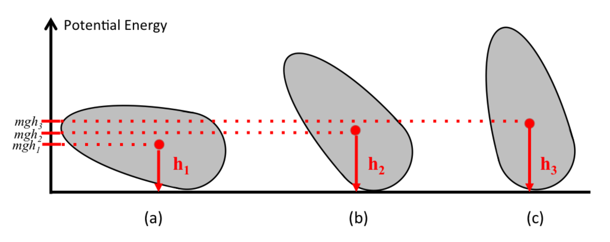
1.2. Curvature-Driven Model
2. Methods
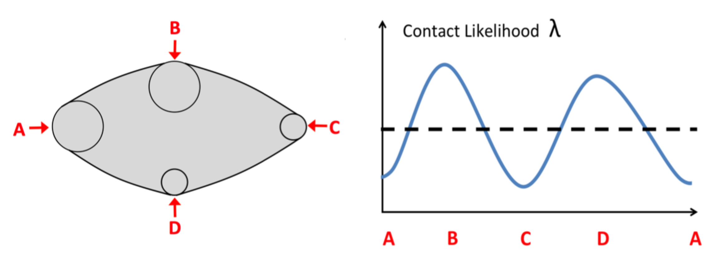
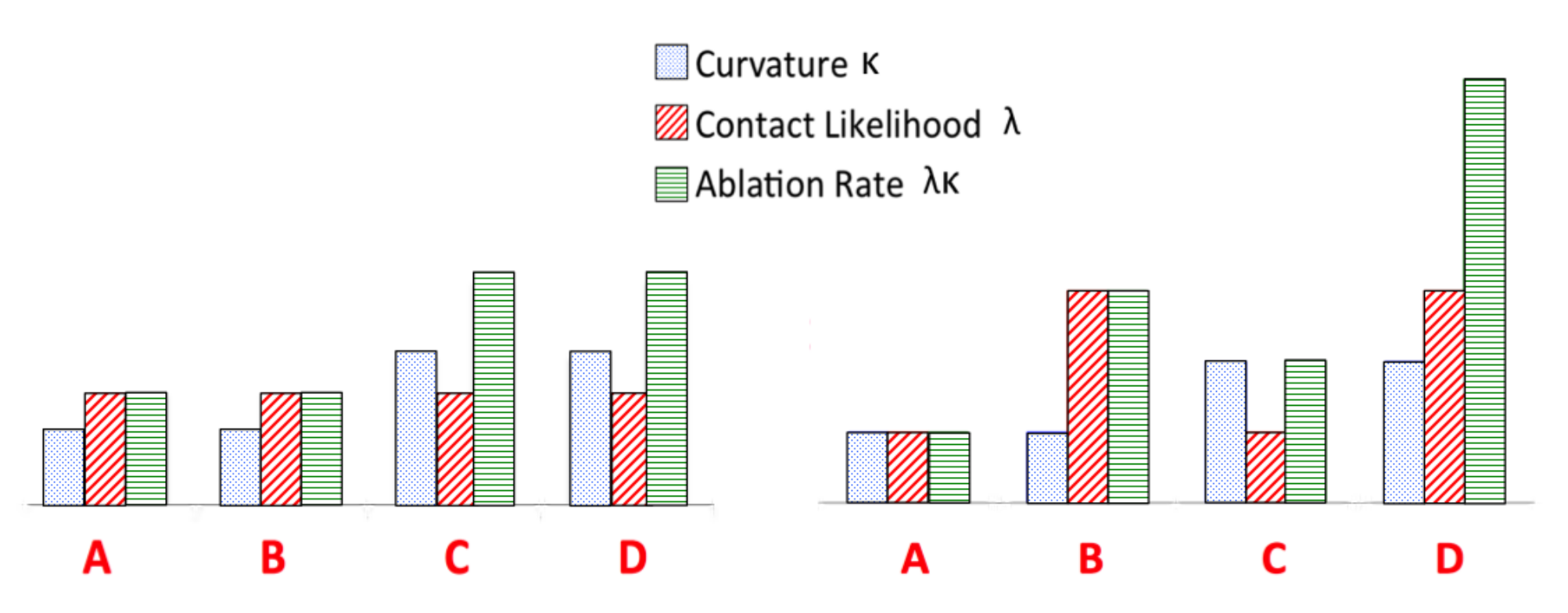
2.1. Curvature and Contact-Likelihood Model
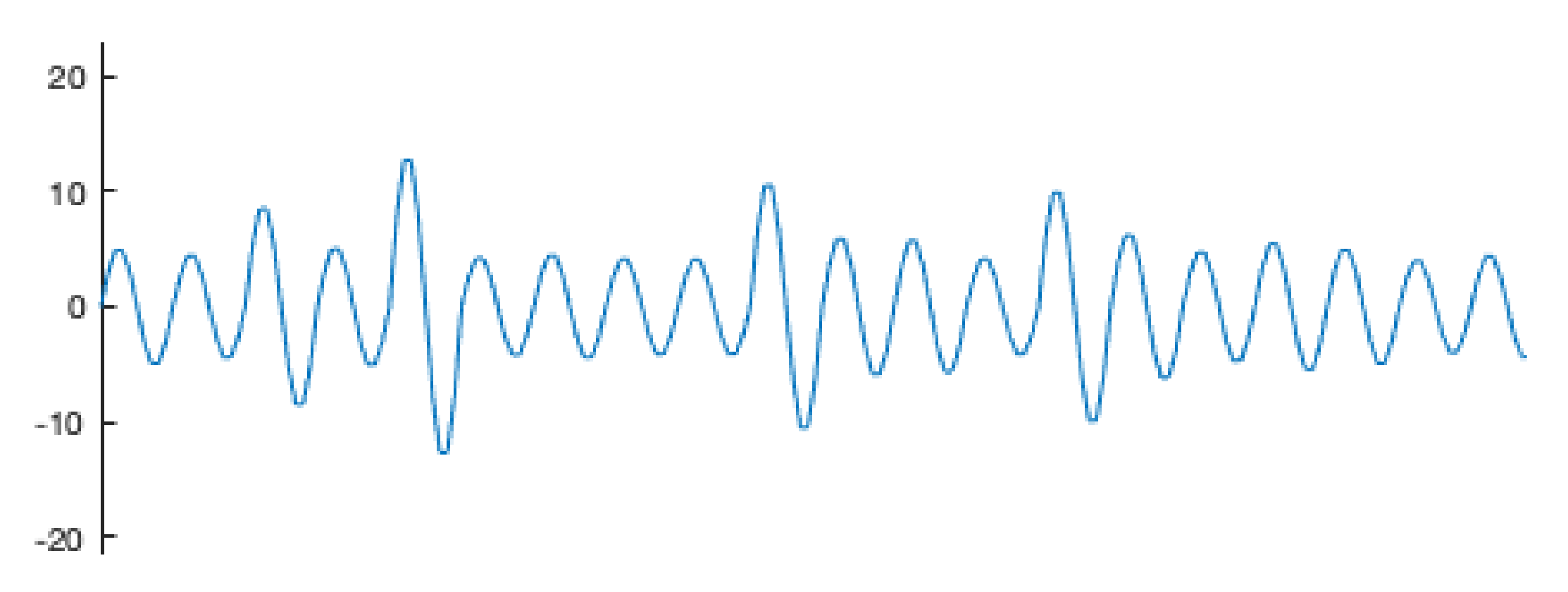
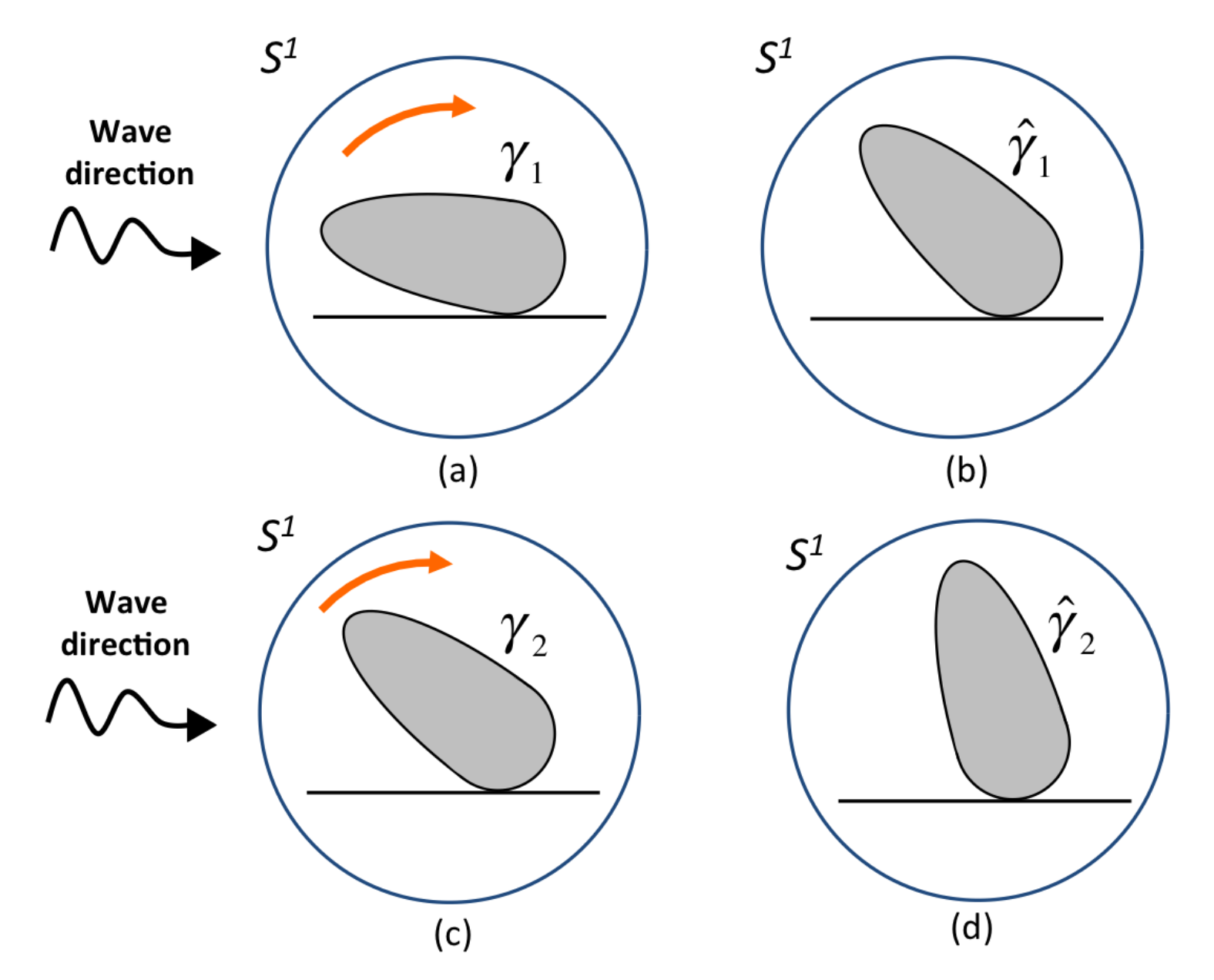
2.2. Wave Dynamics
2.3. Wave Steady-State Assumption
2.4. Contact-Likelihood Functions
2.4.1. Continuous Contact-Likelihood Functions
2.4.2. Discrete Contact-Likelihood Functions
3. A Prototypical Non-Isotropic Model under Pareto Wave Distribution
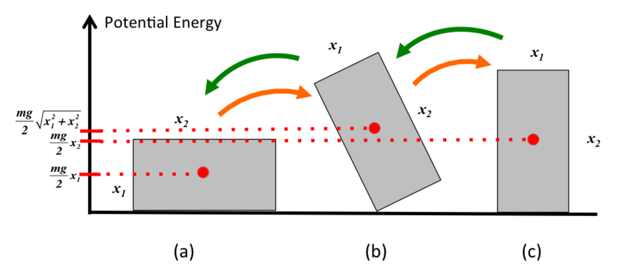
3.1. Thought Experiment for Equation (11)
3.2. Limiting Shapes
4. Preliminary Numerical Experiments
5. Discussion
Future Research Directions
- Prove or disprove that in the 2-d version of Aristotle’s Equation (1) with , for all convex initial shapes, the renormalized shapes converge to a circle for all and remain the same for . Determine the limiting renormalized shapes for , and for all for which there is convergence, identify the rates of convergence.
- Prove or disprove that besides the circle, there is only one simple closed solution to the 2-d equation when the sizes are renormalized; identify the equation for the non-circular solution if there is one. Prove or disprove that the circle is in unstable equilibrium and that the other simple closed solution is in stable equilibrium. More generally, do the same for solutions of Equation (11) for .
- Prove or disprove that besides the circle, there is only one simple closed solution to the 2-d equation ; identify the equation for the non-circular solution if there is one. More generally, do the same for for .
- Identify the equation for the unique (modulo rotations) simple closed non-circular solution to Berger’s 2-d equation (where r is the radius in polar coordinates), the existence of which is proved in [44]. More generally, do the same for for all .
- Prove or disprove that when the sizes (areas) are renormalized, the 2-d “stochastic slicing” process illustrated in Figure 19 converges in distribution, and if it converges, identify the limiting distribution and the rate of convergence.
- Prove or disprove that there is exactly one (modulo rotations) non-circular simple closed solution to (15) for , and that this interval is sharp.
- Extend all of the above to the 3-d setting and by replacing h by . (Same for the 3-d process in Figure 20).
- Perform detailed numerical analysis (e.g., using standard finite element methods) of the non-linear and non-local partial integro-differential equations (3) and (11), in both 2-d and 3-d, for various values of lambda and alpha. Present the results of this analysis in both tabular and graphical forms.
Supplementary Materials
Funding
Institutional Review Board Statement
Informed Consent Statement
Data Availability Statement
Acknowledgments
Conflicts of Interest
Appendix A. Pseudocode for Numerical Figures
- Fix a period
- Generate independent Pareto values with mean 2.
- Generate standard sin wave values.
- For the jth period, multiply by .
- Matlab code: may2waves.m
- Set S = an ellipse with minor axis 0.7, major axis 1, centered at the origin.
- START
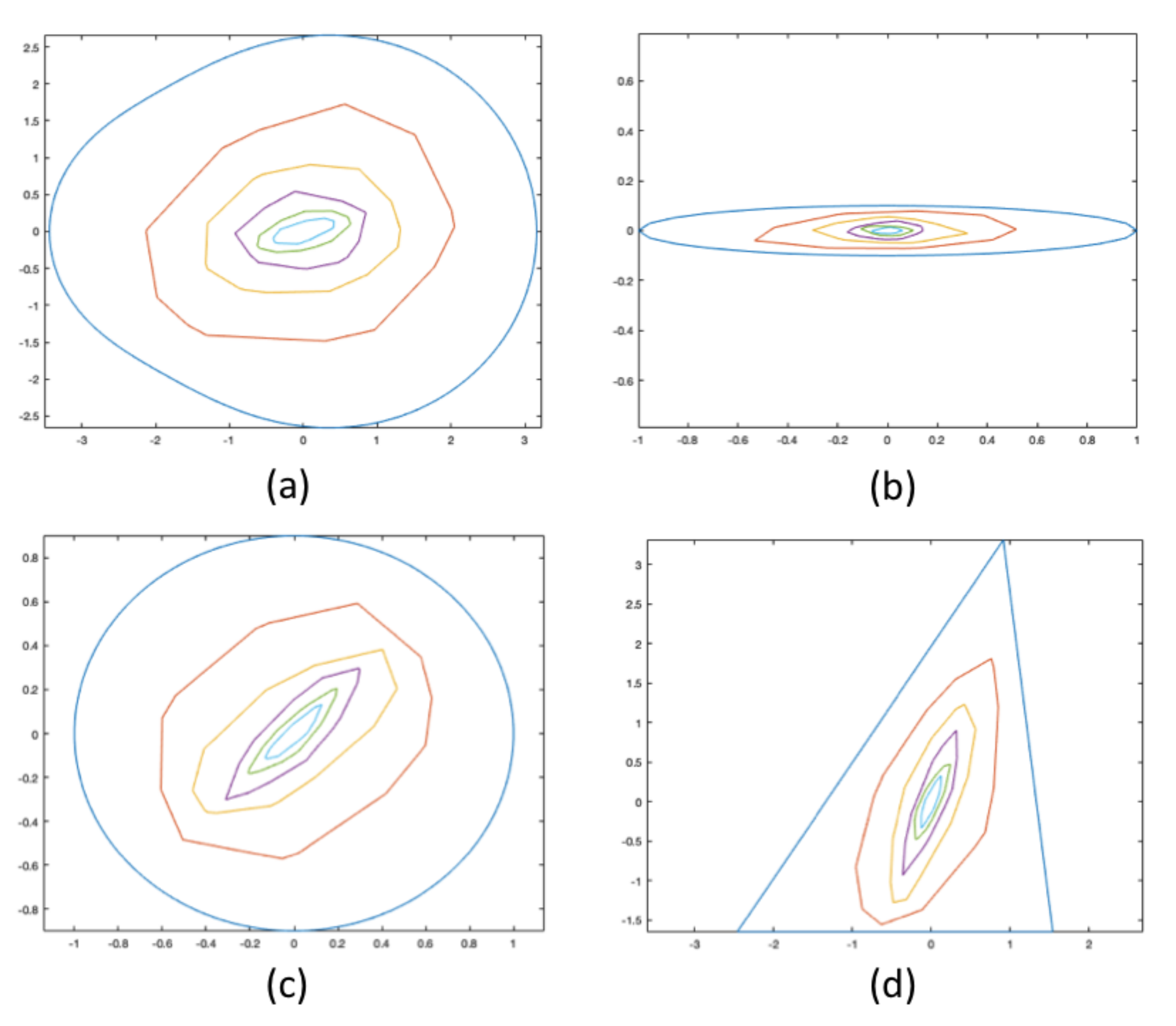
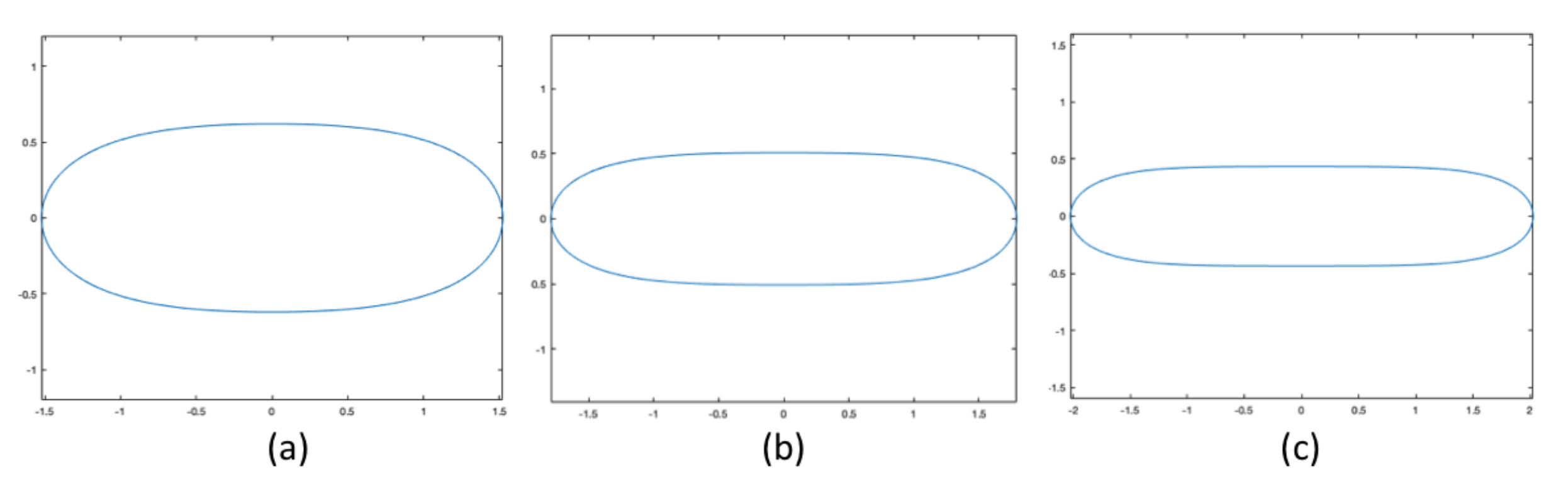
- Compute incremental new shape using a semi-implicit finite difference scheme for curve-shortening of S (with no tangential motion) under , where is a variable input to the program: 2.5 for (a), 3 for (b), and 4 for (c).
- Resize the shape to retain the same area.
- STOP IF all coordinates of the current shape differ from all coordinates of the previous by less than , i.e., the limiting shape of this equation has been reached.
- Set , return to START.
- Matlab code: Numerical_Solve_Curve_2.m
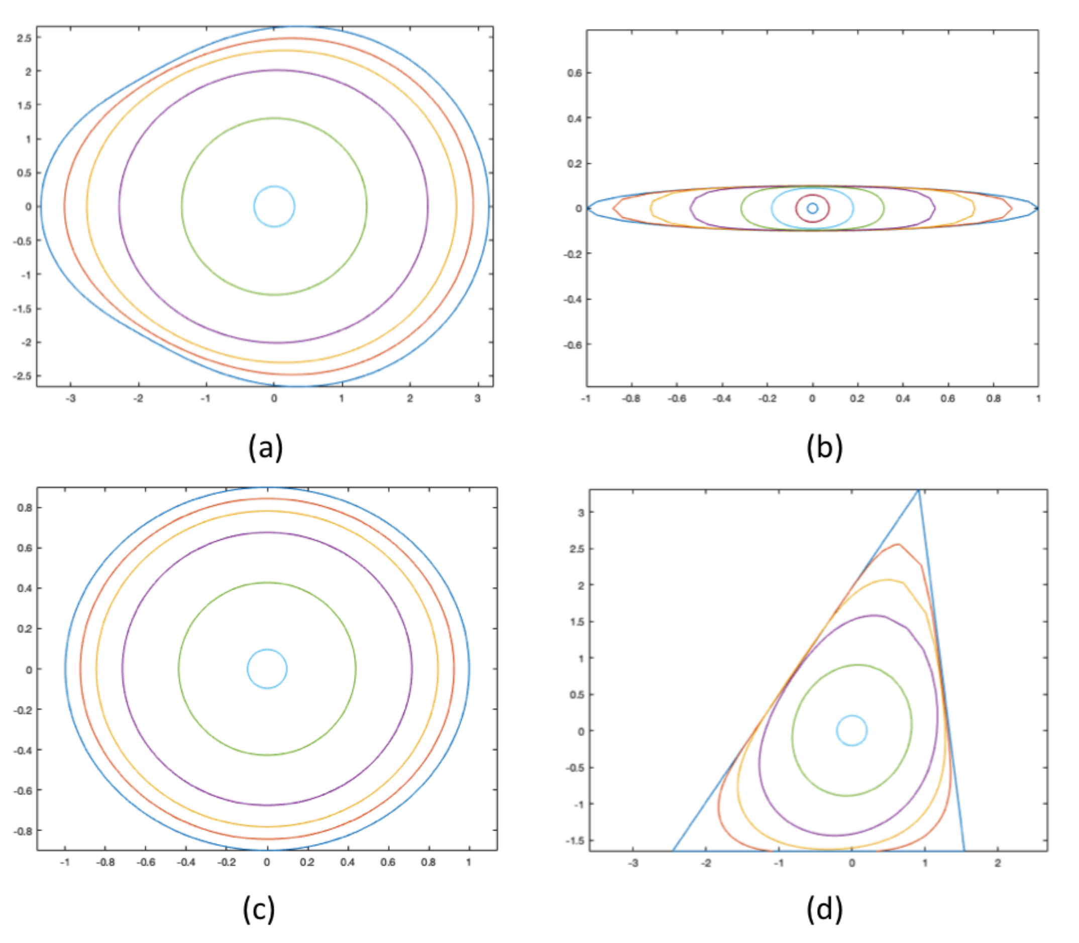
- START
- Calculate the center of mass of S.
- Compute incremental new shape using a stable explicit scheme (no tangential motion) for curve-shortening of S under , where h is the support function of S with as origin.
- Set , return to START.
- Matlab code: Aristotle.m
- Fix the origin O, and center all the stones so that center of mass is O.
- START
- Compute incremental new shape using a semi-implicit finite difference scheme for curve-shortening of S under , where h is the support function of S with origin at O. [Note: this scheme takes a , closed, embedded plane curve and deforms it for the life of the flow.]
- Set , return to START.
- Matlab code: New_CSF_Semi_Implicit_6.m
- Same as Figure 16 except using
- Matlab code: New_CSF_Semi_Implicit_6.m
- START
- Calculate the center of mass and the area of S.
- Shift the shape so that its center is at the origin.
- Generate a random angle uniformly in , and let .
- Choose an angle at random among the inversely proportional to , where h is the support function of S with origin at (0, 0).
- Compute distance d of the line perpendicular to , in the direction of from , so that it cuts off 0.01.
- Compute new shape after this cut.
- Set , return to START.
- Matlab code: DiscretizedStones.m
- First, produce the initial shape. We do this by denoting all vertices of the polygon, and then creating a mesh-grid out of those vertices (library does this by finding the convex shape with vertices, faces). For the eggshape and ellipsoid, we pass in the spherical coordinates and allow the function to create the mesh-grid. For the trapezoid, we use a library function and immediately pass in the mesh-grid values.
- Calculate the original volume
- Initialize xyz-coordinates of 12 equally spaced points, chosen as vertices of the icosahedron.
- START
- Center the shape
- Create a random 3-d rotation of the 12 vertices, using the yaw, pitch, and roll rotation matrices
- Calculate the distance h to the polygon surface in these 12 directions, and choose a direction with probability proportional to .
- If deterministic, move cuts along this direction incrementally, stopping when a perpendicular plane cuts away delta*volume_of_shape on the previous iteration. If random, choose a distance uniformly. Inspect the perpendicular cut made at this distance along the chosen direction. Accept this cut with probability exponentially decreasing in volume cut away, proportioned so that the average ratio of volume cut is delta.
- Determine the new volume, return to START.
- Matlab code: PolygonSlicing3D.m
- Same as Figure 14, except S = an ellipse with minor axis 0.5, major axis 1, and expNum = 2.2.
- Matlab code: Numerical_Solve_Curve_2.m
References
- Dobkins, J.E., Jr.; Folk, R.L. Shape Development On Tahiti-Nui. J. Sediment. Res. 1970, 40, 1167–1203. [Google Scholar] [CrossRef]
- Aristotle. Mechanica. In The Oxford Translation of the Complete Works of Aristotle; Ross, W.D., Ed.; Clarendon Press: Oxford, UK, 1913; Volume 6. [Google Scholar]
- Krynine, P.D. On the Antiquity of “Sedimentation" and Hydrology (with Some Moral Conclusions). Geol. Soc. Am. Bull. 1960, 71, 1721–1726. [Google Scholar] [CrossRef]
- Ashcroft, W. Beach pebbles explained. Nature 1990, 346, 227. [Google Scholar] [CrossRef]
- Black, W.T. On rolled pebbles from the beach at Dunbar. Trans. Edinb. Geol. Soc. 1877, 3, 122–123. [Google Scholar] [CrossRef]
- Bluck, B.J. Sedimentation of Beach Gravels: Examples from South Wales. J. Sediment. Res. 1967, 37, 128–156. [Google Scholar] [CrossRef]
- Carr, A.P. Size Grading Along A Pebble Beach: Chesil Beach, England. J. Sediment. Res. 1969, 39, 297–311. [Google Scholar] [CrossRef]
- Domokos, G.; Gibbons, G.W. The Geometry of Abrasion. In New Trends in Intuitive Geometry; Ambrus, G., Bárány, I., Böröczky, K.J., Tóth, G.F., Pach, J., Eds.; János Bolyai Mathematical Society: Budapest, Hungary; Springer: Cham, Switzerland, 2018; Volume 27, pp. 125–153. [Google Scholar] [CrossRef]
- Durian, D.J.; Bideaud, H.; Duringer, P.; Schröder, A.; Thalmann, F.; Marques, C.M. What Is in a Pebble Shape? Phys. Rev. Lett. 2006, 97, 028001. [Google Scholar] [CrossRef] [PubMed] [Green Version]
- Hamilton, R.S. Worn stones with flat sides. Discourses Math. Appl. 1994, 3, 69–78. [Google Scholar]
- Landon, R.E. An Analysis of Beach Pebble Abrasion and Transportation. J. Geol. 1930, 38, 437–446. [Google Scholar] [CrossRef]
- Lorang, M.S.; Komar, P.D. Pebble shape. Nature 1990, 347, 433–434. [Google Scholar] [CrossRef]
- Strutt, R.J. The ultimate shape of pebbles, natural and artificial. Proc. Math. Phys. Eng. Sci. 1942, 181, 107–118. [Google Scholar] [CrossRef] [Green Version]
- Wald, Q.R. The form of pebbles. Nature 1990, 345, 211. [Google Scholar] [CrossRef]
- Williams, A.T.; Caldwell, N.E. Particle size and shape in pebble-beach sedimentation. Mar. Geol. 1988, 82, 199–215. [Google Scholar] [CrossRef]
- Winzer, K. On the formation of elliptic stones due to periodic water waves. Eur. Phys. J. B 2013, 86, 464. [Google Scholar] [CrossRef]
- Strutt, R.J. Pebbles, natural and artificial, Their shape under various conditions of abrasion. Proc. Math. Phys. Eng. Sci. 1944, 182, 321–335. [Google Scholar] [CrossRef] [Green Version]
- Domokos, G.; Gibbons, G.W. The evolution of pebble size and shape in space and time. Proc. Math. Phys. Eng. Sci. 2012, 468, 3059–3079. [Google Scholar] [CrossRef]
- Kavallaris, N.I.; Suzuki, T. Non-Local Partial Differential Equations for Engineering and Biology; Springer International Publishing: Cham, Switzerland, 2018. [Google Scholar] [CrossRef]
- Firey, W.J. Shapes of worn stones. Mathematika 1974, 21, 1–11. [Google Scholar] [CrossRef]
- Fehér, E.; Domokos, G.; Krasukopf, B. Computing critical point evolution under planar curvature flows. arXiv 2020, arXiv:2010.11169. [Google Scholar]
- Andrews, B. Gauss curvature flow: The fate of the rolling stones. Invent. Math. 1999, 138, 151–161. [Google Scholar] [CrossRef]
- Andrews, B.; McCoy, J.; Zheng, Y. Contracting convex hypersurfaces by curvature. Calc. Var. Partial Differ. Equ. 2013, 47, 611–665. [Google Scholar] [CrossRef]
- Bloore, F.J. The shape of pebbles. J. Int. Assoc. Math. Geol. 1977, 9, 113–122. [Google Scholar] [CrossRef]
- Gage, M.E. Curve shortening makes convex curves circular. Invent. Math. 1984, 76, 357–364. [Google Scholar] [CrossRef]
- Strutt, R.J. Pebbles of regular shape and their production in experiment. Nature 1944, 154, 169–171. [Google Scholar] [CrossRef] [Green Version]
- Sipos, A.A.; Domokos, G.; Jerolmack, D.J. Shape evolution of ooids: A geometric model. Sci. Rep. 2018, 8, 1758. [Google Scholar] [CrossRef] [PubMed] [Green Version]
- Andrews, B. Evolving convex curves. Calc. Var. Partial Differ. Equ. 1998, 7, 315–371. [Google Scholar] [CrossRef]
- Andrews, B. Classification of limiting shapes for isotropic curve flows. J. Am. Math. Soc. 2002, 16, 443–459. [Google Scholar] [CrossRef] [Green Version]
- Ghosh, P.K.; Kumar, K.V. Support Function Representation of Convex Bodies, Its Application in Geometric Computing, and Some Related Representations. Comput. Vis. Image Underst. 1998, 72, 379–403. [Google Scholar] [CrossRef] [Green Version]
- Geman, D.; Horowitz, J. Occupation Densities. Ann. Probab. 1980, 8, 1–67. [Google Scholar] [CrossRef]
- Chen, B.Y.; Zhang, K.Y.; Wang, L.P.; Jiang, S.; Liu, G.L. Generalized Extreme Value-Pareto Distribution Function and Its Applications in Ocean Engineering. China Ocean Eng. 2019, 33, 127–136. [Google Scholar] [CrossRef]
- Mackay, E.B.L.; Challenor, P.G.; Bahaj, A.S. A comparison of estimators for the generalised Pareto distribution. Ocean Eng. 2011, 38, 1338–1346. [Google Scholar] [CrossRef]
- Stansell, P. Distributions of extreme wave, crest and trough heights measured in the North Sea. Ocean Eng. 2005, 32, 1015–1036. [Google Scholar] [CrossRef]
- Teixeira, R.; Nogal, M.; O’Connor, A. On the suitability of the generalized Pareto to model extreme waves. J. Hydraul. Res. 2018, 56, 755–770. [Google Scholar] [CrossRef] [Green Version]
- Winzer, K. The temporal formation and the shape of ellipsoidal stones on the beaches of the oceans. Eur. Phys. J. Plus 2017, 132, 443. [Google Scholar] [CrossRef]
- Björk, T. The Pedestrian’s Guide to Local Time. arXiv 2015, arXiv:1512.08912. [Google Scholar]
- Deckelnick, K.; Dziuk, G. On the approximation of the curve shortening flow. In Calculus of Variations, Applications and Computations; Bandle, C., Chipot, M., Paulin, J.S.J., Bemelmans, J., Shafrir, I., Eds.; Longman Scientific & Technical: Essex, UK, 1994; pp. 100–108. [Google Scholar]
- Domokos, G.; Sipos, A.Á.; Várkonyi, P.L. Countinuous and discrete models for abrasion processes. Period. Polytech. Archit. 2009, 40, 3–8. [Google Scholar] [CrossRef]
- Krapivsky, P.L.; Redner, S. Smoothing a rock by chipping. Phys. Rev. E 2007, 75, 031119. [Google Scholar] [CrossRef] [PubMed] [Green Version]
- Priour, D.J., Jr. Time Scales for Rounding of Rocks through Stochastic Chipping. arXiv 2020, arXiv:2003.03476. [Google Scholar]
- Gowers, T. Mathematics: A Very Short Introduction; Oxford University Press: Oxford, UK, 2002. [Google Scholar]
- Sipos, A.A.; Domokos, G.; Török, J. Particle size dynamics in abrading pebble populations. Earth Surf. Dyn. 2021, 9, 235–251. [Google Scholar] [CrossRef]
- Berger, A. On planar curves with position-dependent curvature. arXiv 2021, arXiv:2107.07680. [Google Scholar]


Publisher’s Note: MDPI stays neutral with regard to jurisdictional claims in published maps and institutional affiliations. |
© 2022 by the author. Licensee MDPI, Basel, Switzerland. This article is an open access article distributed under the terms and conditions of the Creative Commons Attribution (CC BY) license (https://creativecommons.org/licenses/by/4.0/).
Share and Cite
Hill, T.P. On the Oval Shapes of Beach Stones. AppliedMath 2022, 2, 16-38. https://doi.org/10.3390/appliedmath2010002
Hill TP. On the Oval Shapes of Beach Stones. AppliedMath. 2022; 2(1):16-38. https://doi.org/10.3390/appliedmath2010002
Chicago/Turabian StyleHill, Theodore P. 2022. "On the Oval Shapes of Beach Stones" AppliedMath 2, no. 1: 16-38. https://doi.org/10.3390/appliedmath2010002
APA StyleHill, T. P. (2022). On the Oval Shapes of Beach Stones. AppliedMath, 2(1), 16-38. https://doi.org/10.3390/appliedmath2010002