
Extreme Value Analysis of Ocean Still Water Levels along the USA East Coast—Case Study (Key West, Florida)


Abstract
:1. Introduction
- high-intensity dynamic component (comprising the limit of any hurricane driven storm surge above the coincident tide condition);
- the prevailing tide coupled with any other omnipresent anomalies driven by prevailing oceanographic effects; and
- coincident, long timescale rise in relative MSL (due principally to climate change drivers and vertical land motion influences).
2. Materials and Methods
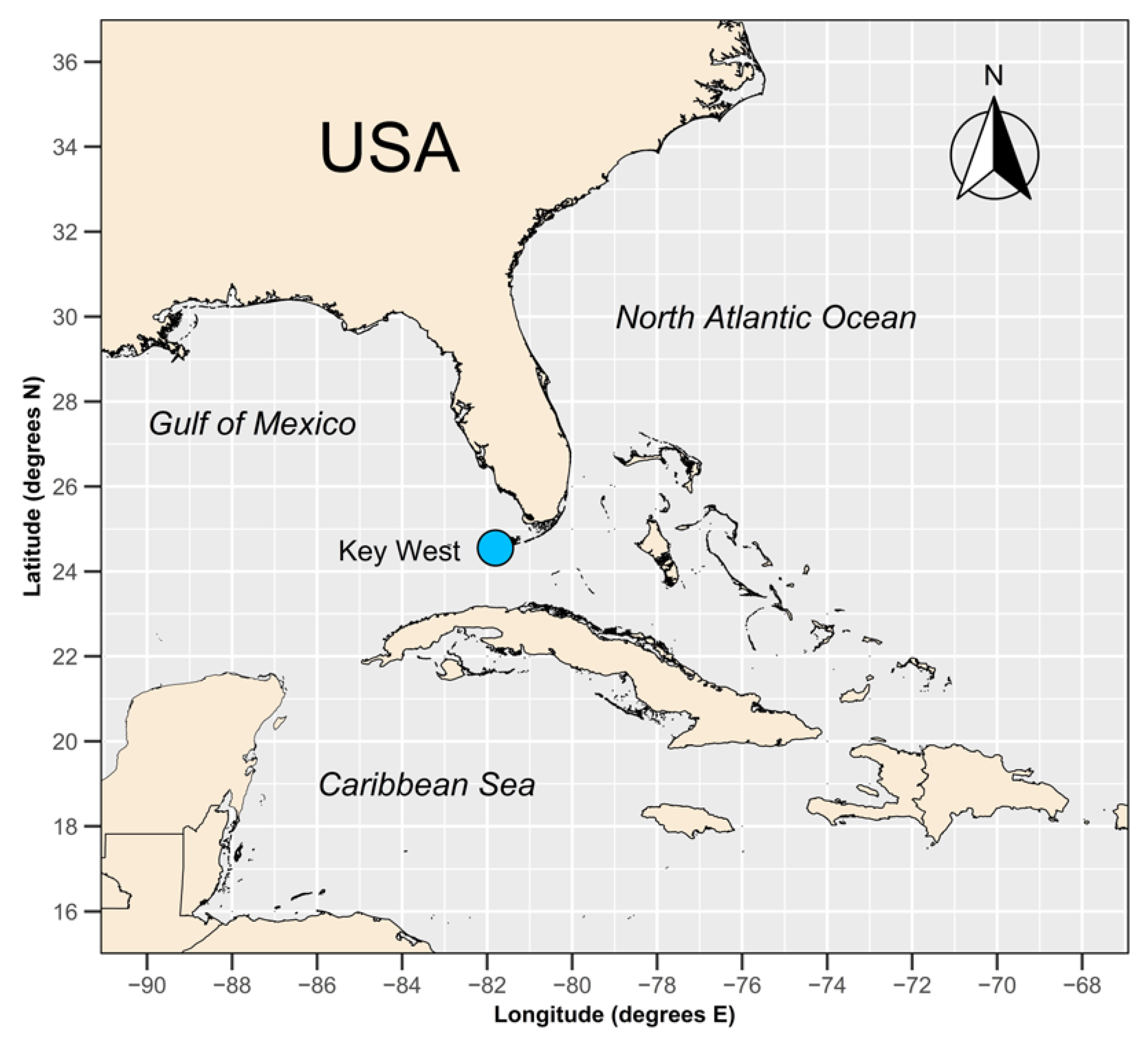
2.1. Data Sources Used in the Study
2.2. Methodology
3. Results
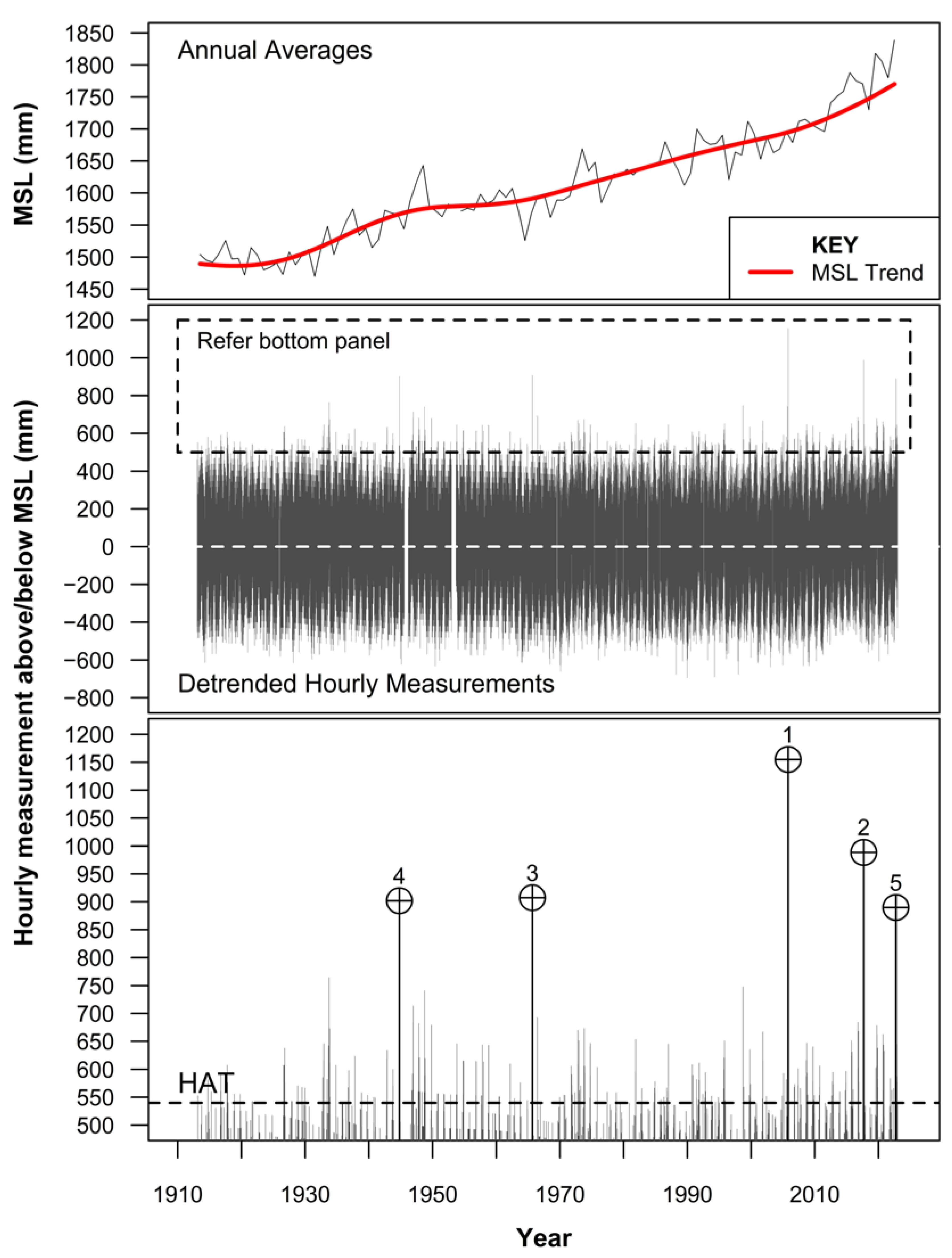
3.1. Hourly Tide Gauge Record
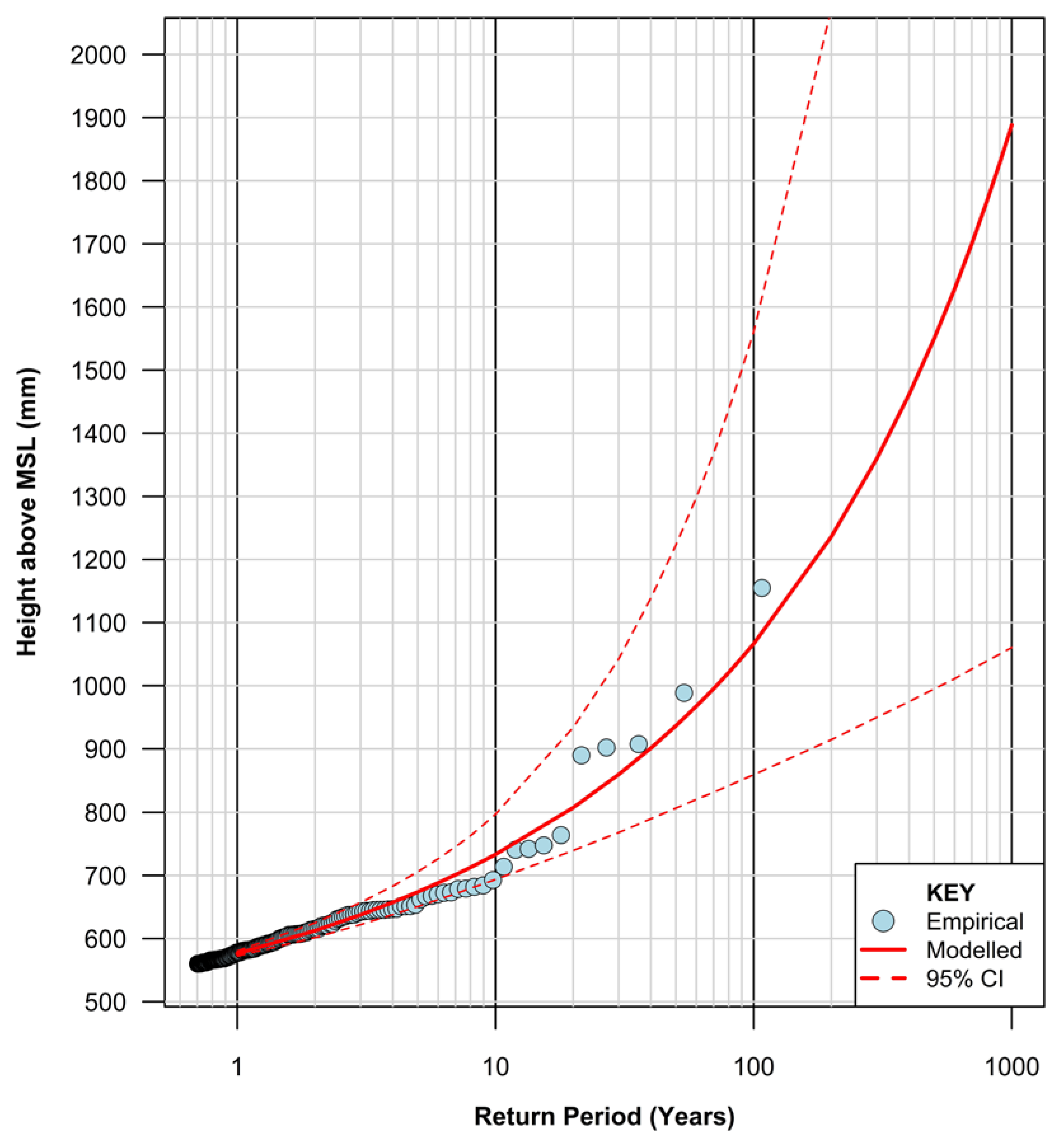
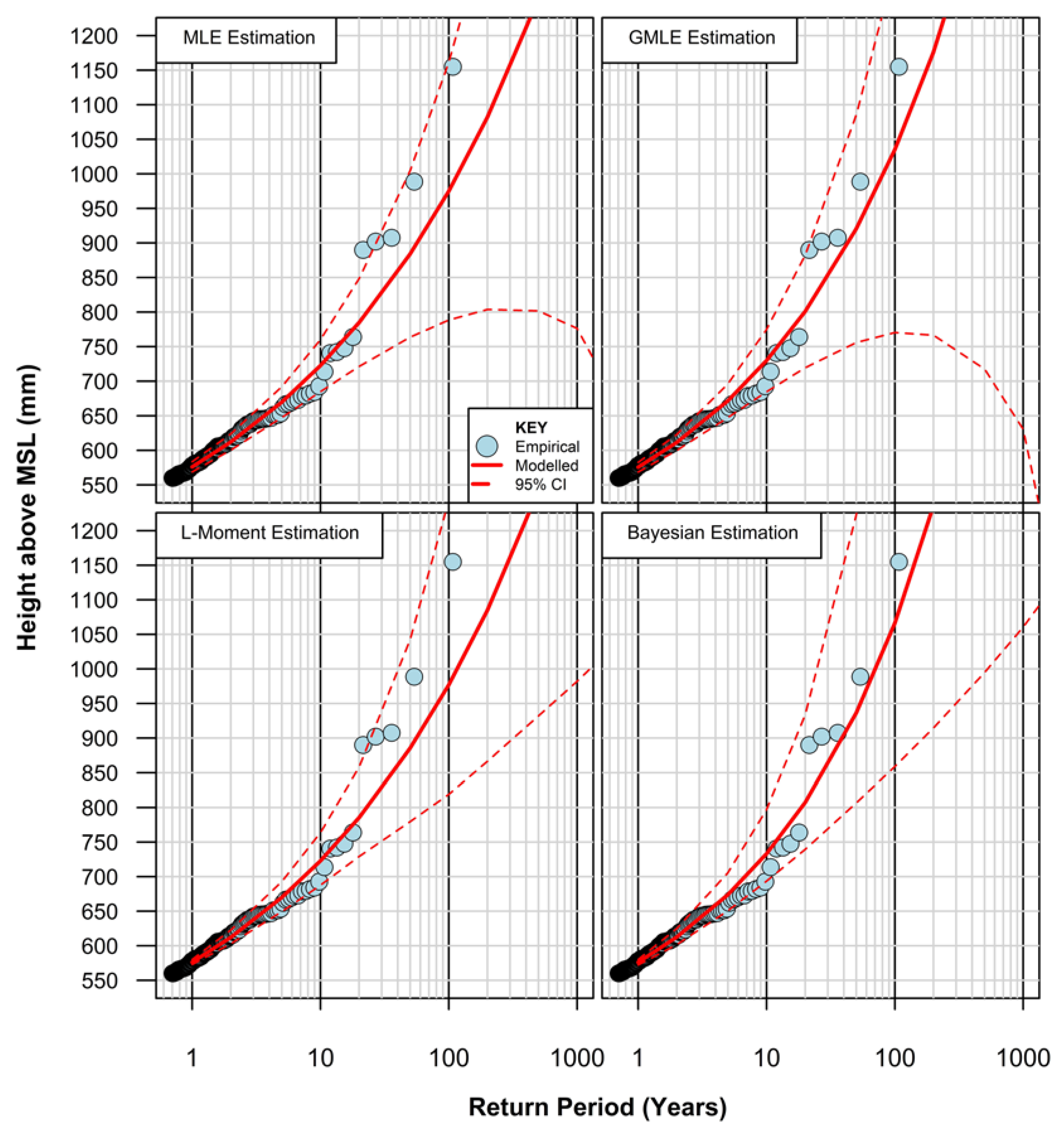
3.2. Extreme Value Analysis
4. Discussion
4.1. Is There Any Evidence to Suggest Extremes Have Been Increasing over Time?
4.2. Sensitivity Analysis Testing for EVA
4.3. The Shape of the EVA Return Level Plot
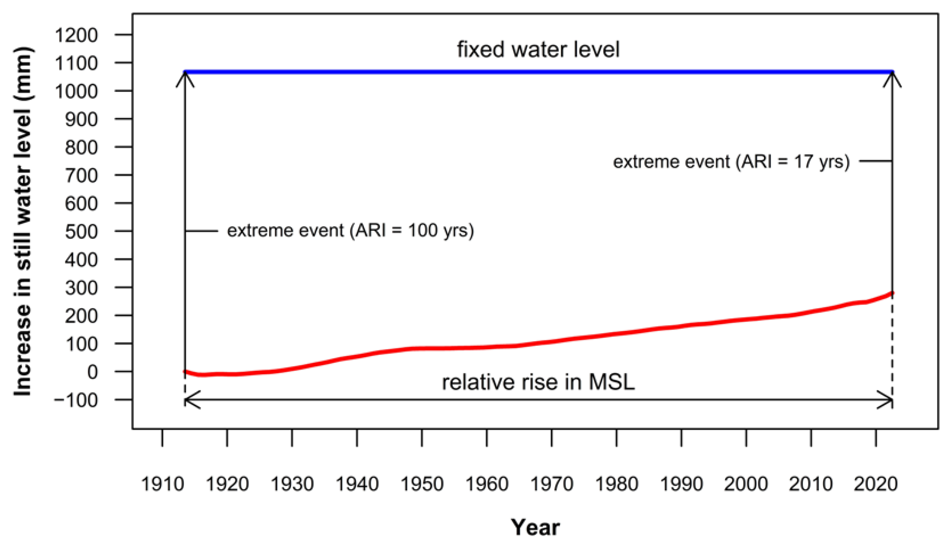
4.4. Influence of Future Sea Level Projections on Predictions of Extreme Water Levels
4.5. Recommendations for EVA Applied to Ocean Water Level Records
- use hourly, quality controlled tide gauge data;
- detrend and decluster the hourly data inputs (to attain stationarity and independence requirements for EVA);
- apply the POT approach with the GPD model fit;
- threshold selection recommended above HAT;
- optimize threshold selection through the use of tools such as mean excess plot;
- test a range of thresholds to better understand key sensitivities (if necessary);
- use Bayesian method to optimize parameter estimation; and
- confirm optimum threshold and parameter estimation method through visual diagnostic means including return level plots and Q-Q plots to observe the performance of the model fit within uncertainty bounds to the more extreme values.
4.6. Limitations of the Analysis and Results
5. Conclusions
Funding
Institutional Review Board Statement
Informed Consent Statement
Data Availability Statement
Acknowledgments
Conflicts of Interest
References
- IPCC; Masson-Delmotte, V.; Zhai, P.; Pirani, A.; Connors, S.L.; Péan, C.; Berger, S.; Caud, N.; Chen, Y.; Goldfarb, L.; et al. Climate Change 2021: The Physical Science Basis; Contribution of Working Group I to the Sixth Assessment Report of the Intergovernmental Panel on Climate Change; Cambridge University Press: Cambridge, UK; New York, NY, USA, 2021. [Google Scholar]
- Reidmiller, D.R.; Avery, C.W.; Easterling, D.R.; Kunkel, K.E.; Lewis, K.L.M.; Maycock, T.K.; Stewart, B.C. (Eds.) Impacts, Risks, and Adaptation in the United States: Fourth National Climate Assessment (NCA4); U.S. Global Change Research Program: Washington, DC, USA, 2018; Volume II.
- Fleming, E.; Craghan, M.; Haines, J.; Finzi Hart, J.; Stiller, H.; Sutton-Grier, A. Coastal Effects. In Impacts, Risks, and Adaptation in the United States: Fourth National Climate Assessment, Volume II; Reidmiller, D.R., Avery, C.W., Easterling, D.R., Kunkel, K.E., Lewis, K.L.M., Maycock, T.K., Stewart, B.C., Eds.; U.S. Global Change Research Program: Washington, DC, USA, 2018; pp. 322–352. [Google Scholar]
- Garner, A.J.; Sosa, S.E.; Tan, F.; Tan, C.W.J.; Garner, G.G.; Horton, B.P. Evaluating Knowledge Gaps in Sea-Level Rise Assessments From the United States. Earths Future 2023, 11, e2022EF003187. [Google Scholar] [CrossRef]
- Fu, X.; Sun, B.; Frank, K.; Peng, Z.-R. Evaluating Sea-Level Rise Vulnerability Assessments in the USA. Clim. Chang. 2019, 155, 393–415. [Google Scholar] [CrossRef]
- Watson, P.J. Status of Mean Sea Level Rise around the USA (2020). GeoHazards 2021, 2, 80–100. [Google Scholar] [CrossRef]
- Hauer, M.E.; Hardy, D.; Kulp, S.A.; Mueller, V.; Wrathall, D.J.; Clark, P.U. Assessing Population Exposure to Coastal Flooding Due to Sea Level Rise. Nat. Commun. 2021, 12, 6900. [Google Scholar] [CrossRef]
- Sweet, W.V.; Hamlington, B.D.; Kopp, R.E.; Weaver, C.P.; Barnard, P.L.; Bekaert, D.; Brooks, W.; Craghan, M.; Dusek, G.; Frederikse, T.; et al. Global and Regional Sea Level Rise Scenarios for the United States: Updated Mean Projections and Extreme Water Level Probabilities Along U.S. Coastlines; NOAA Technical Report NOS 01; National Oceanic and Atmospheric Administration: Washington, DC, USA; National Ocean Service: Silver Spring, MD, USA, 2022.
- Annual Assessment of Flooding and Sea Level Rise, 2022 ed.; Office of Economic and Demographic Research (EDR), The Florida Legislature: Tallahassee, FL, USA, 2022; Volume 4.
- Parkinson, R.W.; Harlem, P.W.; Meeder, J.F. Managing the Anthropocene Marine Transgression to the Year 2100 and beyond in the State of Florida U.S.A. Clim. Chang. 2015, 128, 85–98. [Google Scholar] [CrossRef]
- Watson, P.J. Determining Extreme Still Water Levels for Design and Planning Purposes Incorporating Sea Level Rise: Sydney, Australia. Atmosphere 2022, 13, 95. [Google Scholar] [CrossRef]
- Coles, S. An Introduction to Statistical Modeling of Extreme Values; Springer: London, UK, 2001; ISBN 978-1-84996-874-4. [Google Scholar]
- Embrechts, P.; Klüppelberg, C.; Mikosch, T. Modelling Extremal Events; Springer: Berlin/Heidelberg, Germany, 1997; ISBN 978-3-642-08242-9. [Google Scholar]
- Teena, N.V.; Sanil Kumar, V.; Sudheesh, K.; Sajeev, R. Statistical Analysis on Extreme Wave Height. Nat. Hazards 2012, 64, 223–236. [Google Scholar] [CrossRef]
- Abild, J.; Andersen, E.Y.; Rosbjerg, D. The Climate of Extreme Winds at the Great Belt, Denmark. J. Wind Eng. Ind. Aerodyn. 1992, 41, 521–532. [Google Scholar] [CrossRef]
- Dupuis, D.J. Exceedances over High Thresholds: A Guide to Threshold Selection. Extremes 1999, 1, 251–261. [Google Scholar] [CrossRef]
- Arns, A.; Wahl, T.; Haigh, I.D.; Jensen, J.; Pattiaratchi, C. Estimating Extreme Water Level Probabilities: A Comparison of the Direct Methods and Recommendations for Best Practise. Coast. Eng. 2013, 81, 51–66. [Google Scholar] [CrossRef]
- Caires, S. Extreme Value Analysis: Wave Data; World Meteorological Organization: Geneva, Switzerland, 2011. [Google Scholar]
- R Development Core Team R: A Language and Environment for Statistical Computing; R Foundation for Statistical Computing: Vienna, Austria, 2021.
- Gilleland, E.; Katz, R.W. ExtRemes 2.0: An Extreme Value Analysis Package in R. J. Stat. Softw. 2016, 72, 1–39. [Google Scholar] [CrossRef]
- PSMSL Permanent Service for Mean Sea Level. Available online: https://www.psmsl.org/data/obtaining/ (accessed on 21 September 2021).
- Holgate, S.J.; Matthews, A.; Woodworth, P.L.; Rickards, L.J.; Tamisiea, M.E.; Bradshaw, E.; Foden, P.R.; Gordon, K.M.; Jevrejeva, S.; Pugh, J. New Data Systems and Products at the Permanent Service for Mean Sea Level. J. Coast. Res. 2013, 29, 493–504. [Google Scholar] [CrossRef]
- UHSLC University of Hawaii Sea Level Centre. Available online: http://uhslc.soest.hawaii.edu/data/ (accessed on 1 March 2023).
- Caldwell, P.C.; Merrifield, M.A.; Thompson, P.R. Sea Level Measured by Tide Gauges from Global Oceans—The Joint Archive for Sea Level Holdings (NCEI Accession 0019568), version 5.5; NOAA National Centers for Environmental Information: Asheville, NC, USA, 2015.
- National Oceanic and Atmospheric Administration’s Center for Operational Oceano-Graphic Products and Services (CO-OPS). Available online: https://tidesandcurrents.noaa.gov/ (accessed on 1 March 2023).
- Fox-Kemper, B.; Hewitt, H.T.; Xiao, C.; Aðalgeirsdóttir, G.; Drijfhout, S.S.; Edwards, T.L.; Golledge, N.R.; Hemer, M.; Kopp, R.E.; Krinner, G.; et al. Ocean, Cryosphere and Sea Level Change. In Climate Change 2021: The Physical Science Basis. Contribution of Working Group I to the Sixth Assessment Report of the Intergovernmental Panel on Climate Change; Masson-Delmotte, V., Zhai, P., Pirani, A., Connors, S.L., Péan, C., Berger, S., Caud, N., Chen, Y., Goldfarb, L., Gomis, M.I., et al., Eds.; Cambridge University Press: Cambridge, UK; New York, NY, USA, 2021; pp. 1211–1362. [Google Scholar]
- Garner, G.G.; Kopp, R.E.; Hermans, T.; Slangen, A.B.A.; Edwards, T.L.; Levermann, A.; Nowikci, S.; Palmer, M.D.; Smith, C.; Fox-Kemper, B.; et al. IPCC AR6 Sea-Level Rise Projections, Version 20210809; PO.DAAC, CA, USA. 2021. Available online: https://zenodo.org/record/6382554 (accessed on 1 March 2023).
- Garner, G.G.; Kopp, R.E.; Hermans, T.; Slangen, A.B.A.; Koubbe, G.; Turilli, M.; Jha, S.; Edwards, T.L.; Levermann, A.; Nowikci, S.; et al. Framework for Assessing Changes to Sea-Level (FACTS) v1.0-rc: A Platform for Characterizing Parametric and Structural Uncertainty in Future Global, Relative, and Extreme Sea-Level Change. 2023. Available online: https://egusphere.copernicus.org/preprints/2023/egusphere-2023-14/ (accessed on 1 March 2023).
- National Oceanic and Atmospheric Administration National Hurricane Center. Available online: https://www.nhc.noaa.gov/data/#hurdat (accessed on 1 March 2023).
- Ramachandra Rao, A.; Hamed, K.H. (Eds.) Flood Frequency Analysis; CRC Press: Boca Raton, FL, USA, 2019; ISBN 9780429128813. [Google Scholar]
- Gumbel, E.J. Statistics of Extremes; Oxford University Press: Oxford, UK, 1958. [Google Scholar]
- Beirlant, J.; Goegebeur, Y.; Teugels, J.; Segers, J. Statistics of Extremes; John Wiley & Sons, Ltd.: Chichester, UK, 2004; ISBN 9780470012383. [Google Scholar]
- Pickands, J. Statistical Inference Using Extreme Order Statistics. Ann. Stat. 1975, 3, 119–131. [Google Scholar]
- Watson, P.J.; Lim, H.S. An Update on the Status of Mean Sea Level Rise around the Korean Peninsula. Atmosphere 2020, 11, 1153. [Google Scholar] [CrossRef]
- Watson, P.J. Identifying the Best Performing Time Series Analytics for Sea Level Research. In Time Series Analysis and Forecasting; Contributions to Statistics; Rojas, I., Pomares, H., Eds.; Springer: Cham, Switzerland, 2016; pp. 261–278. [Google Scholar]
- Watson, P.J. Improved Techniques to Estimate Mean Sea Level, Velocity and Acceleration from Long Ocean Water Level Time Series to Augment Sea Level (and Climate Change) Research; University of New South Wales: Sydney, Australia, 2018. [Google Scholar]
- Watson, P.J. Updated Mean Sea-Level Analysis: Australia. J. Coast. Res. 2020, 36, 915–931. [Google Scholar] [CrossRef]
- Kondrashov, D.; Ghil, M. Spatio-Temporal Filling of Missing Points in Geophysical Data Sets. Nonlinear Process Geophys. 2006, 13, 151–159. [Google Scholar] [CrossRef]
- Golyandina, N.; Korobeynikov, A.; Zhigljavsky, A. Singular Spectrum Analysis with R; Springer: Berlin/Heidelberg, Germany, 2018; ISBN 9783662573785. [Google Scholar]
- Watson, P.J. TrendSLR: Estimating Trend, Velocity and Acceleration from Sea Level Records. 2019. Available online: https://cran.r-project.org/web/packages/TrendSLR/index.html (accessed on 1 March 2023).
- Katz, R.W.; Parlange, M.B.; Naveau, P. Statistics of Extremes in Hydrology. Adv. Water Resour. 2002, 25, 1287–1304. [Google Scholar] [CrossRef]
- Ghosh, S.; Resnick, S. A Discussion on Mean Excess Plots. Stoch. Process. Appl. 2010, 120, 1492–1517. [Google Scholar] [CrossRef]
- Scarrott, C.; MacDonald, A. A Review of Extreme Value Threshold Estimation and Uncertainty Quantification. REVSTAT-Stat. J. 2012, 10, 33–60. [Google Scholar]
- Thompson, P.; Cai, Y.; Reeve, D.; Stander, J. Automated Threshold Selection Methods for Extreme Wave Analysis. Coast. Eng. 2009, 56, 1013–1021. [Google Scholar] [CrossRef]
- Davison, A.C.; Smith, R.L. Models for Exceedances Over High Thresholds. J. R. Stat. Soc. Ser. B (Methodol.) 1990, 52, 393–425. [Google Scholar] [CrossRef]
- Yılmaz, A.; Kara, M.; Özdemir, O. Comparison of Different Estimation Methods for Extreme Value Distribution. J. Appl. Stat. 2021, 48, 2259–2284. [Google Scholar] [CrossRef] [PubMed]
- City of Miami, Florida Website. Available online: https://www.miamigov.com/My-Government/ClimateChange/King-Tides (accessed on 9 March 2023).
- Reed, K.A.; Wehner, M.F.; Zarzycki, C.M. Attribution of 2020 Hurricane Season Extreme Rainfall to Human-Induced Climate Change. Nat. Commun. 2022, 13, 1905. [Google Scholar] [CrossRef] [PubMed]
- Camargo, S.J.; Giulivi, C.F.; Sobel, A.H.; Wing, A.A.; Kim, D.; Moon, Y.; Strong, J.D.O.; del Genio, A.D.; Kelley, M.; Murakami, H.; et al. Characteristics of Model Tropical Cyclone Climatology and the Large-Scale Environment. J. Clim. 2020, 33, 4463–4487. [Google Scholar] [CrossRef]
- Hawkes, P.J.; Gonzalez-Marco, D.; Sánchez-Arcilla, A.; Prinos, P. Best Practice for the Estimation of Extremes: A Review. J. Hydraul. Res. 2008, 46, 324–332. [Google Scholar] [CrossRef]
- Pasch, R.J.; Blake, E.S.; Cobb, H.D., III; Roberts, D.P. Tropical Cyclone Report Hurricane Wilma 15–25 October 2005. Available online: https://www.nhc.noaa.gov/data/tcr/AL252005_Wilma.pdf (accessed on 1 March 2023).


| Year | SSP1-1.9 | SSP1-2.6 | SSP2-4.5 | SSP3-7.0 | SSP5-8.5 |
|---|---|---|---|---|---|
| 2020 | 0 | 0 | 0 | 0 | 0 |
| 2030 | 43 | 43 | 44 | 45 | 48 |
| 2040 | 79 | 87 | 93 | 96 | 107 |
| 2050 | 127 | 140 | 155 | 166 | 182 |
| 2060 | 161 | 183 | 213 | 233 | 260 |
| 2070 | 211 | 241 | 281 | 317 | 354 |
| 2080 | 252 | 289 | 354 | 409 | 459 |
| 2090 | 299 | 337 | 427 | 512 | 583 |
| 2100 | 335 | 387 | 507 | 630 | 716 |
| 2110 | 379 | 448 | 579 | 709 | 806 |
| 2120 | 417 | 496 | 653 | 819 | 930 |
| 2130 | 453 | 542 | 726 | 929 | 1050 |
| 2140 | 487 | 588 | 799 | 1037 | 1164 |
| 2150 | 520 | 632 | 870 | 1141 | 1272 |
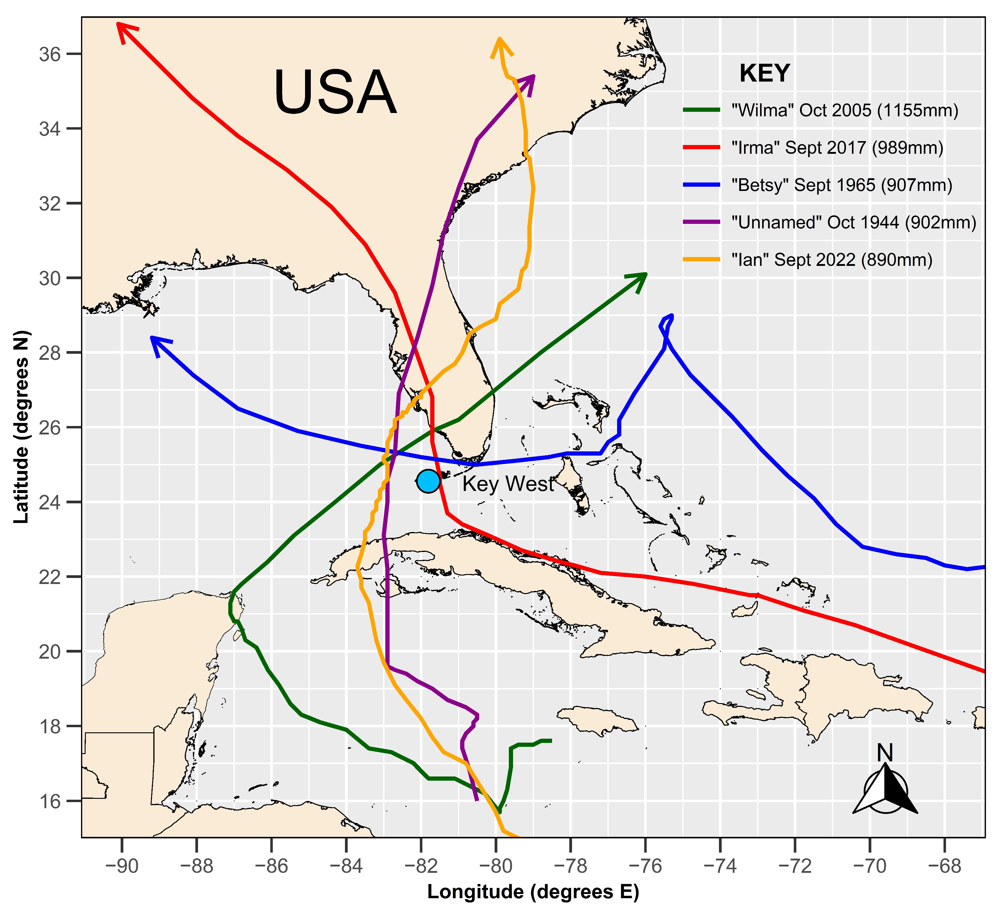
| Rank | Measurements above MSL (mm) 1 | Date (Time, hrs) | Hurricane Event 2 |
|---|---|---|---|
| 1 | 1155 | 24 October 2005 (0700) | Wilma |
| 2 | 989 | 10 September 2017 (1700) | Irma |
| 3 | 907 | 8 September 1965 (1400) | Betsy |
| 4 | 902 | 18 October 1944 (2200) | Unnamed |
| 5 | 890 | 28 September 2022 (0300) | Ian |
| 6 | 764 | 5 October 1933 (0300) | Unnamed |
| 7 | 748 | 25 September 1998 (1800) | Georges |
| 8 | 742 | 21 September 2005 (0200) | Rita |
| 9 | 741 | 21 September 1948 (1700) | Unnamed |
| 10 | 714 | 9 December 1946 (0700) | - |
Disclaimer/Publisher’s Note: The statements, opinions and data contained in all publications are solely those of the individual author(s) and contributor(s) and not of MDPI and/or the editor(s). MDPI and/or the editor(s) disclaim responsibility for any injury to people or property resulting from any ideas, methods, instructions or products referred to in the content. |
© 2023 by the author. Licensee MDPI, Basel, Switzerland. This article is an open access article distributed under the terms and conditions of the Creative Commons Attribution (CC BY) license (https://creativecommons.org/licenses/by/4.0/).
Share and Cite
Watson, P.J. Extreme Value Analysis of Ocean Still Water Levels along the USA East Coast—Case Study (Key West, Florida). Coasts 2023, 3, 294-312. https://doi.org/10.3390/coasts3040018
Watson PJ. Extreme Value Analysis of Ocean Still Water Levels along the USA East Coast—Case Study (Key West, Florida). Coasts. 2023; 3(4):294-312. https://doi.org/10.3390/coasts3040018
Chicago/Turabian StyleWatson, Phil J. 2023. "Extreme Value Analysis of Ocean Still Water Levels along the USA East Coast—Case Study (Key West, Florida)" Coasts 3, no. 4: 294-312. https://doi.org/10.3390/coasts3040018
APA StyleWatson, P. J. (2023). Extreme Value Analysis of Ocean Still Water Levels along the USA East Coast—Case Study (Key West, Florida). Coasts, 3(4), 294-312. https://doi.org/10.3390/coasts3040018