A Deterministic Model for Harmful Algal Bloom (HAB) Patterns Under Turing’s Instability Perspective

Abstract

Turing’s instability has been widely introduced to explain the formation of several biological and ecological patterns, such as the skin patterning of fish or animals, wings of butterflies, pigmentation, and labyrinth patterns of the cerebral cortex of mammals. Such a mechanism may occur in the ecosystem due to the differential diffusion dispersal that happen if one of the constituent species results in the activator or the prey, showing a tendency to undergo autocatalytic growth. The diffusion of the constituent species activator is a random mobility function called passive diffusion. If the other species in the system (the predator/inhibitor) disperses sufficiently faster than the activator, then the spatially uniform distribution of species becomes unstable, and the system will settle into a stationary state. This paper introduced Turing’s mechanism in our reaction–taxis–diffusion model to simulate the harmful algal bloom (HAB) pattern. A numerical approach, the Runge–Kutta method, was used to deal with this system of reaction–taxis–diffusion equations, and the findings were qualitatively compared to the aerial patterns obtained by a drone flying over Torment Lake in Nova Scotia (Canada) during the bloom season of September 2023.

1. Introduction

Turing instability occurs when the diffusion coefficient of the predator/inhibitor is larger than that of the prey/activator in a dynamic system governed by reaction kinetics. In systems that are initially homogeneous and stable, differing diffusion rates between components cause small perturbations to grow over time, leading to the formation of spatial patterns. A reaction-diffusion model was introduced to explain the process of biological morphogenesis [1], but the first observation occurred in a chemical system (CIMA: chlorite, iodide ions, and malonic acid) rather than a biological one [2]. Since these early observations, the Turing mechanism has been applied to explain various biological patterns, such as skin markings in fish and animals [3,4,5], butterfly wing patterns, and the labyrinth structures in mammalian cerebral cortexes [6,7]. This mechanism is also linked to diffusion instability processes, contributing to plankton patchiness in ecosystems [6,8,9].

It is noted that fluid motion is an important factor contributing to the unstable state of the system. To be more precise, convection can alter and even eliminate Turing patterns based on the density gradients and scales of the system. The diffusion of two constituent species is a random mobility function called passive diffusion [8]. Alternatively, differential flow instability can bring about the spatial differentiation of plankton communities [9]. Differential flow, termed the ‘advection’ effect, between two constituent species arises inherently with the shear flow of a marine current due to the diurnal and vertical migration of the phytoplankton species [8,9,10,11,12].

Recent studies attempted to explain the observed cross-diffusion behavior in terms of the predator-prey system, which considers the complexity of the ecological habitat) [13,14]. These may be potentially suitable explanations for the observed Turing mechanisms for the complexity of the ecosystem [15,16,17,18].

However, the Turing simulations accumulated by active swimmers in the lentic waterbody can produce results that may exhibit different patterns of Turing-like structures compared to marine ones. Modeling the existence of reasonably accurate chemotactic Turing patterns, as well as inspecting harmful algae through satellite, has led to the availability of results from realistic computations.

Harmful algal blooms (HABs) are patterns of excessive growth in phytoplankton or algae that are harmful to the environment and humans. They can produce toxins in the water, cause oxygen depletion (anoxia), or create a large biomass that can physically impact other habitats [19]. Freshwater cyanobacterial blooms, also known as blue-green algal blooms, are a particularly problematic type of HABs. The frequency and spread of cyanobacterial blooms grew more prominent each year due to the effects of climate change [19]. These blooms not only mar the aesthetics of lakes, preventing people from enjoying them, but they can also generate toxins during their lifecycle and even after they die. As a result, the water could become unsafe and even hazardous for human and animal consumption and pose a threat to fish and invertebrates.

The significant economic losses caused by cyanobacterial harmful algal blooms in freshwater impact recreational and fishery industries and drinking water supply systems. Ahn and co-workers performed satellite observation to understand the spatio-temporal aspects of algal blooms exhibited in Korean waters [20]. They used sea WiFS (Sea-viewing Wide Field-of-view Sensor) imaging to investigate the tides of planktonic dinoflagellates that cause fish mortality in the Korean Sea offshore. Recently, many scientists explored spatio-temporal developments to demonstrate a potentially operational cross-satiate-based protocol for synoptic monitoring in harmful algal bloom inland waters [21,22]. Our team and collaborators recently explored the physicochemical and cyanobacterial characteristics at different Béni Haroun Reservoir surface levels to understand the factors contributing to the significant fish mortality observed in the area [23]. Additionally, we also undertook multi-regression research to examine the main drivers responsible for the occurrence of cyanobacterial blooms in Lake Torment, Canada [24].

Several scholars persistently worked for years to create solution strategies for such typical reaction–diffusion systems utilizing numerical and semi-analytical techniques. On a worldwide scale, the occurrence of cyanobacterial toxic algal blooms is increasing, which is concerning given their close connection with cyanotoxins. Freshwater resources (lakes, streams, and rivers) are threatened by human activity and are experiencing continuous environmental deterioration. Intensification and quick shifts in livelihood patterns exacerbated conflict while putting a major burden on water resources. Near-shore agricultural expansion, urbanization, and aquaculture operations are predicted to contribute more to cyanobacterial algal blooms throughout the year.

In this paper, we tried to model HAB patterning in solving Turing’s instability as described via the standard Schnackenberg model because harmful algal blooms (HABs) are a good example of Turing instability as they involve reaction–diffusion dynamics where local interactions (e.g., algae growth) and nutrient diffusion create spatial patterns. This mechanism explains how small disturbances in a homogeneous system can lead to the emergence of patchy, periodic algal blooms. The term advection represented the mobility of one agent (activator or inhibitor). Different from the models of [25,26], there is no coupling with hydrodynamics in our approach. To study the advection effects, we added the ‘taxis term’ in the model to present the ‘active dispersal’ of species. That means we assumed that individuals move passively by currents, crosswinds, or each other. This motion term can also be understood as active motion, such as through their collective behavior towards a stimuli source (phototaxis or gravitaxis, etc.). For this actively directional motion, coined the name taxis, we referred to [27]. The suggested model is of the reaction–taxis–diffusion type. A numerical approach was used to solve the system of reaction–taxis–diffusion equations. The findings were qualitatively compared to the aerial patterns obtained by drones flying over Torment Lake in Nova Scotia (Canada) during the bloom season of September 2023.

2. Methodology

2.1. Mathematical Formulation

The standard Schnackenberg’s model [28] was employed for this study, with the advection term being introduced to represent the mobility of one agent (activator or inhibitor). We did not incorporate hydrodynamic effects in this mathematical model but conceptualized the ‘taxis’ term’ to represent the ‘active dispersal’ of the species to explore the impacts of advection. The type of modeling we proposed can be termed reaction–taxis–diffusion. The primary objective of our research was to investigate the patterns that Turing mechanisms create in constrained two-dimensional finite environments. The simplest Turing model that led to this diffusion-driven instability has the following general form:

$$\left({\displaystyle \frac{\partial N}{\partial t}}\right)=D_N{𝛻}^{2}N+\phi \left(N,P\right),\hspace{1em}\left({\displaystyle \frac{\partial P}{\partial t}}\right)=D_P{𝛻}^{2}P+\psi \left(N,P\right)$$

(1)

Here, in system (1), the first equation represents the equation for the activator or prey, NUTRIENT, while the second equation describes the equation for the inhibitor or predator, CYANOBACTERIA. In this system, N and P stand for the activator and inhibitor (or prey and predator) fields, respectively, and $\phi$ and $\psi$ describe the reaction dynamics. In general terms, $\phi$ and $\psi$ are called response functions. The specific forms of $\phi$ and $\psi$ are dependent on each system and define different formulations in the Turing pattern class [5]. We used the standard Schnackenberg model when $\phi$ and $\psi$ took the following form:

$$\gamma \left(a-N+P{N}^2\right)=\phi \left(N,P\right),\hspace{1em}\gamma \left(b-P{N}^2\right)=\psi \left(N,P\right)$$

(2)

Here, $\gamma$, $a,$ and $b$ are the reaction coefficients (defined in the Schnackenberg model). Hence, the standard Schnackenberg model is as follows:

$$\left({\displaystyle \frac{\partial N}{\partial t}}\right)=D_N{𝛻}^{2}N+\gamma \left(a-N+P{N}^2\right),\hspace{1em}\left({\displaystyle \frac{\partial P}{\partial t}}\right)=D_P{𝛻}^{2}P+\gamma \left(b-P{N}^2\right)$$

(3)

In this system, $\gamma$, and $b$ are three parameters showing the biological capacity of reaction for the activator/inhibitor system. $D_{N }$ and $D_{P }$ are the diffusion coefficients of activator and inhibitor, respectively. When the term of velocity ${\overrightarrow{ v}}_P$ is added to the equation of predator (motion of cyanobacteria, for example), the equation takes the following form:

$$\left({\displaystyle \frac{\partial P}{\partial t}}\right)=D_P{𝛻}^{2}P+𝛻{\overrightarrow{v}}_P+\gamma \left(b-P{N}^2\right)$$

(4)

In summary, the study of cyanobacteria pattern with Turing instability can be carried on via the coupled system of two equations as follows:

$$\mathit{Prey–Nutrient}\mathit{equation} (\mathit{activator}) \left({\displaystyle \frac{\partial N}{\partial t}}\right)=D_N{𝛻}^{2}N+\gamma \left(a-N+P{N}^2\right)$$

(5)

Predator–cyanobacteria with algal motion equation:

$$\left({\displaystyle \frac{\partial P}{\partial t}}\right)=D_P{𝛻}^{2}P+\gamma \left(b-P{N}^2\right)$$

(6)

2.2. Physical Model and Initial/Boundary Conditions

We consider a 2D square surface area of dimension $L\times L$, as shown in Figure 1, containing an initially uniform concentration P of cyanobacterial cells and certain levels of nutrients N. The relationship between P and N is governed by Turing’s instability model, as described above (Equations (5) and (6)).

The term ${\overrightarrow{ v}}_P$ is the speed of cyanobacterial cells that we assumed to be generated by the wind or flow effects. That means cyanobacterial cells can move with certain directional motions depending on flow and wind factors.

The hypotheses stated below also implicitly ensure that the model reflects the reality of the environment. (1) The mortality and the multiplication of microorganism cells are neglected; in other words, the cells are assumed to not die or multiply any further; the number of cells is, therefore, invariable. Depending on each cyanobacterial species, the time for the reproduction of cells can be in some hours or some days. This condition is, therefore, biologically consistent because we only considered the model at the real-time moment where no generation of cells was renewed or dead. (2) The term N represents “Nutrients” in general in harmful algae or cyanobacteria. We did not target any substance such as total phosphorus or nitrogen, etc. (3) Our model should mimic the real conditions of the surroundings as much as possible, and the model is appropriate for a part of the waterbody affected by the HAB, not for the entire lake.

Hence, the boundary conditions for this square surface area were supposed to be zero flux conditions for both N and P. These conditions are precisely outlined as follows:

$$\mathrm{x}=0, \mathrm{L:}\hspace{1em}\hspace{1em}{\displaystyle \frac{\partial N}{\partial x}}=0; {\displaystyle \frac{\partial P}{\partial x}}+V_x\ast P=0$$

(7)

$$\mathrm{y}=0, \mathrm{L:}\hspace{1em}\hspace{1em}{\displaystyle \frac{\partial N}{\partial y}}=0; {\displaystyle \frac{\partial P}{\partial y}}+V_y\ast P=0$$

(8)

At the initial time of simulation, we supposed that there was a certain value of the concentration of cyanobacterial cells P₀ and nutrient level N₀ for algae to consume. Experience and field data for Torment Lake from 2017 to 2023 suggested the initial values that can lead to the bloom patterns after some hours or some days, such as the average concentration of total phosphorus N₀ = 0.01 mg/L = 10 mg/L; P₀ = 10,902 cell/mL = 11 cells/mL of Cyanophyceae (real data measured in the beginning of September 2023). We supposed herein that total phosphorus was the necessary nutrient for cyanobacterial growth, but that was not correct.

In summary, our deterministic model suggested the system of Equations (5) and (6) with boundary conditions (7) and (8) and the below described initial conditions.

Initial conditions: N₀ = 10 mg/L; P₀ = 11 cells/mL

(9)

As for velocity ${\overrightarrow{ v}}_P$, we assumed there were only the effects of wind happening on the surface of the water as Torment Lake is a lentic ecosystem (see a brief description of the lake below). The aveage wind speed measured in September 2023 (HOBO weather station) was around 3.1 m/s. We used four different values of ${\overrightarrow{ v}}_P$ = 0.1, 1, 2, and 3 to simulate the wind effects on the surface with the acting angle of 45°, as shown in Figure 1 (see the wind effect section below)

2.3. Numerical Approach and Program Validation

A computational code based on the Runge–Kutta 4th order method (RK4) was built with C++ to discretize and numerically solve the two coupling equations above (Prey-Predator). The discretized equations are derived first using the FTCS (forward time-centered space) method and then RK4 to solve the system of converted algebraic equations. The criterion of convergence is defined as follows:

$${\displaystyle \frac{\left|{f_{i,j}}^{m+1}-{f_{i,j}}^m\right|}{max\left|{f_{i,j}}^m\right|}}\le \epsilon$$

(10)

where f corresponds to the variables (N, P); ε, m, I, and j stand for the prescribed tolerance, the iteration number, and the 2D grid points, respectively. To check the grid independence, the grid varied from $21\times 21$ to $101\times 101$ We adopted the grid for which the variations in the solution were less than 10⁻⁴. The results presented in the following sections were obtained with grids of 101 × 101 nodes, in conjunction with a time step Δt = 0.0005 and a convergence tolerance ε = 10⁻⁶.

The flow charts below (Figure 2) show our numerical process for solving the governing equations with the boundary conditions, as mentioned above.

2.4. Validation

To validate our code, different steps were used. A robustness test was run to determine if our model was correct when playing with various parameters a, b, ${\overrightarrow{ v}}_{P,}$ D_P, D_N, and γ. That means concentration values should not keep rising without ever stabilizing. However, if fluid motion is added, the Runge-Kutta 4 approach is not stable anymore. In this case, we should use a more robust numerical scheme.

The next validation steps are based on the form of an equation system. If there were no reaction terms and the velocity was ${\overrightarrow{ v}}_P$, these two governing equations became two diffusion equations with Fick’s law in 2D space. When the system was with two reactive terms ($\phi$ and $\psi$) without ${\overrightarrow{ v}}_P$, we validated our model with the results from [28].

2.5. Brief Description of Torment Lake and the Drone Used

Torment Lake is a shallow lake of a medium size (approximately 261 ha), situated in the province of Nova Scotia in Canada (Figure 3). The lake is turbid and has a low pH, which is proven to support cyanobacteria growth seasonally. The cyanobacterial species usually dominating this water body is Dolichospermum flos-aquae [24]. However, the summer of 2023 showed two newly detected species in this waterbody, including the cyanobacterium Anathece bachmannii and the green-algae Cryptomonas erosa (Nguyen-Quang’s Lab, not published results). The effect of human interference on the lake watershed is due to the inhabited areas and a pine tree company in proximity. From May to December in the years of 2016–2023, multiple blooms were observed along the shoreline and within coves.

Some of the drone pictures below were processed in September 2023 at Torment Lake (coordinates 44.73443° N, 64.73711° W). The observation height varied, but most pictures were taken at approximately 80–90 m, with some being from a lower height. The device was the DJI Mavic Mini 2 with all specifications described in [29]. This mini drone is small and compact, but powerful, and one of the most versatile and adaptable DJI devices. The ultra-lightweight Mini 2 drone is just 249 g and offers up to 31 min of flight time, 10 km HD video transmission, and robust safety features. The capacity to handle the wind effects of this drone can be up to 37.8 km/h.

The wind effects during the two months of August and September 2023, which generated the velocity ${\overrightarrow{ v}}_P$, as mentioned above, are described in Figure 4.

3. Results and Discussions

The key idea of the Turing bifurcation is that a homogeneous equilibrium can be stable to homogeneous disturbances but unstable to certain spatially inhomogeneous disturbances, leading to a spatially varying steady state, hence spatial patterning [30]. This would also generate oscillatory periodic pattern dynamics, which are well-known in the literature by the terminology ‘wave instability’. We referred to [31] for a detailed analysis of the general class of two-species hyperbolic reaction–advection–diffusion system with inertial effects in the dynamics of oscillatory periodic patterns.

Many scenarios with variations in ${\overrightarrow{ v}}_P$, a, b, and γ are processed with numerical simulations for physical models, as shown in the previous pictures to focus on the formation of cyanobacteria (P: inhibitor or predator). However, our code suggested that the optimal range of speed to obtain the patterns was from 0.1 to 5 where the best ranges for a, b, and γ to reach the Turing bifurcation are (0.5 × 10⁻⁴ to 0.1), (1 × 10⁻⁴ to 0.2), and (0.01 to 10), respectively.

3.1. Effects of the Prey and Predator Diffusions on the Plankton Patterning

Different scenarios were numerically investigated for the effects of the diffusion ratio of predator/prey on the patterns d = D_P/D_N.

The diffusion coefficient d can generate and induce the onset of Turing bifurcations. However, there is a range of d in which the patterns could happen, and outside of this range, nothing would happen. It is noted that these ranges of ratio d must also correspond to the values of other related parameters such as a, b, γ, and ${\overrightarrow{ v}}_P$.

With a = 0.05, b = 0.01, ${\overrightarrow{ v}}_P$ = 3, and γ = 5, at different values of d in the range of 0.01–100, the patterns cannot be stable, or even then, some patches die out or disappear.

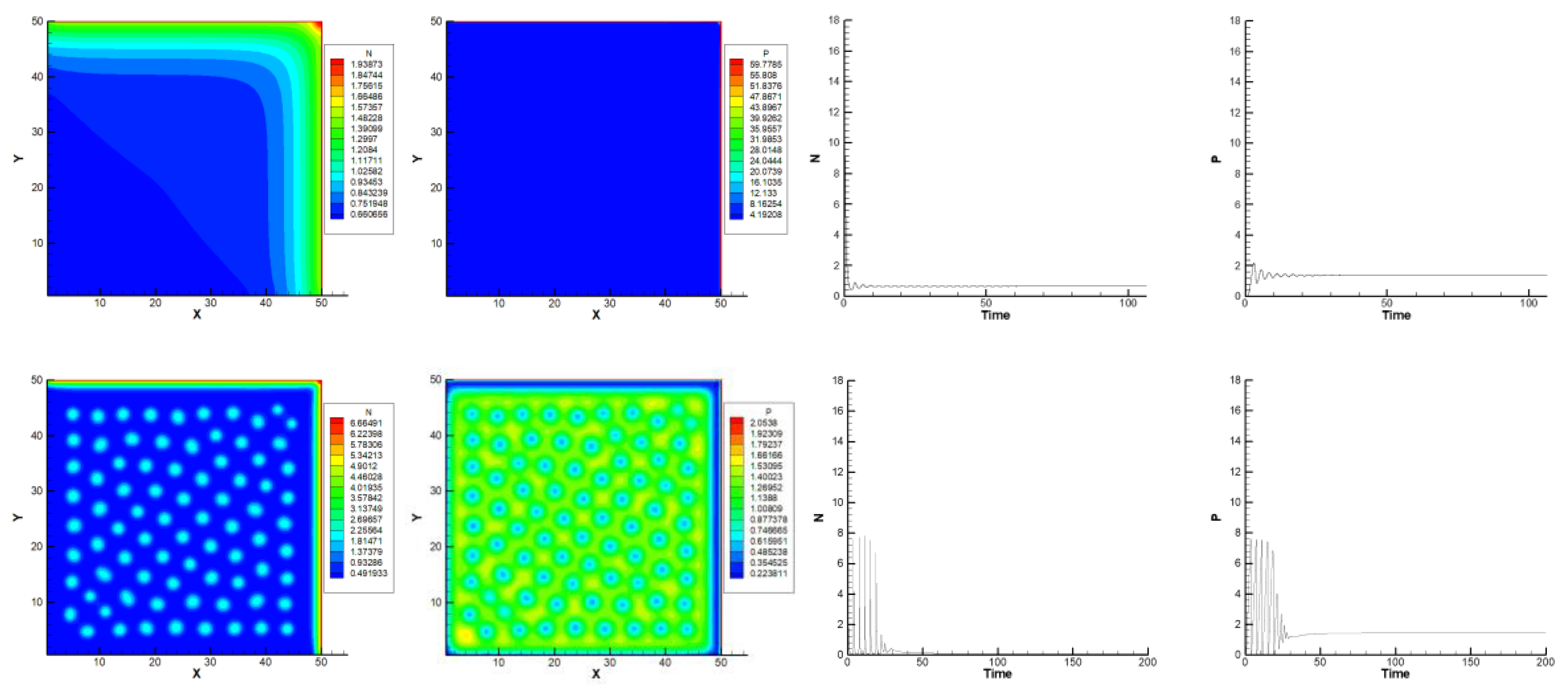
Figure 5 shows that there are reduced to zero patterns when d = 0.01 (above) and d = 10 (below). Outside of this range, there will be no pattern, while, in Figure 6, when d = 0.1, 1, and 3, the onset of a typical stripped Turing-style pattern can be seen. The ratio d for the Turing bifurcations could happen from 0.01 to 10, where we can find some thin stripes, and the number of stripes decreases when d increases.

Figure 5 shows the random distribution of plankton, forming a labyrinth pattern, and then the dying out of patches to form thin stripes depending on the ratio d variation in Figure 6. The number of stripes reduces in the function of time at the marginal d values of the range (0.01–10) (Figure 6).

3.2. Effects of γ

The parameter ‘γ’ represents the relative strength of the reactive functions. Mathematically, it is directly proportional to the linear dimension of the spatial domain or the surface area, implying that an increase in γ proportionally increases the activity rate. This step would be the limiting step in the reaction sequence. Biologically, it could be understood that γ represents the ability of cyanobacteria to capture and consume nutrients in space, herein the water surface area.

The analysis also highlighted the inverse relationship between γ and d as the diffusion ratio increased, and maintaining a stable pattern required a corresponding adjustment in γ values. This relationship underscores the balance needed between nutrient availability and cyanobacterial mobility to sustain spatial structures in HABs.

It can also be said that γ is inversely proportional to d, where d = D_inhibitor/De_activator.

Figure 7 showed the patterns appearing in different values of γ = 10, 5, and 0.1 (other parameters were a = 0.01; b = 0.05; d = 3 (0.9/0.3); Vp = 3). The patterns disappear when γ is less than 1.

3.3. Simulated Patterns and Real Field Observations

Our simulation results showed two general categories of obtained patterns: cloud-like patterns and strips. Some real patterns were observed and could be compared with the simulated Turing’s generic shapes.

A key aspect of this study involved comparing simulated HAB patterns with aerial images captured by drones over Torment Lake in September 2023. The simulated results displayed two primary types of patterns: cloud-like structures and strip formations. These patterns were similar to those observed in real HABs, where cyanobacterial blooms formed patchy, cloud-like appearances during their early stages and evolved into more organized, stripe-like patterns as they developed. For example, the bloom images in Figure 8 resemble the simulated cloudy-striped patterns, while Figure 9 highlights the onset of striped formations seen both in simulations and real field observations.

This qualitative agreement between simulations and drone imagery suggested that the model can accurately capture key aspects of HAB dynamics. While the scale and exact arrangement of the patterns vary due to environmental complexities, the model’s ability to replicate similar generic shapes is promising for future predictive applications.

Figure 10 and Figure 11 showed the bloom onset and then a developed blooming period at a large area of Dolichospermum flos-aquae and Anathece Bachmannii species taken in the waters of Torment Lake (Nova Scotia, Canada) in 2023. Simulated banded patterns are likely observed patterns.

It can be noticed that the pattern formation depends on the variation in the ratio d, ${\overrightarrow{ v}}_P$, and γ.

Figure 12 and Figure 13 show various aspects of Turing’s instability involved in HAB patterning at different periods and with various parameters g and ${\overrightarrow{ v}}_P$. Although our simulated results can present some significant analogies to the real patterns, it is noted that we can only compare the generic shapes or types of patterning due to the anonymity of the real pattern scales. Further research and study are envisaged to explore more qualitative and quantitative comparisons on the spatial dimension of HAB real patterns with the simulated results.

While the model successfully simulates the key aspects of HAB pattern formation, certain limitations remain. The current approach did not include hydrodynamic effects from water flow, which may influence the spread and organization of cyanobacterial blooms in real ecosystems. Additionally, while the comparisons with drone images provide valuable insights, further validation with quantitative field data, such as cell counts and nutrient concentrations, is necessary. Incorporating these data will enhance the model’s accuracy and predictive power, making it a more effective tool for forecasting HABs and managing water quality in affected regions.

4. Conclusions

We proposed a modeling approach based on Turing’s instability to address harmful algal bloom (HAB) patterns in lentic water, showing promising similarities between simulated and real-world patterns. Future studies will couple the model with the Navier–Stokes equations to include hydrodynamic effects, as the current RK4 method may not handle the complexity of these high-order systems. Additionally, the model aimed to enhance the understanding of algal blooms to improve monitoring and management efforts, focusing on identifying biophysical thresholds and quantifying toxin levels. Given the complexity and nonlinearity of bloom dynamics, further research is needed to refine predictive capabilities and identify critical environmental conditions.

In future work, we plan to integrate drone imagery with AI and machine learning to analyze large datasets, allowing for real-time detection and improved prediction of HAB dynamics. This approach, combined with environmental variables such as temperature, nutrient levels, and light intensity, will enhance forecasting and decision-making for water resource management. While deterministic models offer precision for stable conditions, stochastic models can better address variability and uncertainty in bloom behavior. However, all models must be rigorously validated through field data and lab analyses to ensure their accuracy and broader applicability.