A Rule-Based Method to Locate the Bounds of Neural Networks

Abstract

An advanced method of training artificial neural networks is presented here which aims to identify the optimal interval for the initialization and training of artificial neural networks. The location of the optimal interval is performed using rules evolving from a genetic algorithm. The method has two phases: in the first phase, an attempt is made to locate the optimal interval, and in the second phase, the artificial neural network is initialized and trained in this interval using a method of global optimization, such as a genetic algorithm. The method has been tested on a range of categorization and function learning data and the experimental results are extremely encouraging.

1. Introduction

Artificial neural networks (ANNs) are programming tools [1,2] based on a series of parameters that are commonly called weights or processing units. They have been used in a variety of problems from different scientific areas, such as physics [3,4,5], solving differential equations [6,7], agriculture [8,9], chemistry [10,11,12], economics [13,14,15], medicine [16,17], etc. A common way to express a neural network is a function $N(\overrightarrow{x},\overrightarrow{w})$, with $\overrightarrow{x}$ the input vector (commonly called the pattern) and $\overrightarrow{w}$ the weight vector. A method that trains a neural network should be used to estimate the vector $\overrightarrow{w}$ for a certain problem. The training procedure can also be formulated as an optimization problem, where the target is to minimize the so-called error function:

$$E\left(N\left(\overrightarrow{x},\overrightarrow{w}\right)\right)=\sum _{i=1}^M{\left(N\left({\overrightarrow{x}}_i,\overrightarrow{w}\right)-y_i\right)}^2$$

(1)

In Equation (1), the set $\left(\overrightarrow{x_i},y_i\right),i=1,\dots ,M$, is the dataset used to train the neural network, with $y_i$ being the actual output for the point $\overrightarrow{x_i}$. The neural network $N(\overrightarrow{x},\overrightarrow{w})$ can be modeled as a summation of processing units, as proposed in [18]:

$$N\left(\overrightarrow{x},\overrightarrow{w}\right)=\sum _{i=1}^H{w}_{(d+2)i-(d+1)}\sigma \left(\sum _{j=1}^d{x}_j{w}_{(d+2)i-(d+1)+j}+w_{(d+2)i}\right)$$

(2)

with H the number of processing units in the neural network and d the dimension of vector $\overrightarrow{x}$. The function $\sigma \left(x\right)$ is the sigmoid function defined as:

$$\sigma \left(x\right)=\frac{1}{1+exp(-x)}$$

(3)

From Equation (2), one can obtain that the dimension of the weight vector w is computed as: $n=(d+2)H$. The function of Equation (1) has been minimized with a variety of optimization methods during the past years such as: the back propagation method [19,20], the RPROP method [21,22,23], quasi-Newton methods [24,25], simulated annealing [26,27], genetic algorithms [28,29], particle swarm optimization [30,31] etc. In addition, various researchers have worked on the initialization of the weights of neural networks, such as initialization using decision trees [32], an initialization method based on Cauchy’s inequality [33], a method based on discriminant learning [34], etc. Another topic that has attracted the interest of many researchers is weight decaying, which is a regularization method that adapts the weights of the network aiming to avoid the overfitting problem. Several papers have appeared in this area with methods such as those with positive correlation [35], the SarProp algorithm [36], the incorporation of pruning techniques [37], etc. In addition, more advanced and more recent techniques from the area of computational intelligence have been proposed for neural network training such as the differential evolution method [38,39], the construction of neural networks with ant colony optimization [40], the construction of neural networks using grammatical evolution to solve differential equations [41], etc. Furthermore, due to development of GPU units, a lot of works have been published that take advantage of these processing units [42,43].

The present work proposes an innovative interval generation technique for the initialization and training of artificial neural network parameters. This new method has its roots in interval methods [44,45,46]. In the current work, using arithmetic intervals, a set of rules for dividing the initial interval for the parameters of an artificial neural network is constructed. The construction is carried out using a hybrid genetic algorithm, in which chromosomes are the set of division rules. After the termination of the genetic algorithm, the artificial neural network is initialized in the interval resulting from the application of the optimal partitioning rules and then trained using a genetic algorithm.

The method used has two objectives: the first objective is to detect a small interval of initialization for the parameters of the artificial neural network and the second objective is to accelerate the training of the network. In the first target, using information from the training data, the algorithm will make an attempt to identify the interval that will ultimately give better results. In the second objective, once a small-value interval has been detected, a global optimization method can be used more efficiently to detect the lowest value of the network error.

The proposed method is expected to achieve significant results since in principle it has all the advantages of genetic algorithms, such as tolerance for errors, possibilities for parallel implementation, the efficient exploration of the research space, etc. In addition, the first phase of the method will reduce the volume of the possible values for the weights so that in the second phase the search for the global minimum of the network error function will become more efficient and faster.

The proposed methodology can even be applied to different types of artificial neural networks such as recurrent neural networks [47,48]. A simple recurrent neural network can be expressed as single neural cell with a single input, a single output and a state (also known as the memory of the cell). Given the input of the cell $x\left(t\right)$ at step t and the previous state of the cell $h(t-1)$ at step $t-1$, the updated state of the cell $h\left(t\right)$ is estimated as shown in the equation:

$$\mathbf{h}\left(t\right)=f\left({\mathbf{W}}_{hh}\ast \mathbf{h}(t-1)+{\mathbf{W}}_{xh}\ast \mathbf{x}\left(t\right)+{\mathbf{b}}_h\right)$$

(4)

$$\mathit{y}\left(t\right)=\sigma \left({\mathit{W}}_{hy}\ast h\left(t\right)+{\mathit{b}}_y\right)$$

(5)

where the $f\left(x\right)$ function is usually the softmax function. The proposed method can be used here to estimate a promising bounding box for the vector parameters $\mathbf{W}$ and $\mathbf{b}$ of the network before any other training method is applied.

The rest of this article is as follows: in Section 2 the proposed method is discussed in detail, in Section 3 the experimental datasets as well as the results from the application of the proposed method are provided and finally in Section 4 some conclusions and guidelines for future enhancements are presented.

2. Method Description

The proposed method consists of two major steps: in the first step, the construction of partition rules for the initial value interval for the parameters of the artificial neural network is made, and in the second step, the artificial neural network is initialized in the optimal space resulting from the first step and training takes place. The training is performed through a second genetic algorithm. In the first genetic algorithm, the chromosomes are sets of partition rules for the initial value interval of the artificial neural network, and in the second genetic algorithm, the chromosomes are the parameters of the artificial neural network. It is obvious that this is a time-consuming process and modern parallel techniques such as the OpenMP [49] library must be used to accelerate it. The first genetic algorithm is analyzed in Section 2.1 and the second in Section 2.5.

2.1. Locating the Best Rules

Firstly, we introduce the rule set $I_n$ where:

$$I_n=\left\{\left(l_1,r_1\right),\left(l_2,r_2\right),\dots ,\left(l_n,r_n\right)\right\}$$

(6)

where $l_i\in \left\{0,1\right\},r_i\in \left\{0,1\right\}$ and $i=1,\dots ,n$. The set $I_n$ defines the set of partition rules for a function defined as

$$f:S\to R,S\subset R^n$$

(7)

with S:

$$S=\left[a_1,b_1\right]\otimes \left[a_2,b_2\right]\otimes \dots \left[a_n,b_n\right]$$

(8)

If $l_i=1$ then $a_i=\frac{a_i}{2}$ and if $r_i=1$ then $b_i=\frac{b_i}{2}$. For example, consider the Rastrigin function:

$$f\left(x\right)=x_1^2+x_2^2-cos\left(18x_1\right)-cos\left(18x_2\right),x\in {[-1,1]}^2$$

(9)

Also consider the set $I_2=\left\{\left(1,0\right),\left(0,1\right)\right\}$. The produced bounding box for the Rastrigin function is now $S^{\prime }=\left[-0.5,1\right]\times \left[-1,0.5\right]$.

Subsequently, we introduce the extended set $C_{Kn}$ as a set of production rules defined as:

$$R_{Kn}=\left\{I_n^{\left(1\right)},I_n^{\left(2\right)},\dots ,I_n^{\left(K\right)}\right\},$$

(10)

where $I_n^{\left(i\right)},i=1,\dots ,K$, are the rule sets of Equation (6). For example, let $K=2$ for the Rastrigin function and $R_{22}=\left\{\left\{\left(0,1\right),\left(1,0\right)\right\},\left\{\left(1,0\right),\left(1,1\right)\right\}\right\}$. The final bounding box is considered after applying the sets $\left\{\left(0,1\right),\left(1,0\right)\right\}$ and $\left\{\left(1,0\right),\left(1,1\right)\right\}$ in the original box S. The computation steps are:

• Apply$\left\{\left(0,1\right),\left(1,0\right)\right\}$ to S, yielding $S^{\prime }=\left[-0.5,1\right]\times \left[-1,0.5\right]$.
• Apply$\left\{\left(1,0\right),\left(1,1\right)\right\}$ to $S^{\prime }$, yielding $S^{″}=\left[-0.25,1\right]\times \left[-0.5,0.25\right]$.

We consider chromosomes in the form of Equation (10) for the first phase of the proposed method. The value n is the total number of parameters for the neural network. The fitness of every chromosome g is an interval $f_g=\left[f_{g,\min },f_{g,\max }\right]$. Hence, in order to compare two different intervals $a=\left[a_1,a_2\right]$ and $b=\left[b_1,b_2\right]$, we incorporate the following function:

$$\begin{array}{ccc}\hfill L^{*}(a,b)& =& \left\{\begin{array}{cc}\mathrm{TRUE},\hfill & a_1<b_1,\mathrm{OR}\left(a_1=b_1\mathrm{AND}{a}_2<b_2\right)\hfill \\ \mathrm{FALSE},\hfill & \mathrm{OTHERWISE}\hfill \end{array}\right.\hfill \end{array}$$

(11)

Hence, the steps of the genetic algorithm of the first phase are the following:

2.1.1. Initialization Step

• SetK as the number of rules.
• Set$S={\left[-D,D\right]}^n$ as the initial bounding box for the parameters of the neural network. D is considered as a positive number with $D>1$.
• Set$N_C$ as the total number of chromosomes.
• Set$N_S$ as the number of samples in the fitness evaluation.
• Set$P_s$ as the selection rate, where $P_s\le 1$.
• Set$P_m$ as the mutation rate, where $P_m\le 1$.
• Set$t=0$ as the current generation number.
• Set$N_t$ as the maximum number of generations allowed.
• Initialize randomly the chromosomes $C_i,i=1,\dots ,N_C$, as sets of Equation (10).

2.1.2. Termination Check Step

• Set$t=t+1$.
• If$t\ge N_t$, terminate.

2.1.3. Genetic Operations Step

• For every chromosome $C_i,i=1,\dots ,N_C$, calculate the corresponding fitness value $f_i$ using the algorithm in Section 2.2.
• Apply the selection operator. Initially, the chromosomes are sorted according to their fitness values. The sorting utilizes the function $L^{*}(a,b)$ of Equation (11) to compare fitness values. The best $\left(1-P_s\right)\times N_c$ are copied to the next generation while the rest of them are substituted by offspring created through the crossover procedure. The mating parents for the crossover procedure are selected using the well-known technique of tournament selection.
• Apply the crossover operator: For every pair of selected parents $(z,w),$ two children $(cz,cw)$ are produced using the uniform crossover procedure described in Section 2.3.
• Apply the mutation operator using the algorithm in Section 2.4.
• Goto Termination Check Step.

2.2. Fitness Evaluation for the Rule Genetic Algorithm

The fitness value for each chromosome g is considered as an interval $f=\left[f_{\min },f_{\max }\right]$, where $f_{\min }$ is an estimation of the lower value obtained using the rules of the chromosome g and $f_{\max }$ is an estimation of the maximum value. In order to calculate the fitness of every set of rules C, the following steps are performed:

• Set$f_{\min }=\infty$.
• Set$f_{\max }=-\infty$.
• Apply the rule set g to the original bounding box S. The outcome of this application is the new bounding box $S_g$.
• For$i=1,\dots ,N_S$do

  (a)

  Produce a random sample $w\in S_g$.

  (b)

  Calculate the training error $E_g=E(N(\overrightarrow{x},\overrightarrow{w}))$ using Equation (1).

  (c)

  If$E_g\le f_{\min }$ then $f_{\min }=E_g$.

  (d)

  If$E_g\ge f_{\max }$ then $f_{\max }=E_g$.

• EndFor
• Return the interval $f=\left[f_{\min },f_{\max }\right]$ as the fitness of chromosome $g.$

2.3. Crossover for the Rule Genetic Algorithm

The crossover for the genetic algorithm of the first phase is performed using uniform crossover. For every couple $(z,w)$ of selected parents, two children $(cz,cw)$ are produced through the following procedure:

• For$i=1\dots K$do

  (a)

  Let$z^{\left(i\right)}=\left\{l_z^{\left(i\right)},r_z^{\left(i\right)}\right\}$ be the i-th item of the chromosome z.

  (b)

  Let$w^{\left(i\right)}=\left\{l_w^{\left(i\right)},r_w^{\left(i\right)}\right\}$ be the i-th item of the chromosome w.

  (c)

  Produce a random number $r\le 1$.

  (d)

  If$r\le 0.5$then

  • Set${cz}^{\left(i\right)}=\left\{l_z^{\left(i\right)},r_w^{\left(i\right)}\right\}$.
  • Set${cw}^{\left(i\right)}=\left\{l_w^{\left(i\right)},r_z^{\left(i\right)}\right\}$.

  (e)

  Else

  • Set${cz}^{\left(i\right)}=\left\{l_w^{\left(i\right)},r_z^{\left(i\right)}\right\}$.
  • Set${cw}^{\left(i\right)}=\left\{l_z^{\left(i\right)},r_w^{\left(i\right)}\right\}$.

  (f)

  Endif

• EndFor

2.4. Mutation for the Rule Genetic Algorithm

The steps for the mutation procedure for the genetic algorithm of the first phase are the following:

• For$i=1,\dots ,N_C$do

  (a)

  Let$C_i=\left\{C_i^{\left(1\right)},C_i^{\left(2\right)},\dots ,C_i^{\left(K\right)}\right\}$ be the i-th chromosome of the population.

  (b)

  For$j=1,\dots ,K$do

  • Let$C_i^{\left(j\right)}=\left\{l_i^{\left(j\right)},r_i^{\left(j\right)}\right\}$.
  • Take$r\le$1 a random number.
  • If$r\le P_m$then alter randomly with probability 50% the $l_i^{\left(j\right)}$ or the $r_i^{\left(j\right)}$ part of $C_i^{\left(j\right)}$.

  (c)

  EndFor

• EndFor

2.5. Second Phase

In the second phase, the best chromosome $g_b$ defined as

$$g_b=\left\{\left\{l_{b,1},r_{b,1}\right\},\left\{l_{b,2},r_{b,2}\right\},\dots ,\left\{l_{b,K},r_{b,K}\right\}\right\}$$

(12)

is used to transform the original bounding box $S={[-F,F]}^{\left(n\right)}$ into a new box $S_b$. The new hyperbox is defined as

$$S_b=\left[a_{g,1},b_{g,1}\right]\times \left[a_{g,2},b_{g,2}\right]\times \dots \times \left[a_{g,n},b_{g,n}\right]$$

(13)

This hyperbox will be used to bound the parameters of the neural network. The parameters of the network are trained using a genetic algorithm with the following steps:

2.5.1. Initialization Step

• Set$N_C$ as the total number of chromosomes.
• Set$P_s$ as the selection rate, where $P_s\le 1$.
• Set$P_m$ as the mutation rate, where $P_m\le 1$.
• Set$t=0$ as the current generation number.
• Set$N_t$ as the maximum number of generations allowed.
• Initialize randomly the chromosomes $C_i,i=1,\dots ,N_C$, inside the bounding box $S_b$.

2.5.2. Termination Check Step

• Set$t=t+1$.
• If$t\ge N_t$goto Local Search Step.

2.5.3. Genetic Operations Step

• Calculate the fitness value of every chromosome.

  (a)

  For$i=1\dots N_C$Do

  • Set$f_i=E(N(\overrightarrow{x},C_i))$ using Equation (1).

  (b)

  EndFor

• Apply the crossover operator. In this phase, the best $\left(1-P_s\right)\times N_c$ chromosomes are transferred intact to the next generation. The rest of the chromosomes are substituted by offspring created through crossover. The selection of two parents $x=\left(x_1,x_2,\dots ,x_n\right)$ and $y=\left(y_1,y_2,\dots ,y_n\right)$ for crossover is performed using tournament selection. Having selected the parents, the offspring $\tilde{x}$ and $\tilde{y}$ are formed using the following:

  $$\begin{array}{ccc}\hfill \widetilde{x_i}& =& r_i{x}_i+\left(1-r_i\right)y_i\hfill \\ \hfill \widetilde{y_i}& =& r_i{y}_i+\left(1-r_i\right)x_i\hfill \end{array}$$

  (14)

  where $r_i$ are random numbers in $[-0.5,1.5]$ [43].
• Apply the mutation operator. The mutation scheme is the same as in the work of Kaelo and Ali [50]:

  (a)

  For$i=1\dots N_C$do

  • For$j=1\dots n$do
    • Let$r\in [0,1]$ be a random number.
    • If$r\le P_m$ alter the element $C_{ij}$ using the following:

      $$C_{ij}=\left\{\begin{array}{cc}{C}_{ij}+\Delta \left(t,b_{g,i}-C_{ij}\right)& t=0\\ C_{ij}-\Delta \left(t,C_{ij}-a_{g,i}\right)& t=1\end{array}\right.$$

      (15)

      where t is a random number that takes either the value 0 or 1 and $\Delta (t,y)$ is calculated as:

      $$\Delta (t,y)=y\left(1-r^{\left(1-\frac{t}{N_t}\right)z}\right)$$

      (16)

      where $r\in [0,1]$ is a random number and z is a user-defined parameter.
  • EndFor

  (b)

  EndFor

• Goto Termination check step.

2.5.4. Local Search Step

• Set$C^{*}$ as the best chromosome of the population.
• Apply a local search procedure $C^{*}=\mathcal{L}\left(C^{*}\right)$. The local search procedure used here is a BFGS method of Powell [51].

3. Experiments

The proposed method was evaluated on a series of classification and regression problems from the relevant literature. The classification problems used for the experiments were found in most cases in two internet databases:

• UCI dataset repository, https://archive.ics.uci.edu/ml/index.php (accessed on 23 May 2022.)
• Keel repository, https://sci2s.ugr.es/keel/datasets.php (accessed on 23 May 2022) [52].

The regression datasets were in most cases available from the Statlib URL http://lib.stat.cmu.edu/datasets/ (accessed on 23 May 2022). The proposed method was compared against a neural network trained by a genetic algorithm and the results are reported.

3.1. Experimental Datasets

The following classification datasets were used:

• Appendicitis, a medical dataset, proposed in [53].
• Australian dataset [54], which is related to credit card applications.
• Balance dataset [55], which is used to predict psychological states.
• Cleveland dataset, a dataset used to detect heart disease used in various papers [56,57].
• Bands dataset, a printing problem used to identify cylinder bands.
• Dermatology dataset [58], which is used for the differential diagnosis of erythemato-squamous diseases.
• Hayes Roth dataset. This dataset [59] contains 5 numeric-valued attributes and 132 patterns.
• Heart dataset [60], used to detect heart disease.
• HouseVotes dataset [61], which is about votes for U.S. House of Representatives Congressmen.
• Ionosphere dataset. The ionosphere dataset contains data from the Johns Hopkins Ionosphere database and it has been studied in several papers [62,63].
• Liverdisorder dataset [64], used for detecting liver disorders in people using blood analysis.
• Mammographic dataset [65]. This dataset be used to identify the severity (benign or malignant) of a mammographic mass lesion from BI-RADS attributes and the patient’s age. It contains 830 patterns of 5 features each.
• PageBlocks dataset [66], used to detect the page layout of a document.
• Parkinsons dataset. This dataset is composed of a range of biomedical voice measurements from 31 people, 23 with Parkinson’s disease (PD) [67].
• Pima dataset [68], used to detect the presence of diabetes.
• Popfailures dataset [69], which is related to climate model simulation crashes of simulation crashes.
• Regions2 dataset. It is created from liver biopsy images of patients with hepatitis C [70]. From each region in the acquired images, 18 shape-based and color-based features were extracted, while it was also annotated by medical experts. The resulting dataset includes 600 samples belonging to 6 classes.
• Saheart dataset [71], used to detect heart disease.
• Segment dataset [72]. This database contains patterns from a database of 7 outdoor images (classes).
• Wdbc dataset [73], which contains data for breast tumors.
• Wine dataset, used to detect through chemical analysis the origin of wines and has been used in various research papers [74,75].
• Eeg datasets. As a real-world example, consider an EEG dataset described in [9] is used here. The dataset consists of five sets (denoted as Z, O, N, F and S) each containing 100 single-channel EEG segments each having 23.6 sec duration. With different combinations of these sets, the produced datasets are Z_F_S, ZO_NF_S and ZONF_S.
• ZOO dataset [76], where the task is to classify animals in seven predefined classes.

In addition, the following regression datasets were used:

• ABALONE dataset [77]. This dataset can be used to obtain a model to predict the age of abalone from physical measurements.
• AIRFOIL dataset, which is used by NASA for a series of aerodynamic and acoustic tests [78].
• BASEBALL dataset, a dataset to predict the salary of baseball players.
• BK dataset. This dataset comes from smoothing methods in statistics [79] and is used to estimate the points scored per minute in a basketball game.
• BL dataset: This dataset can be downloaded from StatLib. It contains data from an experiment on the effects of machine adjustments on the time to count bolts.
• CONCRETE dataset. This dataset is taken from civil engineering [80].
• DEE dataset, used to predict the daily average price of electricity energy in Spain.
• DIABETES dataset, a medical dataset.
• HOUSING dataset. This dataset was taken from the StatLib library which is maintained at Carnegie Mellon University and it is described in [81].
• FA dataset, which contains percentage of body fat and ten body circumference measurements. The goal is to fit body fat to the other measurements.
• MB dataset. This dataset is available from smoothing methods in statistics [79] and it includes 61 patterns.
• MORTGAGE dataset, which contains the economic data information of the U.S.
• PY dataset (pyrimidines problem). The source of this dataset is the URL https://www.dcc.fc.up.pt/~ltorgo/Regression/DataSets.html (accessed on 23 May 2022) and it is a problem of 27 attributes and 74 patterns. The task consists of learning quantitative structure activity relationships (QSARs) and is provided by [82].
• QUAKE dataset. The objective here is to approximate the strength of an earthquake.
• TREASURY dataset, which contains economic data information of the U.S. from 1 April 1980 to 2 April 2000 on a weekly basis.
• WANKARA dataset, which contains weather information.

3.2. Experimental Results

The method was compared against three other methods:

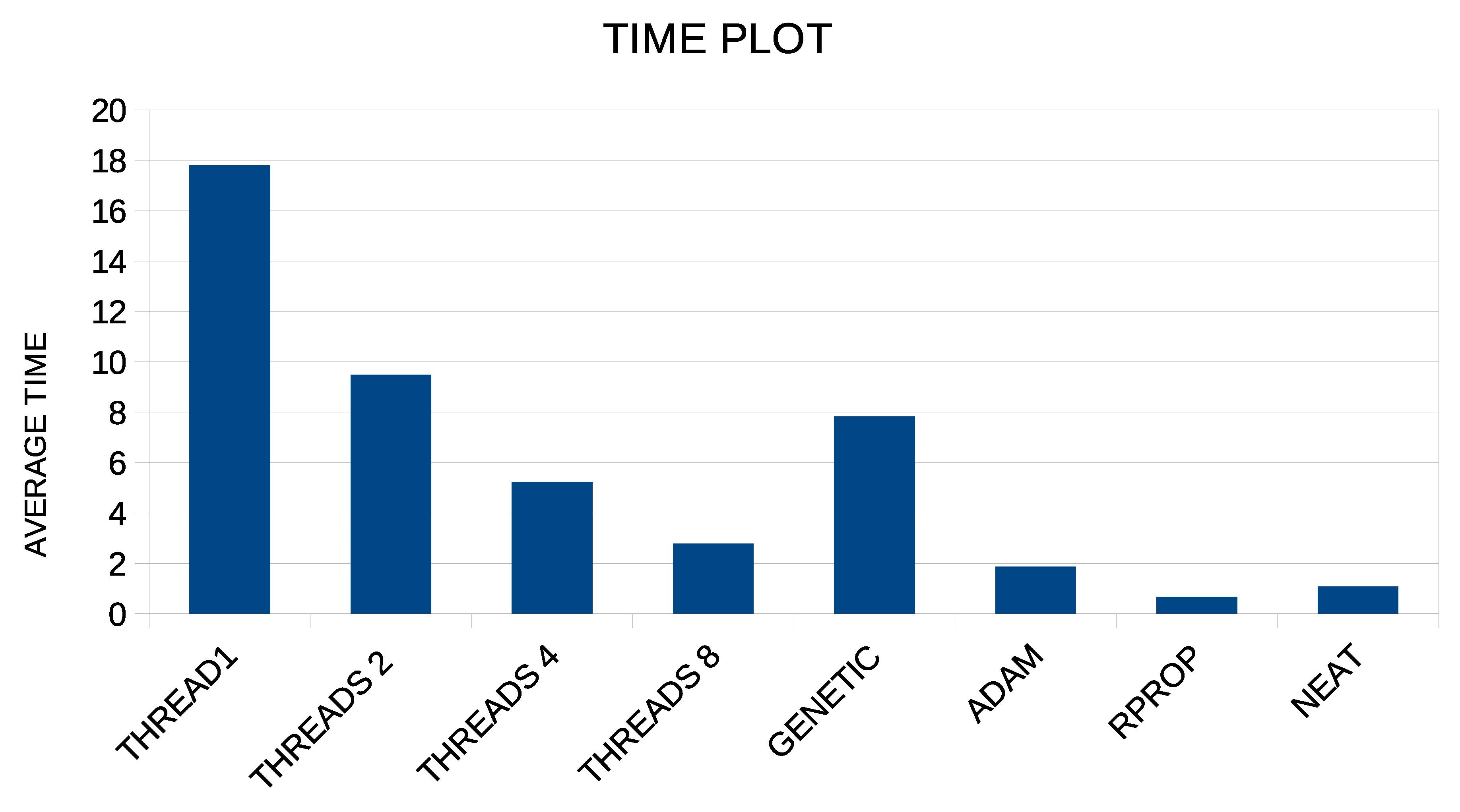
• A genetic algorithm with the same parameters that are shown in

  Table 1. Experimental parameters.

  PARAMETER	VALUE
  K	20
  H	10
  $N_C$	200
  $N_S$	50
  $N_t$	200
  $P_s$	0.10
  $P_m$	0.01

  . In addition, after the termination of the genetic algorithm, the local search procedure of BFGS was applied to the best chromosome of the population, in order to enhance the quality of the solution. The column GENETIC in the experimental tables denotes the results from the application of this method.
• The Adam stochastic optimization method [83] as implemented in OptimLib, freely available from https://github.com/kthohr/optim (accessed on 23 May 2022). The results for this method are listed in the column ADAM in the relevant tables.
• The RPROP method [21] as implemented in the FCNN software package [84]. The results for this method are listed in the column RPROP in the relevant tables.
• The NEAT method (neuroevolution of augmenting topologies) [85] as implemented in the EvolutionNet package which is freely available from https://github.com/BiagioFesta/EvolutionNet (accessed on 23 May 2022). The maximum number of generations was the same as in the case of the genetic algorithm.

All the experiments were conducted 30 times with different seeds for the random number generator each time and averages were taken. To perform the experiments, the software IntervalGenetic is freely available from https://github.com/itsoulos/IntervalGenetic (accessed on 23 May 2022) was utilized. The experimental results for the classification datasets are shown in

Table 2. Experiments for classification datasets.

DATASET	GENETIC	ADAM	RPROP	NEAT	$\mathit{D}=50$	$\mathit{D}=100$	$\mathit{D}=200$
Appendicitis	18.10%	16.50%	16.30%	17.20%	15.00%	14.00%	16.07%
Australian	32.21%	35.65%	36.12%	31.98%	24.85%	30.20%	28.52%
Balance	8.97%	7.87%	8.81%	23.14%	7.42%	7.42%	7.67%
Bands	35.75%	36.25%	36.32%	34.30%	32.00%	32.25%	33.06%
Cleveland	51.60%	67.55%	61.41%	53.44%	41.64%	44.66%	44.39%
Dermatology	30.58%	26.14%	15.12%	32.43%	15.49%	11.00%	10.80%
Hayes Roth	56.18%	59.70%	37.46%	50.15%	28.72%	28.84%	32.05%
Heart	28.34%	38.53%	30.51%	39.27%	15.58%	17.07%	16.22%
HouseVotes	6.62%	7.48%	6.04%	10.89%	3.92%	3.78%	3.26%
Ionosphere	15.14%	16.64%	13.65%	19.67%	12.25%	9.71%	7.12%
Liverdisorder	31.11%	41.53%	40.26%	30.67%	30.90%	29.54%	30.70%
Lymography	23.26%	29.26%	24.67%	33.70%	18.98%	17.52%	17.67%
Mammographic	19.88%	46.25%	18.46%	22.85%	17.01%	17.60%	15.97%
PageBlocks	8.06%	7.93%	7.82%	10.22%	7.73%	7.01%	6.71%
Parkinsons	18.05%	24.06%	22.28%	18.56%	14.81%	13.86%	12.53%
Pima	32.19%	34.85%	34.27%	34.51%	23.51%	25.31%	27.49%
Popfailures	5.94%	5.18%	4.81%	7.05%	6.13%	5.93%	5.30%
Regions2	29.39%	29.85%	27.53%	33.23%	24.01%	23.14%	23.62%
Saheart	34.86%	34.04%	34.90%	34.51%	28.94%	29.04%	29.93%
Segment	57.72%	49.75%	52.14%	66.72%	47.38%	49.49%	40.61%
Wdbc	8.56%	35.35%	21.57%	12.88%	6.23%	5.28%	5.49%
Wine	19.20%	29.40%	30.73%	25.43%	5.51%	6.55%	6.22%
Z_F_S	10.73%	47.81%	29.28%	38.41%	4.70%	5.61%	6.01%
ZO_NF_S	8.41%	47.43%	6.43%	43.75%	5.39%	4.67%	5.81%
ZONF_S	2.60%	11.99%	27.27%	5.44%	1.85%	2.07%	2.24%
ZOO	16.67%	14.13%	15.47%	20.27%	14.83%	11.40%	8.50%
AVERAGE	23.47%	30.81%	25.37%	28.87%	17.49%	17.42%	17.08%

and the results for the regression datasets are outlined in

Table 3. Experiments for regression datasets.

DATASET	GENETIC	ADAM	RPROP	NEAT	$\mathit{D}=50$	$\mathit{D}=100$	$\mathit{D}=200$
ABALONE	7.17	4.30	4.55	9.88	4.22	4.18	3.89
AIRFOIL	0.003	0.005	0.002	0.067	0.003	0.003	0.003
BASEBALL	103.60	77.90	92.05	100.39	49.47	51.07	53.57
BK	0.027	0.03	1.599	0.15	0.017	0.017	0.019
BL	5.74	0.28	4.38	0.05	0.0019	0.0016	0.0016
CONCRETE	0.0099	0.078	0.0086	0.081	0.0053	0.0044	0.0042
DEE	1.013	0.63	0.608	1.512	0.187	0.205	0.203
DIABETES	19.86	3.03	1.11	4.25	0.31	0.31	0.29
HOUSING	43.26	80.20	74.38	56.49	19.28	18.50	17.75
FA	1.95	0.11	0.14	0.19	0.011	0.012	0.012
MB	3.39	0.06	0.055	0.061	0.048	0.047	0.047
MORTGAGE	2.41	9.24	9.19	14.11	0.57	0.70	0.53
PY	105.41	0.09	0.039	0.075	0.016	0.014	0.014
QUAKE	0.040	0.06	0.041	0.298	0.036	0.036	0.036
TREASURY	2.929	11.16	10.88	15.52	0.473	0.677	0.622
WANKARA	0.012	0.02	0.0003	0.005	0.0003	0.0002	0.0002
AVERAGE	18.55	11.70	12.44	12.70	4.67	4.74	4.81

. For the classification problems, the average classification error on the test set is shown, and for regression datasets, the average mean squared error on the test set is displayed. In all cases, 10-fold cross validation was used and the number of hidden nodes (parameter H) was set to 10. The column DATASET stands for the name of the dataset incorporated, the column $D=50$ represents the application of the proposed method with $D=50$ as the initial value for the interval of weights, the column $D=100$ stands for the results of the proposed method with $D=100$ and finally the column $D=200$ represents the results of the proposed method with $D=200$. In both tables, an additional row was added at the end showing the average classification or regression error for all datasets and it is denoted by the name AVERAGE. All the experiments were conducted on an AMD Ryzen 5950X equipped with 128 GB of RAM. The operating system used was OpenSUSE Linux and all the programs were compiled using the GNU C++ compiler.

As can be seen from the experimental results, the proposed method is significantly superior to the other methods, especially in the case of regression data. The RPROP training method seems to overcome ADAM in most cases of classification datasets and the simple genetic method is better than ADAM and RPROP for classification datasets but not for regression datasets. In addition, the change in the parameter D does not seem to have a significant effect on the performance of the algorithm and the proposed algorithm achieves high performance even for small values of this parameter.

In addition, the average execution times for all the problems of this publication were compared between the proposed method and the methods ADAM, RPROP, GENETIC and NEAT mentioned above. The average execution times are presented graphically in Figure 1. In order to speed up the proposed method, the genetic algorithm used was parallelized using the open source library OpenMP [49]. The column THREAD1 stands for the average time execution of the proposed method with one thread, the column THREADS 2 represents the average execution time of the proposed method using two threads in the OpenMP implementation, the column THREADS 4 denotes the average execution time of the proposed method for four threads and finally the column THREADS 8 denotes the average execution time for eight threads for the OpenMP implementation. The proposed method has slow execution times when performed on one thread, but as the number of threads used increases, the execution time decreases dramatically. This is very important, because it means that it could be used in large problems if the computer in use has enough execution threads. Obviously, all the methods of training artificial neural networks could be parallelized in one way or another. The parallelization of the proposed method was performed since it is by nature an extremely slow method, since it requires the use of two genetic algorithms in series. By using parallel techniques, this problem is alleviated; however, the computational cost remains high. However, this is the only substantial price for using this technique. In addition, a time comparison was made for the PageBlocks dataset between the proposed method and a parallel implementation of the Adam algorithm named DADAM for the number of threads ranging from 1 to 8. The time comparison is graphically illustrated in Figure 2.

To make the dynamics of the proposed method clearer, another series of experiments was performed. In these, the maximum number of generations (parameter $N_t$) received three values: 20, 40 and 100. For each value, all experiments for the classification and regression datasets were performed. The results for the classification datasets are listed in

Table 4. Experiments with $N_t$ for the classification datasets.

DATASET	${\mathit{N}}_{\mathit{t}}=20$	${\mathit{N}}_{\mathit{t}}=40$	${\mathit{N}}_{\mathit{t}}=100$
Appendicitis	15.23%	15.37%	15.77%
Australian	32.85%	33.15%	30.18%
Balance	11.92%	7.61%	8.71%
Bands	35.61%	33.86%	32.96%
Cleveland	43.91%	43.35%	41.29%
Dermatology	28.41%	21.28%	14.33%
Hayes Roth	50.33%	38.56%	36.80%
Heart	20.61%	21.16%	19.99%
HouseVotes	4.07%	4.31%	3.58%
Ionosphere	12.14%	11.19%	9.23%
Liverdisorder	31.47%	33.01%	31.24%
Lymography	22.24%	22.57%	20.74%
Mammographic	18.66%	17.37%	15.71%
PageBlocks	7.95%	7.68%	6.81%
Parkinsons	17.28%	17.44%	13.86%
Pima	33.19%	31.94%	30.71%
Popfailures	6.65%	5.81%	5.24%
Regions2	26.33%	26.03%	22.25%
Saheart	36.11%	32.96%	34.45%
Segment	66.37%	58.33%	49.85%
Wdbc	7.38%	6.95%	7.68%
Wine	13.49%	11.55%	8.39%
Z_F_S	7.77%	7.59%	8.38%
ZO_NF_S	8.21%	7.52%	7.28%
ZONF_S	2.26%	1.87%	1.99%
ZOO	14.70%	12.30%	13.50%
AVERAGE	22.12%	20.41%	18.88%

and the results for the regression datasets are shown in

Table 5. Experiments with different values of $N_t$ parameter for the regression datasets.

DATASET	${\mathit{N}}_{\mathit{t}}=20$	${\mathit{N}}_{\mathit{t}}=40$	${\mathit{N}}_{\mathit{t}}=100$
ABALONE	4.88	4.77	4.63
AIRFOIL	0.004	0.004	0.004
BASEBALL	69.83	65.37	69.72
BK	0.02	0.02	0.02
BL	0.006	0.005	0.007
CONCRETE	0.008	0.006	0.005
DEE	0.224	0.225	0.199
DIABETES	0.357	0.343	0.321
HOUSING	26.43	25.88	20.65
FA	0.019	0.019	0.017
MB	0.05	0.05	0.05
MORTGAGE	2.11	1.76	1.44
PY	0.02	0.018	0.022
QUAKE	0.042	0.037	0.037
TREASURY	2.37	2.12	1.48
WANKARA	0.0004	0.0003	0.0003
AVERAGE	6.65	6.29	6.16

. As expected, the proposed method improves its performance as the maximum number of generations increases, but even for a small number of generations it has a satisfactory performance.

In addition, to make a better and fairer comparison of the results, another set of experiments was performed with the genetic algorithm, in which the maximum number of generations was varied from 100 to 800, and the results are presented in

Table 6. Experiments with the genetic method and various values of $N_t$ for the classification datasets.

DATASET	${\mathit{N}}_{\mathit{t}}=100$	${\mathit{N}}_{\mathit{t}}=200$	${\mathit{N}}_{\mathit{t}}=400$	${\mathit{N}}_{\mathit{t}}=800$
Appendicitis	17.70%	18.10%	18.87%	18.97%
Australian	33.00%	33.21%	33.16%	33.03%
Balance	9.09%	8.97%	9.43%	9.36%
Bands	34.87%	35.75%	33.92%	33.88%
Cleveland	54.91%	51.60%	57.25%	55.83%
Dermatology	33.59%	30.58%	24.83%	20.07%
Hayes Roth	58.44%	56.18%	57.21%	55.51%
Heart	30.20%	28.34%	29.65%	29.43%
HouseVotes	7.45%	6.62%	8.22%	8.02%
Ionosphere	14.69%	15.14%	10.02%	9.84%
Liverdisorder	33.30%	31.11%	33.24%	33.19%
Lymography	23.48%	23.26%	23.95%	25.45%
Mammographic	20.83%	19.88%	21.19%	21.13%
PageBlocks	8.28%	8.06%	8.04%	7.42%
Parkinsons	19.55%	18.05%	18.81%	19.14%
Pima	34.64%	32.19%	33.54%	33.62%
Popfailures	5.37%	5.94%	5.30%	5.38%
Regions2	29.11%	29.39%	28.54%	28.47%
Saheart	35.25%	34.86%	34.60%	34.93%
Segment	56.07%	57.72%	52.43%	51.00%
Wdbc	9.08%	8.56%	9.02%	9.19%
Wine	30.43%	19.20%	25.35%	21.55%
Z_F_S	18.23%	10.73%	11.94%	11.49%
ZO_NF_S	16.61%	8.41%	10.85%	10.09%
ZONF_S	2.70%	2.60%	2.75%	2.10%
ZOO	16.37%	16.67%	13.47%	13.33%
AVERAGE	25.12%	23.47%	23.68%	23.13%

for the classification datasets and in

Table 7. Experiments with the genetic method and various values of $N_t$ for the regression datasets.

DATASET	${\mathit{N}}_{\mathit{t}}=100$	${\mathit{N}}_{\mathit{t}}=200$	${\mathit{N}}_{\mathit{t}}=400$	${\mathit{N}}_{\mathit{t}}=800$
ABALONE	6.88	7.17	6.28	6.49
AIRFOIL	0.008	0.003	0.04	0.01
BASEBALL	106.47	103.60	107.04	107.30
BK	0.65	0.027	0.038	0.097
BL	9.80	5.74	1.38	2.85
CONCRETE	0.017	0.01	0.29	0.42
DEE	0.36	1.01	0.48	0.25
DIABETES	38.04	19.86	13.70	13.50
HOUSING	38.44	43.26	36.51	35.81
FA	1.55	1.95	0.74	2.06
MB	0.61	3.39	1.13	0.62
MORTGAGE	2.12	2.41	1.94	1.84
PY	151.49	105.41	96.79	90.59
QUAKE	0.22	0.04	0.05	0.04
TREASURY	2.72	2.93	2.28	2.19
WANKARA	0.065	0.012	0.001	0.003
AVERAGE	22.47	18.55	16.74	16.51

for the regression datasets. Observing these results, we can say that after 200 generations there is no significant difference in the efficiency of the genetic algorithm.

4. Conclusions

An innovative method of training artificial neural networks was presented in this paper. The method consists of two important phases: in the first phase, through a hybrid genetic algorithm, an attempt is made to identify the optimal interval of initialization and the training of the network parameters, and in the second phase, the training of the parameters in the optimal intervals of the first phase is performed using a genetic algorithm. The optimization of the optimal interval in the first phase is conducted by using partition rules for the initial interval which are applied in order. This technique aims to reduce the parameter search space and then significantly speed up network configuration training.

The proposed method was tested on a series of classification and regression datasets from the relevant literature and the experimental results seem to be very promising compared to the genetic algorithm procedure. However, since the method consists of two computational phases, it is much slower than other training techniques for artificial neural networks, and therefore, the use of parallel processing techniques is considered necessary.

Future improvements to the proposed method may include the incorporation of additional global optimization techniques instead of genetic algorithms, the usage of more advanced stopping rules and the application of the method to other types of neural networks such as radial basis function networks (RBF).

References

- Bishop, C. Neural Networks for Pattern Recognition; Oxford University Press: Oxford, UK, 1995. [Google Scholar]
- Cybenko, G. Approximation by superpositions of a sigmoidal function. Math. Control Signals Syst. 1989, 2, 303–314. [Google Scholar] [CrossRef]
- Baldi, P.; Cranmer, K.; Faucett, T.; Sadowski, P.; Whiteson, D. Parameterized neural networks for high-energy physics. Eur. Phys. J. C 2016, 76, 235. [Google Scholar] [CrossRef]
- Valdas, J.J.; Bonham-Carter, G. Time dependent neural network models for detecting changes of state in complex processes: Applications in earth sciences and astronomy. Neural Netw. 2006, 19, 196–207. [Google Scholar] [CrossRef]
- Carleo, G.; Troyer, M. Solving the quantum many-body problem with artificial neural networks. Science 2017, 355, 602–606. [Google Scholar] [CrossRef]
- Shirvany, Y.; Hayati, M.; Moradian, R. Multilayer perceptron neural networks with novel unsupervised training method for numerical solution of the partial differential equations. Appl. Soft Comput. 2009, 9, 20–29. [Google Scholar] [CrossRef]
- Malek, A.; Beidokhti, R.S. Numerical solution for high order differential equations using a hybrid neural network—Optimization method. Appl. Math. Comput. 2006, 183, 260–271. [Google Scholar] [CrossRef]
- Topuz, A. Predicting moisture content of agricultural products using artificial neural networks. Adv. Eng. 2010, 41, 464–470. [Google Scholar] [CrossRef]
- Escamilla-García, A.; Soto-Zarazúa, G.M.; Toledano-Ayala, M.; Rivas-Araiza, E.; Gastélum-Barrios, A. Applications of Artificial Neural Networks in Greenhouse Technology and Overview for Smart Agriculture Development. Appl. Sci. 2020, 10, 3835. [Google Scholar] [CrossRef]
- Shen, L.; Wu, J.; Yang, W. Multiscale Quantum Mechanics/Molecular Mechanics Simulations with Neural Networks. J. Chem. Theory Comput. 2016, 12, 4934–4946. [Google Scholar] [CrossRef]
- Manzhos, S.; Dawes, R.; Carrington, T. Neural network-based approaches for building high dimensional and quantum dynamics-friendly potential energy surfaces. Int. J. Quantum Chem. 2015, 115, 1012–1020. [Google Scholar] [CrossRef]
- Wei, J.N.; Duvenaud, D.; Aspuru-Guzik, A. Neural Networks for the Prediction of Organic Chemistry Reactions. ACS Cent. Sci. 2016, 2, 725–732. [Google Scholar] [CrossRef]
- Falat, L.; Pancikova, L. Quantitative Modelling in Economics with Advanced Artificial Neural Networks. Procedia Econ. Financ. 2015, 34, 194–201. [Google Scholar] [CrossRef]
- Namazi, M.; Shokrolahi, A.; Maharluie, M.S. Detecting and ranking cash flow risk factors via artificial neural networks technique. J. Bus. Res. 2016, 69, 1801–1806. [Google Scholar] [CrossRef]
- Tkacz, G. Neural network forecasting of Canadian GDP growth. Int. J. Forecast. 2001, 17, 57–69. [Google Scholar] [CrossRef]
- Baskin, I.I.; Winkler, D.; Tetko, I.V. A renaissance of neural networks in drug discovery. Expert Opin. Drug Discov. 2016, 11, 785–795. [Google Scholar] [CrossRef]
- Bartzatt, R. Prediction of Novel Anti-Ebola Virus Compounds Utilizing Artificial Neural Network (ANN). Chem. Fac. 2018, 49, 16–34. [Google Scholar]
- Tsoulos, I.G.; Gavrilis, D.; Glavas, E. Neural network construction and training using grammatical evolution. Neurocomputing 2008, 72, 269–277. [Google Scholar] [CrossRef]
- Rumelhart, D.E.; Hinton, G.E.; Williams, R.J. Learning representations by back-propagating errors. Nature 1986, 323, 533–536. [Google Scholar] [CrossRef]
- Chen, T.; Zhong, S. Privacy-Preserving Backpropagation Neural Network Learning. IEEE Trans. Neural Netw. 2009, 20, 1554–1564. [Google Scholar] [CrossRef]
- Riedmiller, M.; Braun, H. A Direct Adaptive Method for Faster Backpropagation Learning: The RPROP algorithm. In Proceedings of the IEEE International Conference on Neural Networks, San Francisco, CA, USA, 28 March–1 April 1993; pp. 586–591. [Google Scholar]
- Pajchrowski, T.; Zawirski, K.; Nowopolski, K. Neural Speed Controller Trained Online by Means of Modified RPROP Algorithm. IEEE Trans. Ind. Inform. 2015, 11, 560–568. [Google Scholar] [CrossRef]
- Hermanto, R.P.; Nugroho, A. Waiting-Time Estimation in Bank Customer Queues using RPROP Neural Networks. Procedia Comput. Sci. 2018, 135, 35–42. [Google Scholar] [CrossRef]
- Robitaille, B.; Marcos, B.; Veillette, M.; Payre, G. Modified quasi-Newton methods for training neural networks. Comput. Chem. Eng. 1996, 20, 1133–1140. [Google Scholar] [CrossRef]
- Liu, Q.; Liu, J.; Sang, R.; Li, J.; Zhang, T.; Zhang, Q. Fast Neural Network Training on FPGA Using Quasi-Newton Optimization Method. IEEE Trans. Very Large Scale Integr. (VLSI) Syst. 2018, 26, 1575–1579. [Google Scholar] [CrossRef]
- Yamazaki, A.; de Souto, M.C.P.; Ludermir, T.B. Optimization of neural network weights and architectures for odor recognition using simulated annealing. In Proceedings of the 2002 International Joint Conference on Neural Networks (IJCNN’02), Honolulu, HI, USA, 12–17 May 2002; Volume 1, pp. 547–552. [Google Scholar]
- Da, Y.; Xiurun, G. An improved PSO-based ANN with simulated annealing technique. Neurocomputing 2005, 63, 527–533. [Google Scholar] [CrossRef]
- Leung, F.H.F.; Lam, H.K.; Ling, S.H.; Tam, P.K. Tuning of the structure and parameters of a neural network using an improved genetic algorithm. IEEE Trans. Neural Netw. 2003, 14, 79–88. [Google Scholar] [CrossRef]
- Yao, X. Evolving artificial neural networks. Proc. IEEE 1999, 87, 1423–1447. [Google Scholar]
- Zhang, C.; Shao, H.; Li, Y. Particle swarm optimisation for evolving artificial neural network. In Proceedings of the IEEE International Conference on Systems, Man, and Cybernetics, Nashville, TN, USA, 8–11 October 2000; pp. 2487–2490. [Google Scholar]
- Yu, J.; Wang, S.; Xi, L. Evolving artificial neural networks using an improved PSO and DPSO. Neurocomputing 2008, 71, 1054–1060. [Google Scholar] [CrossRef]
- Ivanova, I.; Kubat, M. Initialization of neural networks by means of decision trees. Knowl.-Based Syst. 1995, 8, 333–344. [Google Scholar] [CrossRef]
- Yam, J.Y.F.; Chow, T.W.S. A weight initialization method for improving training speed in feedforward neural network. Neurocomputing 2000, 30, 219–232. [Google Scholar] [CrossRef]
- Chumachenko, K.; Iosifidis, A.; Gabbouj, M. Feedforward neural networks initialization based on discriminant learning. Neural Netw. 2022, 146, 220–229. [Google Scholar] [CrossRef]
- Shahjahan, M.D.; Kazuyuki, M. Neural network training algorithm with possitive correlation. IEEE Trans. Inf. Syst. 2005, 88, 2399–2409. [Google Scholar] [CrossRef]
- Treadgold, N.K.; Gedeon, T.D. Simulated annealing and weight decay in adaptive learning: The SARPROP algorithm. IEEE Trans. Neural Netw. 1998, 9, 662–668. [Google Scholar] [CrossRef] [PubMed]
- Leung, C.S.; Wong, K.W.; Sum, P.F.; Chan, L.W. A pruning method for the recursive least squared algorithm. Neural Netw. 2001, 14, 147–174. [Google Scholar] [CrossRef]
- Lonen, J.; Kamarainen, J.K.; Lampinen, J. Differential Evolution Training Algorithm for Feed-Forward Neural Networks. Neural Processing Lett. 2003, 17, 93–105. [Google Scholar]
- Baioletti, M.; Bari, G.D.; Milani, A.; Poggioni, V. Differential Evolution for Neural Networks Optimization. Mathematics 2020, 8, 69. [Google Scholar] [CrossRef]
- Salama, K.M.; Abdelbar, A.M. Learning neural network structures with ant colony algorithms. Swarm Intell. 2015, 9, 229–265. [Google Scholar] [CrossRef]
- Tsoulos, I.G.; Gavrilis, D.; Glavas, E. Solving differential equations with constructed neural networks. Neurocomputing 2009, 72, 2385–2391. [Google Scholar] [CrossRef]
- Martínez-Zarzuela, M.; Díaz Pernas, F.J.; Díez Higuera, J.F.; Rodríguez, M.A. Fuzzy ART Neural Network Parallel Computing on the GPU. In Computational and Ambient Intelligence; Sandoval, F., Prieto, A., Cabestany, J., Graña, M., Eds.; IWANN 2007; Lecture Notes in Computer Science; Springer: Berlin/Heidelberg, Germany, 2007; Volume 4507. [Google Scholar]
- Huqqani, A.A.; Schikuta, E.; Chen, S.Y.P. Multicore and GPU Parallelization of Neural Networks for Face Recognition. Procedia Comput. Sci. 2013, 18, 349–358. [Google Scholar] [CrossRef]
- Hansen, E.; Walster, G.W. Global Optimization Using Interval Analysis; Marcel Dekker Inc.: New York, NY, USA, 2004. [Google Scholar]
- Markót, M.C.; Fernández, J.; Casado, L.G.; Csendes, T. New interval methods for constrained global optimization. Mathematics 2006, 106, 287–318. [Google Scholar] [CrossRef]
- Žilinskas, A.; Žilinskas, J. Interval Arithmetic Based Optimization in Nonlinear Regression. Informatica 2010, 21, 149–158. [Google Scholar] [CrossRef]
- Rodriguez, P.; Wiles, J.; Elman, J.L. A Recurrent Neural Network that Learns to Count. Connect. Sci. 1999, 11, 5–40. [Google Scholar] [CrossRef]
- Chandra, R.; Zhang, M. Cooperative coevolution of Elman recurrent neural networks for chaotic time series prediction. Neurocomputing 2012, 86, 116–123. [Google Scholar] [CrossRef]
- Dagum, L.; Menon, R. OpenMP: An industry standard API for shared-memory programming. IEEE Comput. Sci. Eng. 1998, 5, 46–55. [Google Scholar] [CrossRef]
- Kaelo, P.; Ali, M.M. Integrated crossover rules in real coded genetic algorithms. Eur. J. Oper. Res. 2007, 176, 60–76. [Google Scholar] [CrossRef]
- Powell, M.J.D. A Tolerant Algorithm for Linearly Constrained Optimization Calculations. Math. Program. 1989, 45, 547–566. [Google Scholar] [CrossRef]
- Alcalá-Fdez, J.; Fernández, A.; Luengo, J.; Derrac, J.; García, S.; Sánchez, L.; Herrera, F. KEEL Data-Mining Software Tool: Data Set Repository, Integration of Algorithms and Experimental Analysis Framework. J. -Mult.-Valued Log. Soft Comput. 2011, 17, 255–287. [Google Scholar]
- Weiss, S.M.; Kulikowski, C.A. Computer Systems That Learn: Classification and Prediction Methods from Statistics, Neural Nets, Machine Learning, and Expert Systems; Morgan Kaufmann Publishers Inc.: Burlington, MA, USA, 1991. [Google Scholar]
- Quinlan, J.R. Simplifying Decision Trees. Int. Man Mach. Stud. 1987, 27, 221–234. [Google Scholar] [CrossRef]
- Shultz, T.; Mareschal, D.; Schmidt, W. Modeling Cognitive Development on Balance Scale Phenomena. Mach. Learn. 1994, 16, 59–88. [Google Scholar] [CrossRef]
- Zhou, Z.H.; Jiang, Y. NeC4.5: Neural ensemble based C4.5. IEEE Trans. Knowl. Data Eng. 2004, 16, 770–773. [Google Scholar] [CrossRef]
- Setiono, R.; Leow, W.K. FERNN: An Algorithm for Fast Extraction of Rules from Neural Networks. Appl. Intell. 2000, 12, 15–25. [Google Scholar] [CrossRef]
- Demiroz, G.; Govenir, H.A.; Ilter, N. Learning Differential Diagnosis of Eryhemato-Squamous Diseases using Voting Feature Intervals. Artif. Intell. Med. 1998, 13, 147–165. [Google Scholar]
- Hayes-Roth, B.; Hayes-Roth, B.F. Concept learning and the recognition and classification of exemplars. J. Verbal Learning Verbal Behav. 1977, 16, 321–338. [Google Scholar] [CrossRef]
- Kononenko, I.; Šimec, E.; Robnik-Šikonja, M. Overcoming the Myopia of Inductive Learning Algorithms with RELIEFF. Appl. Intell. 1997, 7, 39–55. [Google Scholar] [CrossRef]
- French, R.M.; Chater, N. Using noise to compute error surfaces in connectionist networks: A novel means of reducing catastrophic forgetting. Neural Comput. 2002, 14, 1755–1769. [Google Scholar] [CrossRef] [PubMed]
- Dy, J.G.; Brodley, C.E. Feature Selection for Unsupervised Learning. J. Mach. Learn. Res. 2004, 5, 845–889. [Google Scholar]
- Perantonis, S.J.; Virvilis, V. Input Feature Extraction for Multilayered Perceptrons Using Supervised Principal Component Analysis. Neural Process. Lett. 1999, 10, 243–252. [Google Scholar] [CrossRef]
- Garcke, J.; Griebel, M. Classification with sparse grids using simplicial basis functions. Intell. Data Anal. 2002, 6, 483–502. [Google Scholar] [CrossRef]
- Elter, M.; Schulz-Wendtland, R.; Wittenberg, T. The prediction of breast cancer biopsy outcomes using two CAD approaches that both emphasize an intelligible decision process. Med. Phys. 2007, 34, 4164–4172. [Google Scholar] [CrossRef]
- Malerba, F.E.F.D.; Semeraro, G. Multistrategy Learning for Document Recognition. Appl. Artif. Intell. 1994, 8, 33–84. [Google Scholar]
- Little, M.A.; McSharry, P.E.; Hunter, E.J.; Spielman, J.; Ramig, L.O. Suitability of dysphonia measurements for telemonitoring of Parkinson’s disease. IEEE Trans. Biomed. Eng. 2009, 56, 1015–1022. [Google Scholar] [CrossRef]
- Smith, J.W.; Everhart, J.E.; Dickson, W.C.; Knowler, W.C.; Johannes, R.S. Using the ADAP learning algorithm to forecast the onset of diabetes mellitus. In Proceedings of the Symposium on Computer Applications and Medical Care, Minneapolis, MN, USA, 8–10 June 1988; pp. 261–265. [Google Scholar]
- Lucas, D.D.; Klein, R.; Tannahill, J.; Ivanova, D.; Brandon, S.; Domyancic, D.; Zhang, Y. Failure analysis of parameter-induced simulation crashes in climate models. Geosci. Model Dev. 2013, 6, 1157–1171. [Google Scholar] [CrossRef]
- Giannakeas, N.; Tsipouras, M.G.; Tzallas, A.T.; Kyriakidi, K.; Tsianou, Z.E.; Manousou, P.; Hall, A.; Karvounis, E.C.; Tsianos, V.; Tsianos, E. A clustering based method for collagen proportional area extraction in liver biopsy images. In Proceedings of the Annual International Conference of the IEEE Engineering in Medicine and Biology Society, EMBS, Milan, Italy, 25–29 August 2015; pp. 3097–3100. [Google Scholar]
- Hastie, T.; Tibshirani, R. Non-parametric logistic and proportional odds regression. JRSS-C Appl. Stat. 1987, 36, 260–276. [Google Scholar] [CrossRef]
- Dash, M.; Liu, H.; Scheuermann, P.; Tan, K.L. Fast hierarchical clustering and its validation. Data Knowl. Eng. 2003, 44, 109–138. [Google Scholar] [CrossRef]
- Wolberg, W.H.; Mangasarian, O.L. Multisurface method of pattern separation for medical diagnosis applied to breast cytology. Proc. Natl. Acad. Sci. USA 1990, 87, 9193–9196. [Google Scholar] [CrossRef]
- Raymer, M.; Doom, T.E.; Kuhn, L.A.; Punch, W.F. Knowledge discovery in medical and biological datasets using a hybrid Bayes classifier/evolutionary algorithm. IEEE Trans. Syst. Man Cybern. Part B Cybern. 2003, 33, 802–813. [Google Scholar] [CrossRef]
- Zhong, P.; Fukushima, M. Regularized nonsmooth Newton method for multi-class support vector machines. Optim. Methods Softw. 2007, 22, 225–236. [Google Scholar] [CrossRef]
- Koivisto, M.; Sood, K. Exact Bayesian Structure Discovery in Bayesian Networks. J. Mach. Learn. Res. 2004, 5, 549–573. [Google Scholar]
- Nash, W.J.; Sellers, T.L.; Talbot, S.R.; Cawthor, A.J.; Ford, W.B. The Population Biology of Abalone (_Haliotis_ Species) in Tasmania. I. Blacklip Abalone (_H. rubra_) from the North Coast and Islands of Bass Strait; Report No. 48; Sea Fisheries Division, Department of Primary Industry and Fisheries: Taroona, Australia, 1994. [Google Scholar]
- Brooks, T.F.; Pope, D.S.; Marcolini, A.M. Airfoil Self-Noise and Prediction; Technical Report, NASA RP-1218; National Aeronautics and Space Administration: Washington, DC, USA, 1989.
- Simonoff, J.S. Smooting Methods in Statistics; Springer: Berlin/Heidelberg, Germany, 1996. [Google Scholar]
- Yeh, I.C. Modeling of strength of high performance concrete using artificial neural networks. Cem. Concr. Res. 1998, 28, 1797–1808. [Google Scholar] [CrossRef]
- Harrison, D.; Rubinfeld, D.L. Hedonic prices and the demand for clean ai. J. Environ. Econ. Manag. 1978, 5, 81–102. [Google Scholar] [CrossRef]
- King, R.D.; Muggleton, S.; Lewis, R.; Sternberg, M.J.E. Drug design by machine learning: The use of inductive logic programming to model the structure-activity relationships of trimethoprim analogues binding to dihydrofolate reductase. Proc. Nat. Acad. Sci. USA 1992, 89, 11322–11326. [Google Scholar] [CrossRef]
- Kingma, D.P.; Ba, J.L. ADAM: A method for stochastic optimization. In Proceedings of the 3rd International Conference on Learning Representations (ICLR 2015), San Diego, CA, USA, 7–9 May 2015; pp. 1–15. [Google Scholar]
- Klima, G. Fast Compressed Neural Networks. Available online: https://rdrr.io/cran/FCNN4R/ (accessed on 23 May 2022).
- Stanley, K.O.; Miikkulainen, R. Evolving Neural Networks through Augmenting Topologies. Evol. Comput. 2002, 10, 99–127. [Google Scholar] [CrossRef] [PubMed]