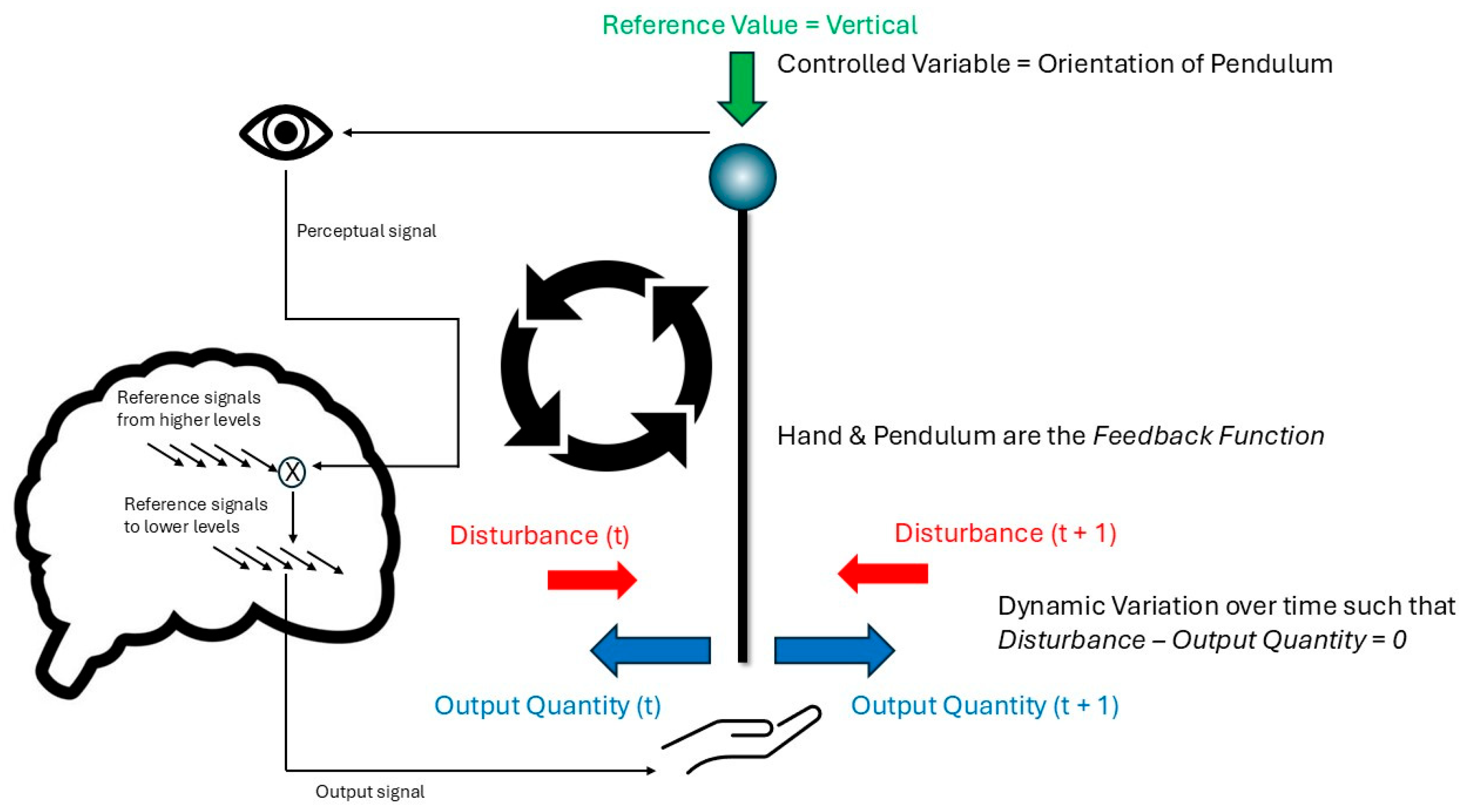
Figure 1.
The closed loop of PCT in the case of balancing an inverted pendulum. The diagram illustrates the dynamic variation in hand movement at the bottom of the pole to counteract disturbances to the vertical orientation of the pole, so that the pole is kept close to constantly vertical—the reference value. The source of control comes from higher level control systems in the agent, whose reference values are subtracted from incoming perceptual signals during this task (via the comparator illustrated by a cross in a circle; only one is illustrated for simplicity). The subtraction leads to an error signal that sets lower-level signals for outputs to the muscles of the arm and hand. The diagram is designed to illustrate that this loop is a continuous process that occurs during the performance of this behavior—balancing a pendulum—even in the absence of any learning.
Figure 2.
A control unit based on PCT. Reproduced with permission from Dag Forssell. Note: The figure shows the specific components of the closed loop in PCT. Inside the agent, a reference signal specifies the desired magnitude of the perceptual signal, which represents the current magnitude of one aspect of the environment (or self) to be controlled; this is known as the controlled variable (CV); for example, it could be the distance from a target destination. Each aspect of the environment is constructed from an input function, which transforms and integrates signals from lower levels to form the perceptual signal. The difference between the reference signal and perceptual signal is the error signal, which is transformed by the output function within the agent to act through the environment (via the feedback function) to counteract disturbances in the environment that affect the input quantity of the controlled variable.
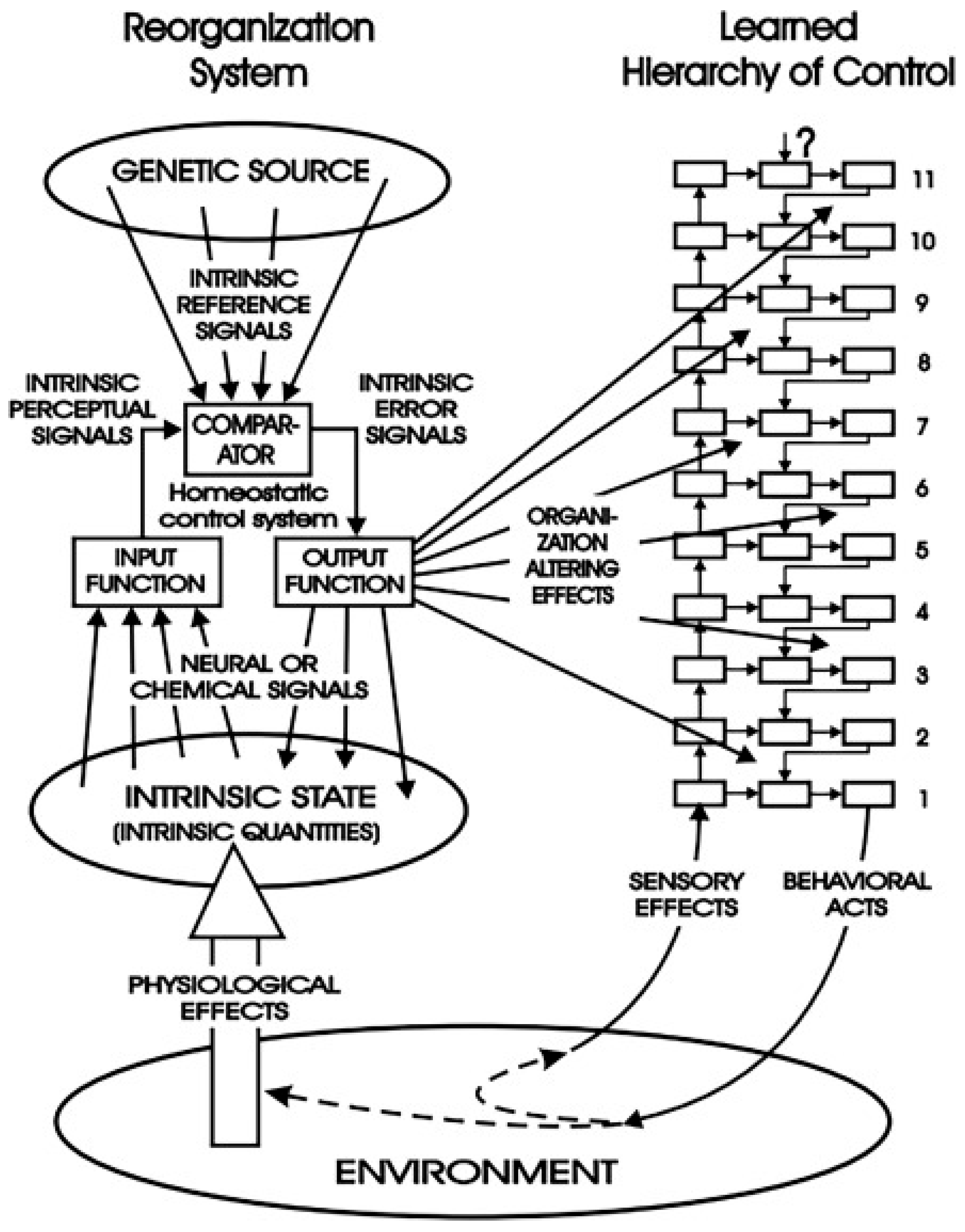
Figure 3.
The reorganization system of intrinsic variables and its relation to the learned hierarchy in PCT. The perceptual hierarchy defines and implements goal-directed behavior, whereas the reorganization system prompts trial-and-error changes in the parameters (e.g., gains) of the perceptual hierarchy when intrinsic variables shift from their reference values. Reproduced with permission from Living Control Systems Publishing.
Figure 4.
An analogy illustrates how the identity of objects depends on their distinguishability, which itself depends on some degree of causal separation. Here, each liquid is a different “object”, while the divider represents the degree of causal separation. The more holes in the divider, the smaller the degree of separation, and the faster the two “objects” become one, an indistinguishable object.
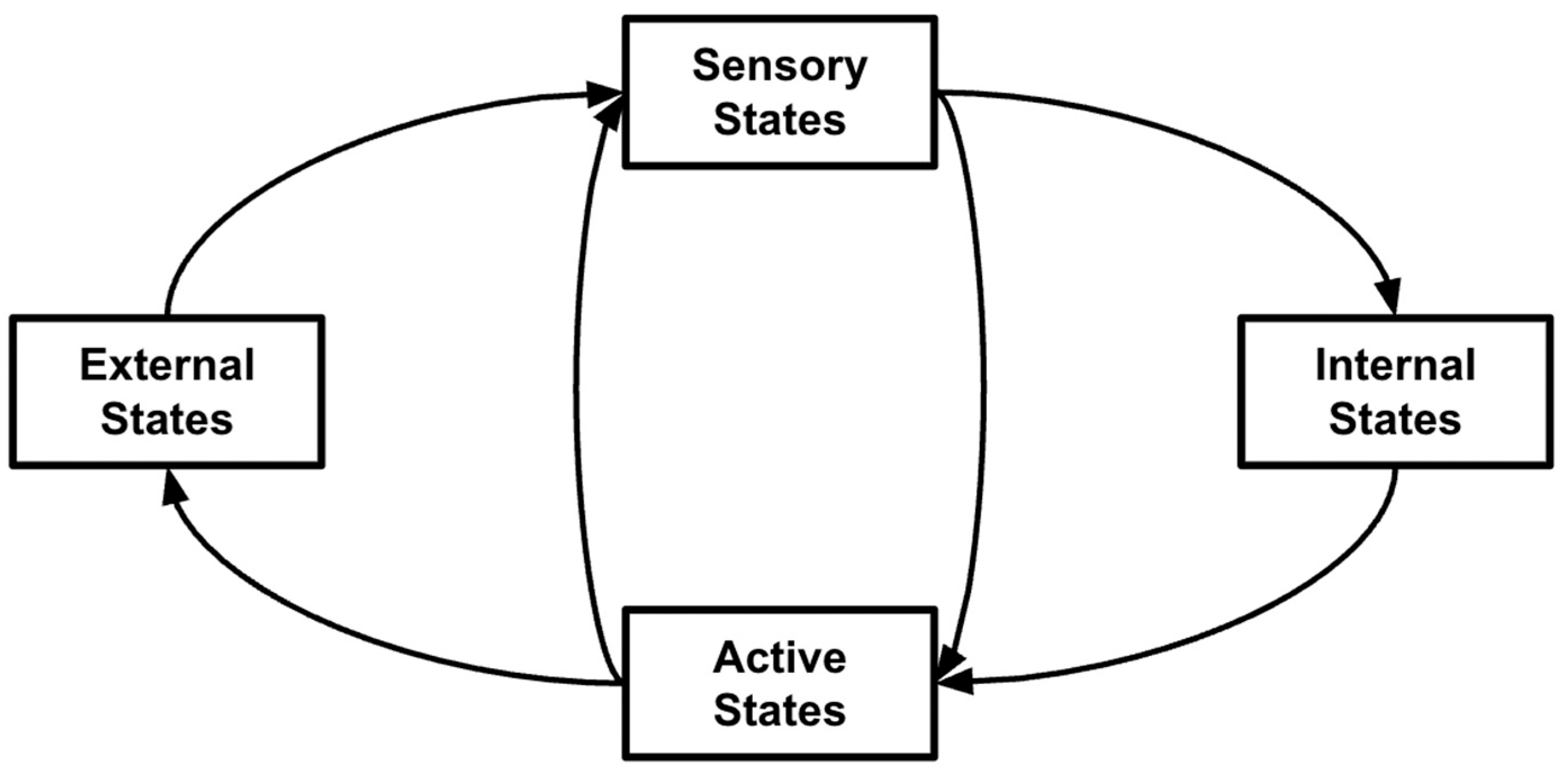
Figure 5.
Figure illustrating the Markov blanket construction broadly, where external states constitute the environment while internal states constitute organismal variables that are causally separated from the environment, given sensory and active states. The sensory and active states constitute the Markov blanket mediating interaction between the environment and the agent.
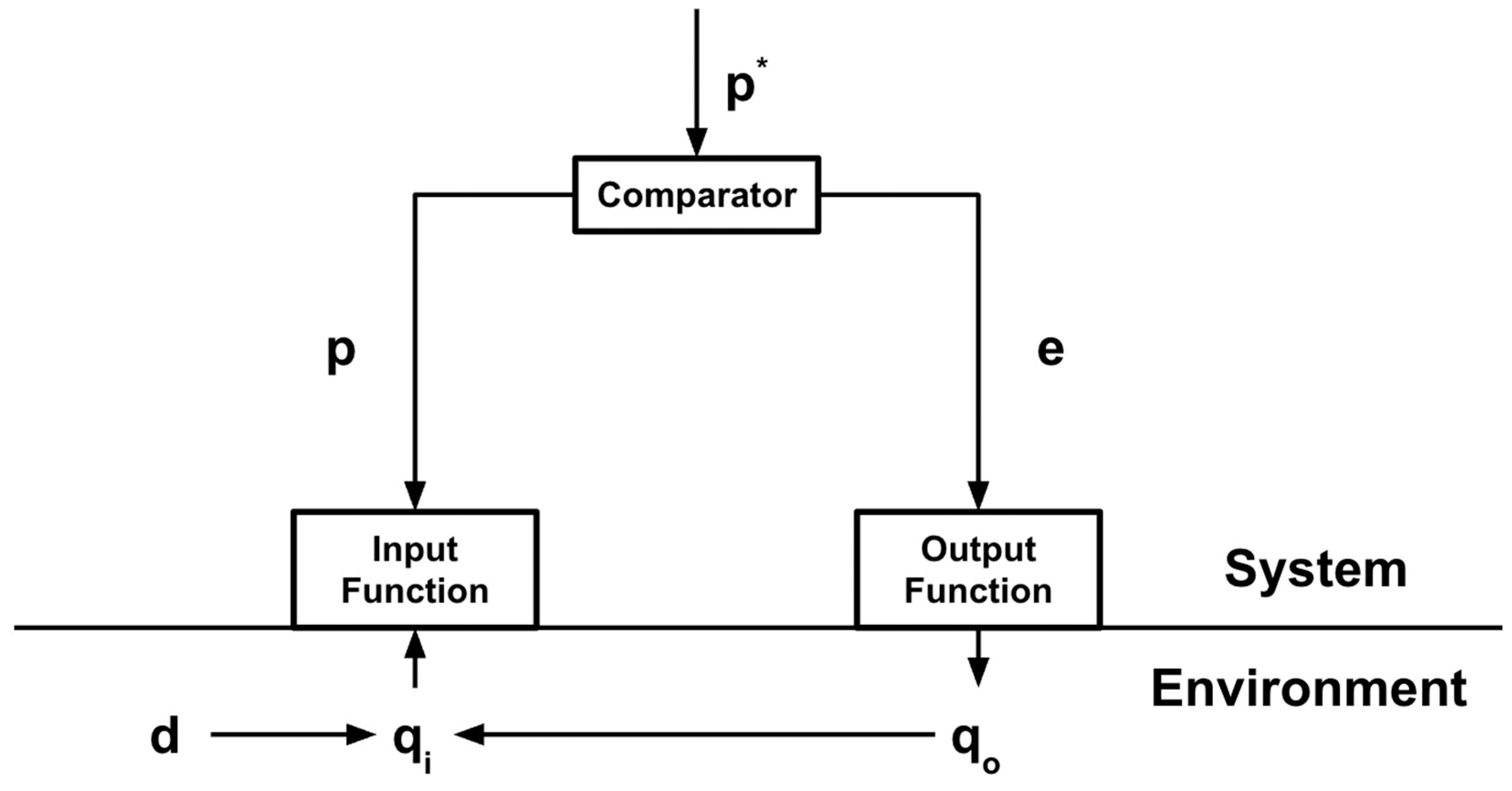
Figure 6.
A simplified reproduction of
Figure 2, showing a control unit based on PCT. From the diagram we have,
qi that represents the actual environmental stimulus, like light, or sound;
p for the “representation” of the environmental stimulus (
qi) produced by the input function—known as the perceptual signal; d that represents a disturbance to the environmental stimulus (
qi) produced by environmental factors, like an obstacle that blocks one’s view, or earmuffs that block one’s sense of hearing;
p* for the internal reference signal, or signals, generated by the organism; and e for the error generated by the comparator after comparing both the representation of the environmental stimulus (
p) and the internal reference signal (
p*).
Figure 7.
An image from a visualization of a PCT E. coli model’s trajectory to the target attractant. The red dot indicates the position of the E. coli. The yellow dot indicates the position of the target. The green trail indicates the path taken by the E. coli. The blue boundary represents the start of the area in which “food” is accumulated.
Figure 8.
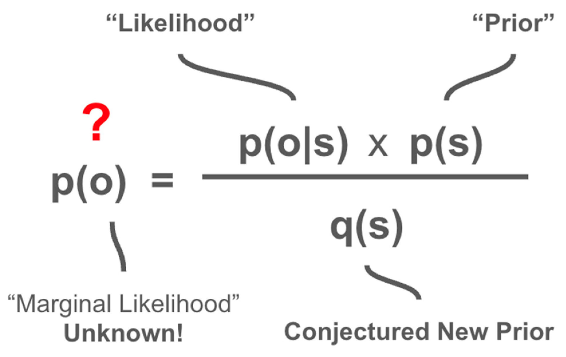
The equations for the exact form of Bayesian Inference are where , or the “posterior”, quantifies the optimal new beliefs about hidden state “s” after one observes an event, or “evidence”, which is denoted “o” for “observations”. In English, this is usually read “the probability of the hidden state given the observations”. In contrast, —is the “probability of observations given the hidden state”. This is called the “likelihood” and is an inversion of the posterior. Therefore, the likelihood quantifies beliefs about what hidden states are most likely to cause a particular observation. are “prior”, or current beliefs about the hidden state, while , also called the “marginal likelihood” of the observation—that is, the probability that a particular observation will occur, averaged over all possible hidden states according to their prior probabilities (). Importantly, while , , and are 1-Dimensional Probability Distributions, is matrix such that the product of and is the joint probability distribution which is referred to as the agent’s “generative model”.
![Foundations 05 00035 g008 Foundations 05 00035 g008]()
Figure 9.
Rearrangement of Bayes’ Theorem to reflect an unknown, or intractable marginal likelihood.
Figure 9.
Rearrangement of Bayes’ Theorem to reflect an unknown, or intractable marginal likelihood.
Figure 10.
This figure illustrates the discretization of the perceptual signal into buckets that faithfully represent the difference between the angle the E. coli is facing and the angle between the E. coli and the target. The code reproducing the figure can be found attached to this article.
Figure 10.
This figure illustrates the discretization of the perceptual signal into buckets that faithfully represent the difference between the angle the E. coli is facing and the angle between the E. coli and the target. The code reproducing the figure can be found attached to this article.
Figure 11.
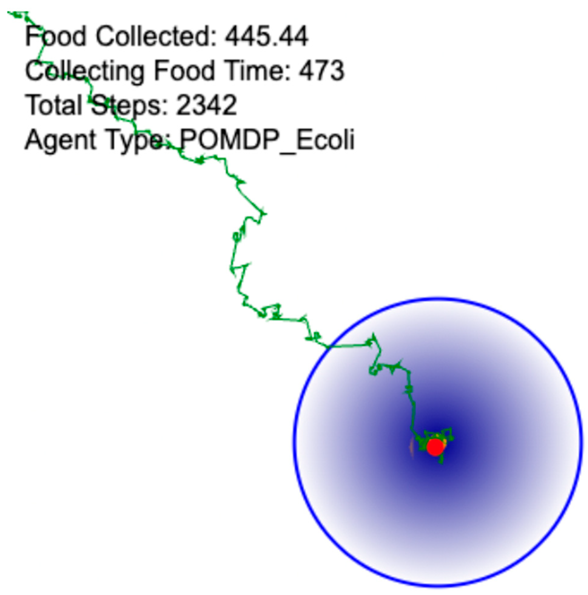
A trajectory of a POMDP E. coli model towards the center of a target attractant.
Figure 11.
A trajectory of a POMDP E. coli model towards the center of a target attractant.
Figure 12.
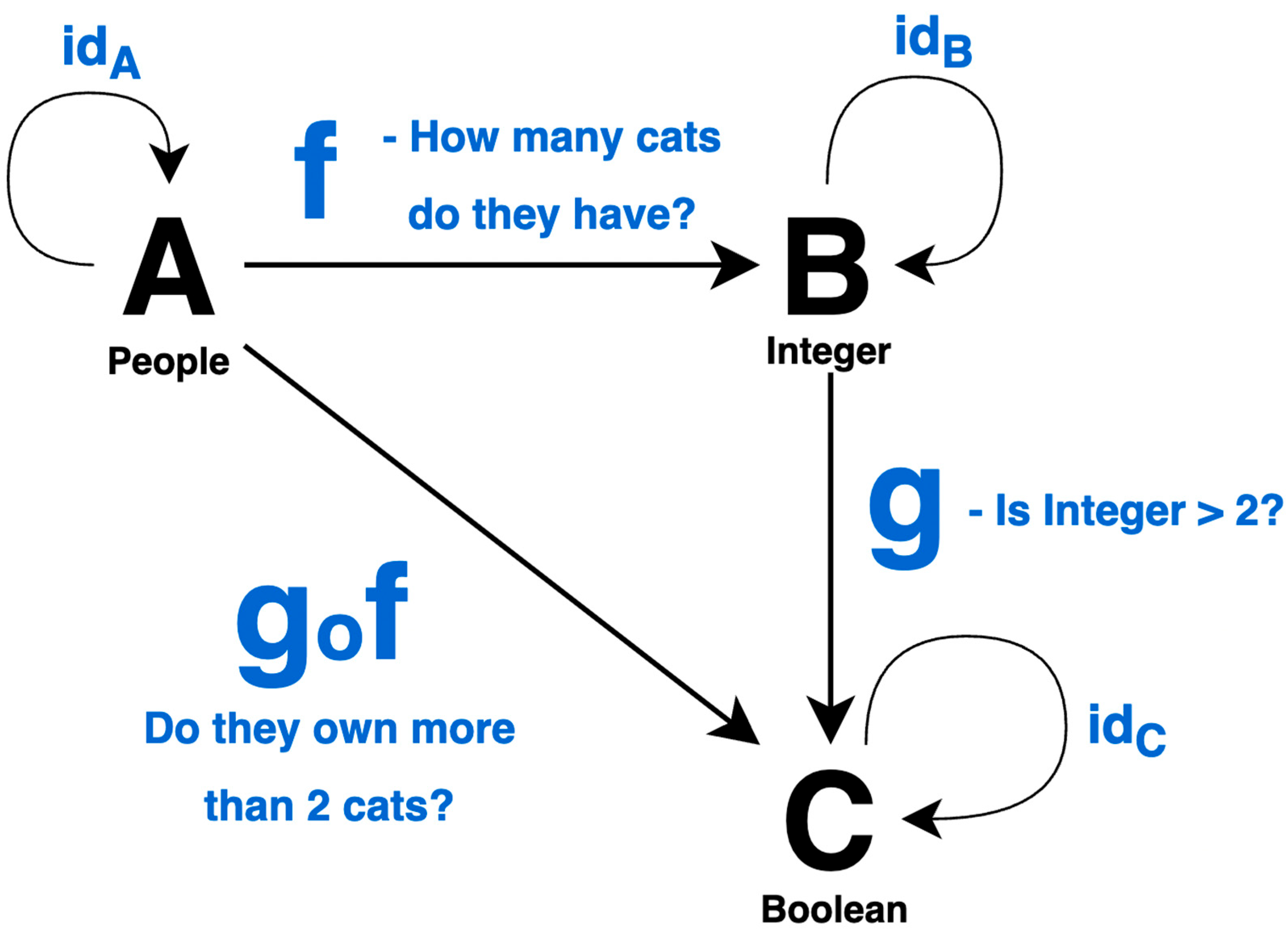
Diagram of a simple category where all morphisms have blue labels that describe how they map their source and target objects. The diagram includes identity morphisms for each object, which are normally not drawn.
Figure 12.
Diagram of a simple category where all morphisms have blue labels that describe how they map their source and target objects. The diagram includes identity morphisms for each object, which are normally not drawn.
Figure 13.
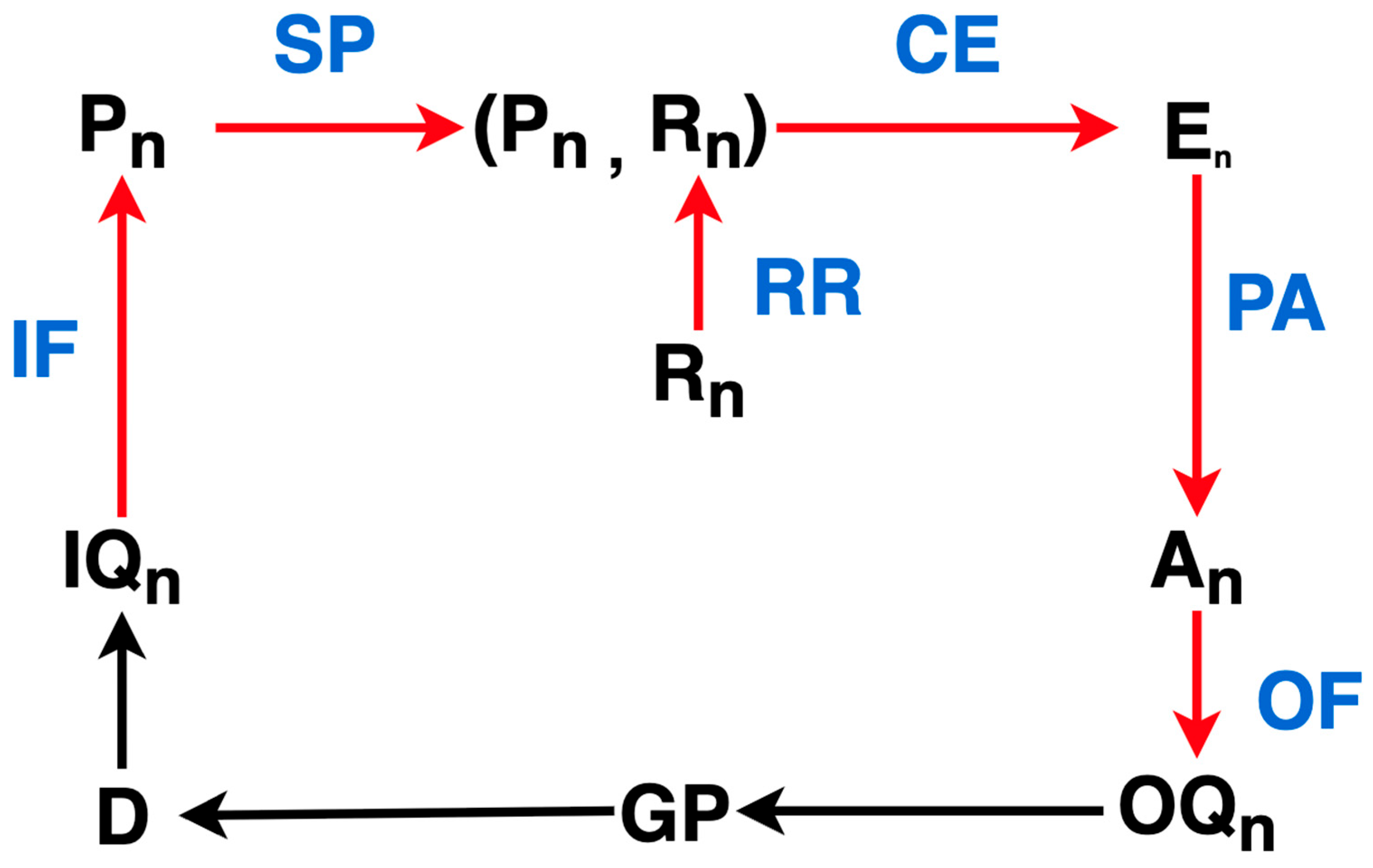
The PCT Agent Category. Morphisms that are internal to the category, that is, actually modeled explicitly by the PCT paradigm, are colored in red. Black morphisms indicate morphisms whose function may not be known and are located in the “environment category”. The blue symbols are the abbreviated names of all morphisms internal to the category which are not necessarily named as such in the literature.
Figure 14.
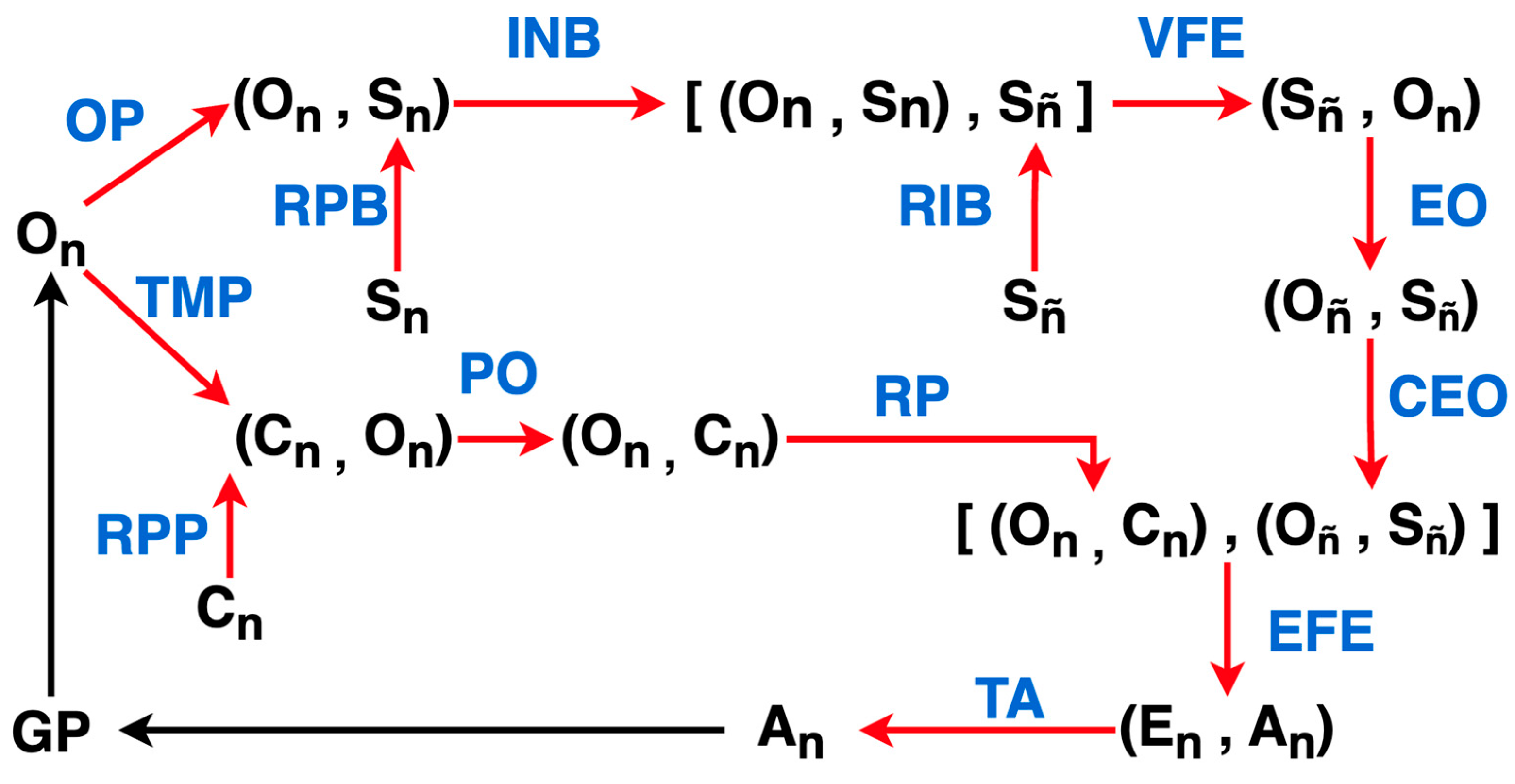
The FEP Agent Category. Morphisms that are internal to the category, that is, actually modeled explicitly by the FEP paradigm, are colored in red. Black morphisms indicate morphisms whose function may not be known and are located in the “environment category”. The blue symbols are the abbreviated names of all morphisms internal to the category, which are not all necessarily named as such in the literature.
Figure 15.
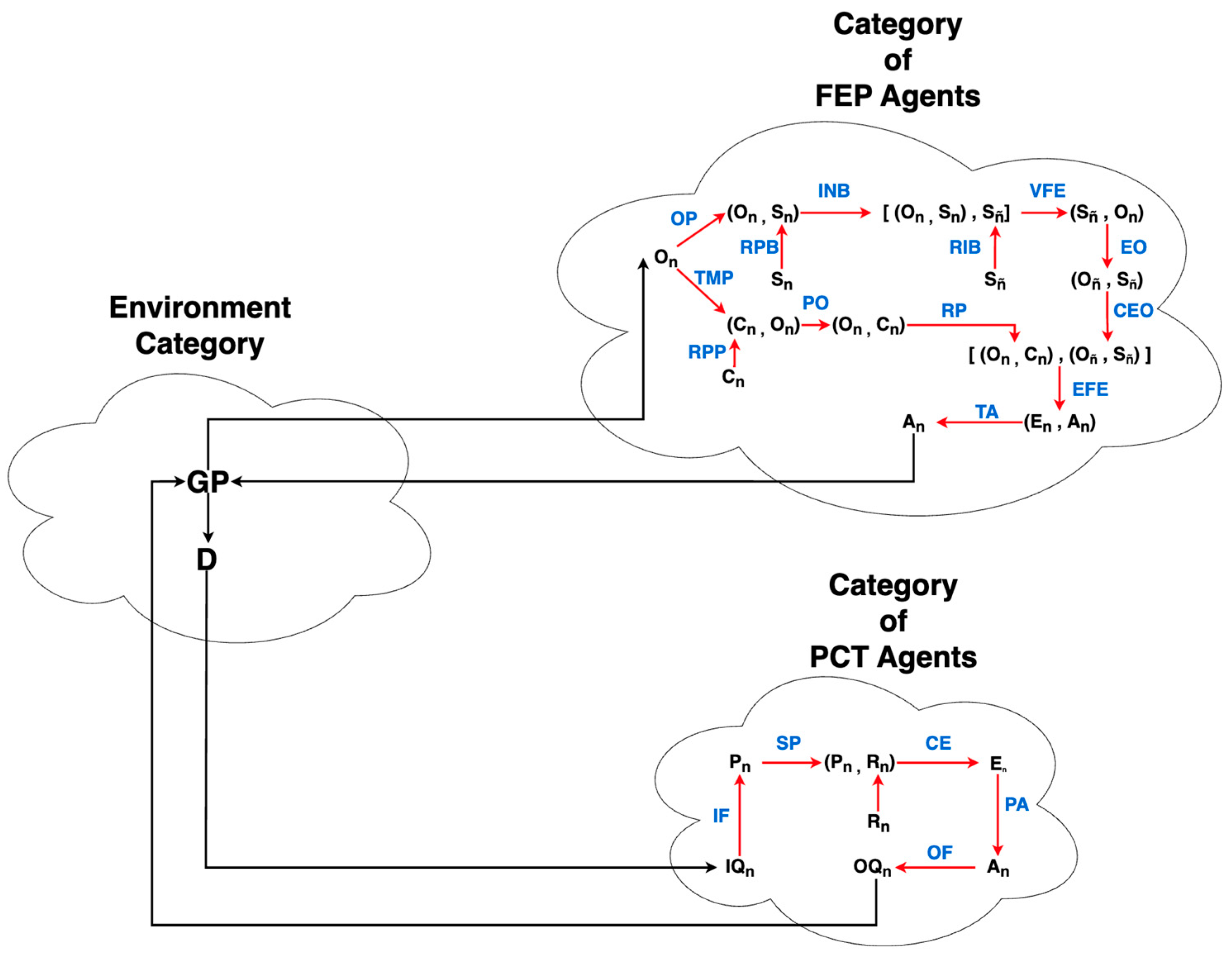
A diagram representing how one would couple interactions between PCT and FEP agents. The environment that affects the input quantity
Figure 15.
A diagram representing how one would couple interactions between PCT and FEP agents. The environment that affects the input quantity
Figure 16.
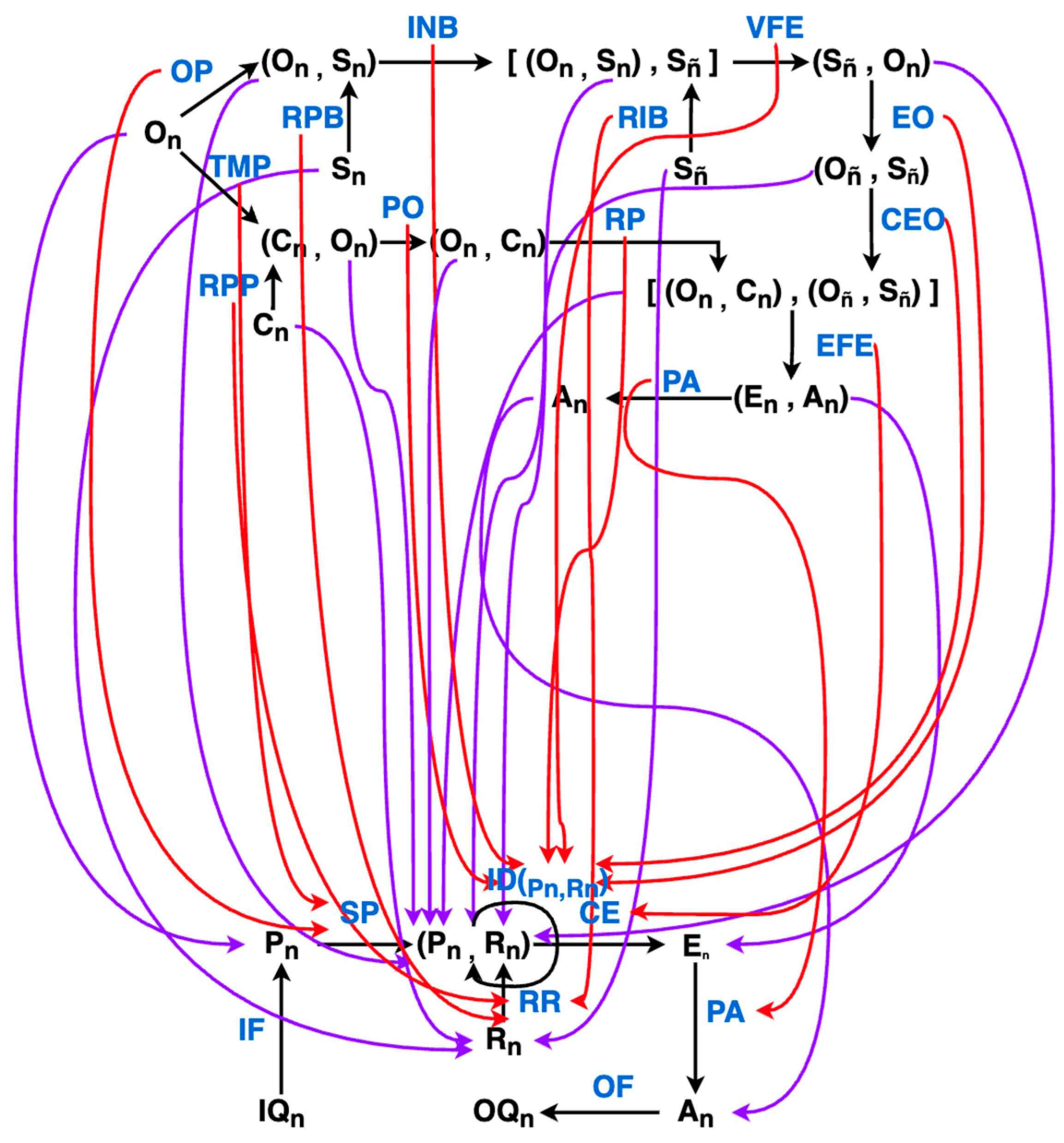
The functor. Here, morphisms internal to categories are black. The functor consists of mappings from objects and morphisms in the FEP category to objects and morphisms in the PCT category. Environmental morphisms and their associated objects have been removed from the diagram for clarity.
Figure 17.
An illustration of the Internal Variable Subfunctor. Here, the source objects of each morphism in each subcategory correspond to the parameters of that agent category. In this case, the prior , approximate new prior distribution and log prior preference are FEP parameters, while PCT parameters consist only of the reference variable . The target objects are outputs of the operations represented by their respective morphisms.
Figure 18.
An illustration of the Perception Action Subfunctor. Here, each of the subcategories consists only of objects and morphisms corresponding to how perception is received and how action is performed.
Figure 18.
An illustration of the Perception Action Subfunctor. Here, each of the subcategories consists only of objects and morphisms corresponding to how perception is received and how action is performed.
Figure 19.
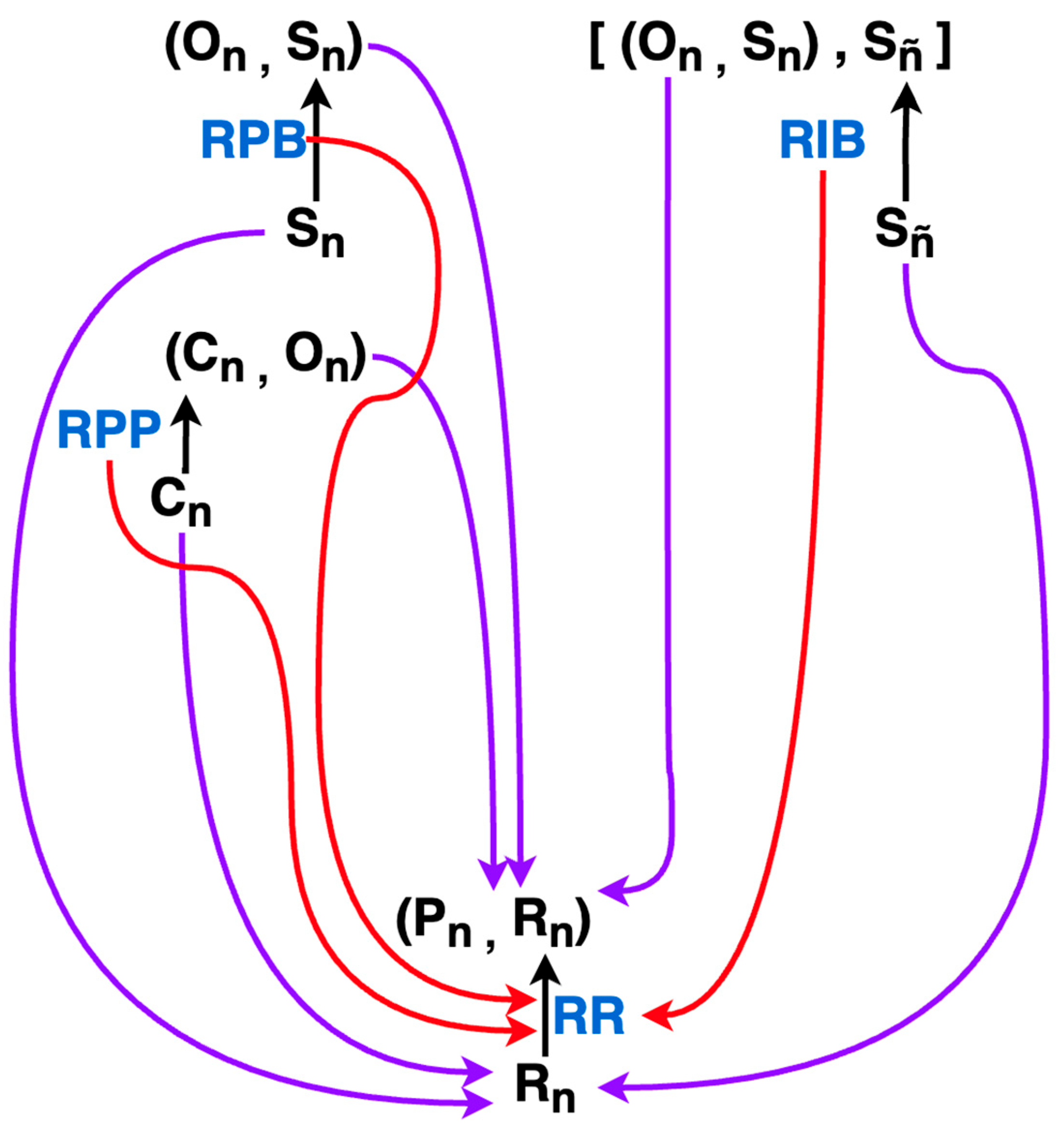
An illustration of the Uncertainty–Certainty Subfunctor. Here, each of the subcategories consists only of objects and morphisms concerned with how integrated perceptions are prepared such that they can drive action.
Figure 19.
An illustration of the Uncertainty–Certainty Subfunctor. Here, each of the subcategories consists only of objects and morphisms concerned with how integrated perceptions are prepared such that they can drive action.
Figure 20.
An illustration of the distribution of average distance from the center and the ratio of time spent collecting food for 2880 different PCT E. coli Model Parameters.
Figure 20.
An illustration of the distribution of average distance from the center and the ratio of time spent collecting food for 2880 different PCT E. coli Model Parameters.
Figure 21.
An illustration of the distribution of average distance from the center and ratio of time spent collecting food for 2880 different FEP E. coli Model Parameters.
Figure 21.
An illustration of the distribution of average distance from the center and ratio of time spent collecting food for 2880 different FEP E. coli Model Parameters.
Figure 22.
An illustration of a functor from a “Category of Hodgkin–Huxley Neurons” to the PCT Agent Category is illustrated in Figure N. For brevity, only object mappings for the functor are pictured. Many of these morphism mappings can be inferred given their source and target object mappings. When source and target objects are mapped to the same object in the target category, the morphism between them must be mapped to the identity of that target object. Note that is the total electrical state of the cell, which maps to a pair of the change in voltage and current voltage with the following morphism: . This is isomorphic with the composite morphism in the PCT category: . In other words, the total electrical state of the neuron is its output quantity, and the voltage of the cell is its input quantity.
Table 1.
This table summarizes the PCT E. coli model algorithm. The variables and parameters are defined.
Table 1.
This table summarizes the PCT E. coli model algorithm. The variables and parameters are defined.
| Step | Algorithm | Description |
|---|
| 1 | x := x + v · cos(a)
y := y + v · sin(a) | Swim a fixed distance v in the current heading a. |
| 2 | φ := atan2(yₜ − y, xₜ − x) | Compute the angle φ to the attractant source. |
| 3 | | Input function: convert motion through the gradient into a perceptual signal p (temporal derivative of concentration). |
| 4 | e := p* − p | Comparator: difference between reference p* and perception p. |
| 5 | dq := K·e | Output function: convert error to the increment dq of an internal “messenger” substance. |
| 6 | q := q + dq | Accumulate the substance. |
| 7 | if q > Q then
q := 0
a := random(0, 2π) | When accumulation exceeds threshold Q, trigger a tumble (pick a new heading uniformly at random). |
p, p*, e—same as previously defined; v—velocity that the E. coli can move at—Kept Fixed; a—angle that the E. coli is heading; G—scaling constant for the perceptual signal—Kept Fixed; K—scaling constant for the error function; dq—Increment of accumulated “substance”; q—total “substance” accumulated; Q—tumble threshold; Φ—angle to the target, or attractant source; (xₜ, yₜ)—location of the target; (x, y)—location of the E. coli.
|
Table 2.
Log preferences for each possible label in the model. Note: While preferences are expressed as a vector, they are not probability distributions; therefore, their values need not sum to 1 or be bounded between 0 and 1. This is because preferences do not encode beliefs about the world but rather reflect relative desirability. For example, a preference vector like [−10, 0, 5] implies that state 0 is strongly avoided, state 1 is neutral, and state 2 is highly preferred. What matters are the relative magnitudes, not absolute probabilistic interpretations.
| Observation Label | Log Preferences |
|---|
| 0–120 | 0.00 |
| 120–140 | −8.48 |
| 240–360 | −8.48 |
Table 3.
Probability values for each hidden state in the prior —each with an equivalent value, which maximizes the entropy of the distribution and can be interpreted as having no bias towards being some distance away from the target.
Table 3.
Probability values for each hidden state in the prior —each with an equivalent value, which maximizes the entropy of the distribution and can be interpreted as having no bias towards being some distance away from the target.
| State Label | Prior State Probability |
|---|
| Near (to target) | 33% |
| Mid (from target) | 33% |
| Far (from target) | 33% |
Table 4.
The likelihood matrix, which details the probability of being near, mid, or far from the target given the observed angle between the agent and the target. This can be interpreted as having sharp biased beliefs, where the agent believes it is near the target with 100% certainty if the angle it observes is 0–120.
| | Near (to Target) | Mid (from Target) | Far (from Target) |
|---|
| 0–120 | 100% | 0% | 0% |
| 120–140 | 0% | 100% | 0% |
| 240–360 | 0% | 0% | 1.00% |
Table 5.
Transition Matrix “Part 1” that defines the probability of the next state given the previous state and the action taken. In this case, the action being taken is “approach”—Therefore, this can be interpreted as the agent believing that if it is near the target, then “approach” will result in being near with a 90% probability.
| | Near (to Target) | Mid (from Target) | Far (from Target) |
|---|
| Near (to target) | 90% | 5% | 0% |
| Mid (from target) | 10% | 90% | 10% |
| Far (from target) | 0% | 5% | 90% |
Table 6.
Transition Matrix “Part 2”. In this case, the action being taken is “tumble”. Therefore, this can be interpreted as the agent having no biased beliefs about where it will be in relation to the target after tumbling.
Table 6.
Transition Matrix “Part 2”. In this case, the action being taken is “tumble”. Therefore, this can be interpreted as the agent having no biased beliefs about where it will be in relation to the target after tumbling.
| | Near (to Target) | Mid (from Target) | Far (from Target) |
|---|
| Near (to target) | 33% | 33% | 33% |
| Mid (from target) | 33% | 33% | 33% |
| Far (from target) | 33% | 33% | 33% |
Table 7.
“hi” corresponds to high probability mass, which is equal to the likelihood sharpness. “lo” corresponds to low probability mass and is calculated with the following function: This results in a proper probability matrix where rows sum to 1.
Table 7.
“hi” corresponds to high probability mass, which is equal to the likelihood sharpness. “lo” corresponds to low probability mass and is calculated with the following function: This results in a proper probability matrix where rows sum to 1.
| | Near (to Target) | Mid (from Target) | Far (from Target) |
|---|
| 0–120 | hi | lo | lo |
| 120–140 | lo | hi | lo |
| 240–360 | lo | lo | hi |
Table 8.
This illustrates how the nonlocality bias is used as a scalar hyperparameter to tune the transition matrix for the “approach” action of the model.
Table 8.
This illustrates how the nonlocality bias is used as a scalar hyperparameter to tune the transition matrix for the “approach” action of the model.
| | Near | Mid | Far |
|---|
| Near | | | 0% |
| Mid | | | |
| Far | 0% | | |
Table 9.
This illustrates how the log prior preference vector was encoded with a single scalar hyperparameter.
Table 9.
This illustrates how the log prior preference vector was encoded with a single scalar hyperparameter.
| Observation Label | Log Preferences |
|---|
| 0–120 | 0.00 |
| 120–140 | log(x) |
| 240–360 | log(x) |
