Abstract
This study investigates the origin and amplification of magnetic fields in planets and galaxies, emphasizing the foundational role of a seed magnetic field (SMF) in enabling dynamo processes. We propose a universal mechanism whereby an SMF arises naturally in systems where an orbiting body rotates non-synchronously with respect to its central mass. Based on this premise, we derive a general equation for the SMF applicable to both planetary and galactic scales. Incorporating parameters such as orbital distance, rotational velocity, and core radius, we then introduce a dimensionless factor to characterize the amplification of this seed field via dynamo processes. By comparing model predictions with magnetic field data from the solar system and the Milky Way, we find that the observed magnetic fields can be interpreted as the product of a universal gravitationally induced SMF and a body-specific amplification factor. Our results offer a novel perspective on the generation of magnetic fields in a wide range of astrophysical contexts and suggest new directions for theoretical investigation, including the environments surrounding black holes.
1. Introduction
Magnetic fields are a ubiquitous feature of the Universe, observed across a wide range of structures, i.e., from planets and stars to galaxies, clusters of galaxies and interstellar and intergalactic space (e.g., [1,2,3,4,5]).
These fields are generally understood to arise from two components: a seed magnetic field (SMF) and an amplified dynamo field (DF). The SMF is a necessary precursor, as the dynamo process requires an initial magnetic field to initiate and sustain amplification through internal conductive motions (e.g., [6]).
The concept of an SMF is context-dependent and varies across the hierarchy of cosmic of cosmo-magneto-genesis (e.g., [7,8,9]). It may refer to a primordial SMF generated during cosmic inflation [10,11], or to more localized seed fields arising during galaxy or planetary formation.
While many cosmological models have been proposed, including inflationary and post-inflation scenarios (e.g., [12]), these approaches often face difficulties such as insufficient coherence scales or physical constraints from gravitational wave production and Big Bang nucleosynthesis [3]. For instance, second-order photon–electron interactions during the epoch of recombination have been proposed as possible origin of early cosmic magnetic fields.
In this paper, however, we focus on SMFs generated at the scale of planetary systems, which could cumulatively influence galactic-scale magnetism. Accordingly, we do not consider early-universe mechanisms in detail [11] but instead concentrate on later-stage processes that occur once orbital systems have formed.
Several hypotheses have been advanced to explain SMF generation at planetary and galactic scales:
- (i)
- Remnant interstellar magnetic fields: During the collapse of the protoplanetary disk, magnetic fields from the interstellar medium could be “frozen in” and carried into the forming planet [10,13].
- (ii)
- Solar nebula fields: The magnetic field of the early Sun could have permeated the protoplanetary disk and implanted a seed field in the forming planetary body [14].
- (iii)
- Impact-generated fields: Large-scale impacts during accretion might briefly generate magnetic fields via shock-induced ionization and local dynamos (e.g., [15,16]).
- (iv)
- Thermoelectric effects: Inhomogeneities in temperature and composition during core formation might generate small-scale fields (e.g., [17]).
However, each of these sources comes with challenges regarding strength, coherence, and survivability of the field during the high-temperature, turbulent formation processes of planetary interiors (e.g., [18,19]).
Planetary magnetic fields observed today, such as Earth’s, are sustained by dynamo action—specifically α2 or αω dynamos—which generate large-scale poloidal fields through the motion of electrically conductive fluid in a rotating planetary core (e.g., [6,20]). Yet, this process requires a pre-existing SMF to begin. The origin of this seed field remains uncertain and is referred to as the primordial magnetic field problem [21].
Once a weak SMF is present, the dynamo can exponentially amplify it, provided conditions such as sustained convection and differential rotation are met. Importantly, the characteristics of the seed field can influence the early geometry and strength of the evolving magnetic field.
In this work, we propose a novel hypothesis: a universal SMF naturally arises in systems where a rotating body orbits a central mass with non-synchronous rotation. Based on fundamental thermodynamic and gravitational principles, we derive a general expression for this SMF and apply it across both planetary and galactic scales. We further explore how this seed field may be amplified through internal dynamo processes by introducing a dimensionless formulation to compare theoretical predictions with observational data.
Our goal is to unify the understanding of magnetic field origins through a model that bridges gravitational dynamics and internal fluid motion. While this mechanism may not be directly applicable to early-universe or large-scale cosmological structures, we argue that it is particularly suited, under certain conditions, to localized orbiting systems, such as planets, satellites, and possibly stars, accretion disks, galaxies, spiral galaxies, and collimated relativistic jets, where an 1/r decay of the magnetic field could be possible [7,22,23,24]. Our hypothesis is intended to complement, rather than replace, existing dynamo theories, offering a new perspective on the initial magnetic conditions necessary for their activation.
All the acronyms and physical quantities used throughout this article are defined in Appendix A.
2. Magnetic Field of Our Galaxy
The magnetic field of the Milky Way has been extensively studied through radio observations and Faraday rotation measures [25]. An intriguing feature of our galaxy is given by [22]. Figure 1 shows the observed radial profile of the galactic magnetic field (blue line); overlaid are comparative trends that represent theoretical field decays with distance. It is quite evident how the total field (blue line) of the Galactic magnetic field B has a trend that is very close to 1/r (red line), rather than 1/r2 (black line) and the “classic dipolar” 1/r3. Therefore, any distributions of monopoles or dipoles (following the 1/r2 trend or 1/r3 trend, respectively) cannot explain the observed overall galactic magnetic field. The persistence of a 1/r profile at large galactic radii motivates our hypothesis that a universal seed magnetic field (SMF), independent of internal dynamos, contributes to the observed field. This SMF may arise from the orbital and rotational dynamics of celestial bodies—a hypothesis that we formalize in the following section.
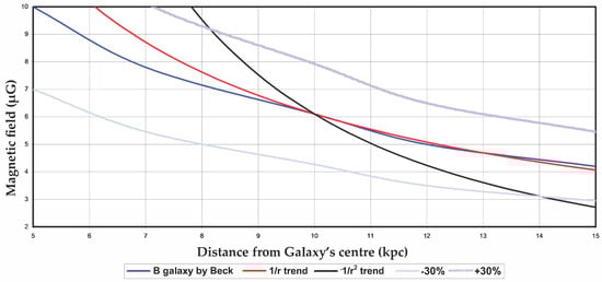
Figure 1.
Radial dependence of the Galactic magnetic field (blue curve; as deduced from [22]), compared with hypothetical decay profiles: 1/r (red), and 1/r2 (black).
3. The Seed Magnetic Field (SMF)
Current theories consider three stages for the magnetic field formation in galaxies (e.g., [26]): (i) a seed field generated in the early Universe; (ii) a small-scale dynamo, which efficiently amplifies the field through turbulence in the gas driven by supernova explosions or spiral shocks; and (iii) a final and most time-consuming stage, which involves the ordering of the turbulent field.
For ease, we now adopt the simplified hypothesis that the present magnetic field of planets or galaxies arise from two contributions: the SMF and the DF, with the latter including the stages (ii) and (iii), while the former does not necessarily need to occur in the early Universe, but it could appear even in a later stage, i.e., during the formation of planetary systems.
Our original and innovative hypothesis is that the SMF can be universally generated by the non-synchronous orbital and rotational motion of a body around a central mass (although we do not exclude its generation by means of other known mechanisms [26]). The DF arises from internal convective motions that amplify the SF. Therefore, the DF needs the SMF to be activated: it is like a thermodynamic engine that needs a start motor to begin working. From Figure 1, it is clear that the effect of the SMF is still present at large scales, producing the 1/r trend at galactic level. Therefore, what we observe at planetary system and galactic scales is the reminiscence of that field.
In this section, we focus on deriving a general expression for the SMF from fundamental principles.
Consider a celestial body of mass m, in thermodynamic equilibrium, orbiting a central mass along circular paths with constant angular velocity ω, while also rotating around its own axis—perpendicular to the ecliptic plane—with constant angular velocity ω1.
Under the assumptions of weak gravitational fields (distances r >> rg) and velocities much lower than the speed of light, and assuming that H is the only electromagnetic field, aligned with the body’s axis of rotation and dependent solely on the radial distance r, a simplified energy-based argument yields a differential scalar relation involving the magnetic field (see the Appendix B for more details).
The resulting equation is:
(Please recall that B = μ0H in the vacuum).
Equation (1) can be integrated in the case where ω ≠ ω1; otherwise, we would reduce to a trivial equation like 0 = 0). Therefore, for ω ≠ ω1, we have the following non-trivial solution (The latter is a good approximation except in the vicinity of the couples of bodies) (see Appendix C):
where k is a constant dependent on the orbital and physical parameters of the system, and rg is the gravitational radius of the central mass. This latter quantity is the Schwarzschild theoretical radius to which the central mass would need to be compressed to collapse into a BH; for the Sun is only about 3 km (e.g., [27]). The solution (2) exhibits a 1/r for large r, consistent with observational data (see Figure 2).
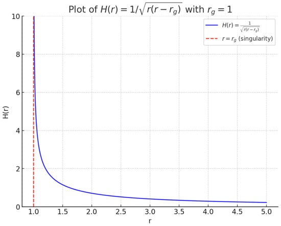
Figure 2.
Expression of the magnetic field H of (2) with respect to the distance r; rg is considered as unitary, for convenience.
This expression suggests that the SMF is a gravitationally induced magnetic field, emerging from the differential motion between a rotating body and its orbit (Figure 3). Unlike traditional dipolar or multipolar sources, this field does not require an internal conducting fluid for its origin—though such a medium is still necessary to amplify it via the dynamo effect.
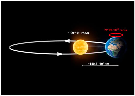
Figure 3.
A body orbits rotating non-synchronously around a larger body, such as a star, e.g., the case of Earth around the Sun. The angular velocities ω and ω1 are shown for Earth, together with the Sun–Earth distance.
Importantly, this formulation generalizes and extends earlier ideas—such as those of Blackett [28,29]—by directly linking the magnetic field to rotational dynamics in a broader astrophysical framework. Our hypothesis is not restricted to planetary scales, but may also apply to stars, accretion disks, and galactic structures.
Figure 2 and Figure 3 illustrate the behavior and origin of the SMF: a body orbiting a central mass with non-synchronous rotation naturally develops a weak magnetic field with a 1/r spatial dependence. This field provides the initial condition required for dynamo amplification.
For the Solar System our relativistic corrections are numerically negligible: for the Sun rg≃2.95 km, so at Earth’s orbit rg/r∼2 × 10−8 (even smaller at larger radii), and therefore Newtonian gravity is entirely adequate for the numerical comparisons in next Section 5 and Section 6. However, we retain the (simple) Schwarzschild-language here for two reasons: (i) it makes explicit the role of the gravitational redshift (the lapse α2 = 1 − rg/r) in relating locally measured field energy to the conserved Killing/Hamiltonian energy, and (ii) it permits immediate generalization to compact-object environments (e.g., black holes and inner accretion-disk regions), where α deviates significantly from unity and relativistic effects are essential.
4. Qualitative Observations
An important observation is that the presence of a liquid or gaseous electrically conductive core in the orbiting body can give rise to electric currents, which are likely responsible for the dynamo mechanism that amplifies the SMF and then sustains the planetary magnetic field. To explore the relationship between the SMF, as deduced from (1), and the magnetic field generated by the dynamo effect it triggers, we propose the following qualitative observations:
- There are several ways to express the dynamo effect (e.g., [30,31,32]). However, we can use a very simplified expression that can be seen as a multiplicative factor of the SMF itself: , where
- In a planet we expect that the dynamo effect is somehow linked to the surface available for the passage of the current and therefore proportional to , where Rc represents the radius of the liquid core of the planet.
- We also assume a proportionality with respect to the non-synchronous part of the angular velocity, and therefore to , since the higher this parameter is, the greater the energy available to generate the magnetic field.
- Instead, an inverse proportionality to the distance from the central body is expected. This is because Equation (2) suggests a link between magnetism and the gravitational field governing the planet’s orbit, a link that weakens with the increasing distance.
- Another qualitative aspect that we expect to find is that, when , we have that , quickly enough due to the presence of increasingly important resistances to the circulation of the current.
- Conversely, we expect that for we have that , where is a finite value since the energy involved in making the current flow is finite in any case.
These qualitative principles will guide the construction of a dimensionless amplification function, introduced in the next section. The goal is to bridge planetary properties (such as core size, angular velocity, and orbital distance) with the observed magnetic field strengths, using a unified scaling model.
5. Dimensionless Parameters and Mathematical Formulation
Building on the qualitative considerations introduced in the previous section, we now construct a quantitative framework to describe the amplification of the SMF by internal dynamo processes. Our goal is to express the total magnetic field as function of a small set of physically meaningful parameters, allowing comparison across planetary and galactic systems.
We introduce a dimensionless parameter α that takes into account the previous points II, III and IV, in the simplest way, as
where represents the speed of light. Here, is a dimensionless dynamo efficiency factor related to the geometry and energy budget of the core [2]. Once is defined, we can find the relation that satisfies the previous points V and VI. This relation is the following:
The adimensional parameters γ, δ must be chosen to interpolate the available data.
In order to compute those parameters γ, δ, let us follow the next step by step procedure, starting from our solar system.
6. Curve Fitting for Planets and Satellites
To evaluate the model quantitatively, we calibrate the parameters using observational data from planetary bodies. First, we determine the constant k in Equation (2) using a reference planet where the dynamo effect is negligible, for example, Venus, exhibits an extremely weak magnetic field despite having a sizeable core [19]). For this assumption, we derive:
This establishes a reference SMF in the absence of amplification. Actually, since we expect that , we should get
Next, we compute the total field strength for other celestial bodies by adjusting the parameters ξ and additional constants, fitting the resulting curves to observational data, such as those from [22] for galaxies and [2] for solar system planets.
We then calculate that is the multiplication factor (coinciding with for ) best fitting the field of our galaxy as deduced by [2].
To do this, we note that we have:
We then have:
from which, it can be deduced (by comparison with the magnetic field B given by [22]) that a pair of values that satisfies the data is:
Once these values have been established, they can plotted on a log-log scale for various planets and satellites [2]: obtaining the results shown in Figure 4 (For satellites, having synchronous rotation, it was used R_sun, ω for those of the corresponding planet).
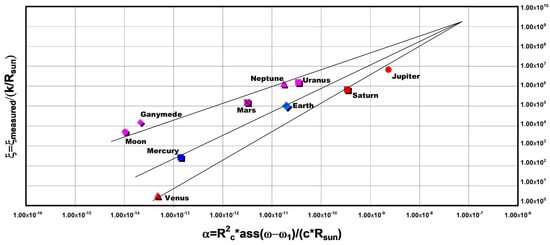
Figure 4.
Parameters for the planets of the solar system.
Looking at this graph, we can assume that the various planets and satellites can be grouped according to the line, characterized by its own single parameter (η) value, on which they lie. This parameter must be a function of the magnetic characteristics of the planet.
Let us express:
where are four dimensionless constants to be found by interpolating the planetary data.
For the parameter η we assume the following definition [2]:
(see [2] for the definition of all quantities). At this point, the magnetic field is known to have up to four constants ki, which can be calculated by imposing the proper value of the magnetic field for each planet or satellite.
Choosing Earth, Jupiter, Venus and the Moon, we obtain the values collected in the following Table 1.

Table 1.
ki values.
Being a function of two parameters, the multiplication factor can be represented geometrically as a surface (Figure 5): this computed amplification surface highlights how different dynamo regimes emerge based on planetary parameters.
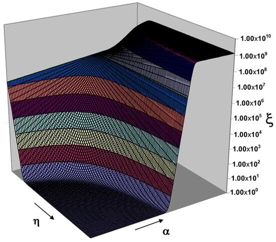
Figure 5.
The multiplicating factor as a surface depending on α, η. The different colors represent the gradual passage from 10i to 10i+1.
7. Summary of the Results and Speculative Remarks
In summary, for a planet we have
From (10), we can deduce that the magnetic field in the solar system—and in the universe more generally—consists of two parts:
- (1)
- The field given by (2), which derives from fundamental principles and is independent of the physical characteristics of the planet;
- (2)
- The amplification factor ξ, given by (4), (8), (9) and Table 1, most likely due to the dynamo effect. The present work does not explain the reason for the previously identified form of this parameter, as such an explanation would require a theoretical study of the dynamo effect).
Evaluating the parameter η for various planets and satellites is challenging. Based on the values from [2], the estimated values are provided in Table 2.
Table 2.
Values of the parameters η and ξ for various planets and satellites (η is taken from [2]) along with the calculated and effective planetary magnetic fields.
As shown by Hcalc/H in Table 2, we find that the model reproduces observed magnetic fields within a reasonable factor, with 0.1 ≤ Hcalc/H ≤ 4.1. Of course, for calibration bodies (Earth, Venus, Jupiter and Moon) the model is exact by construction. For other bodies (e.g., Mars, Mercury, Ganymede), the predictions are within acceptable deviation.
Although important, we intend to notice that there are limitations of the proposed mechanism during the early universe. This SMF generation is unlikely to apply during initial gravitational collapse and instead becomes relevant later when non-synchronous orbital systems emerge.
We present here also two final suggestive remarks related to Equation (2) (in its non-simplified form).
The first is that, from this equation, it can be deduced that in the case of a black hole (BH), any rotating masses in the vicinity of the BH itself would be affected by a field that can assume very significant values. For example, portions of a possible accretion disk gravitating at towards a BH with a mass 3 times that of the Sun would be affected, in the case of non-synchronous rotation, by a field equal to approximately times that of the Earth; this field could explain the phenomenon of the growth of the BH through the loss of angular momentum of the disk itself due to the friction generated by the intense magnetic field (e.g., [33,34]).
The second remark concerns the introduction of a new fractional magnetic source, a sort of ‘metapole’, which, in pairs, forms monopoles [35], but also exhibits some degree of spatial localization, with an 1/r decay in the far magnetic field. Further details can be found in that article.
8. Conclusions
Our study concludes that magnetic fields in celestial bodies might arise from a combination of (i) a universal SMF, generated by the differential orbit and rotational motion of a body orbiting a central mass and (ii) an amplification factor, most likely due to internal dynamo action, which enhances the SMF to the levels observed in planetary and galactic systems. The results show good agreement between the theoretical predictions and observational data, in particular when using galactic magnetic field data [22] and planetary and satellite magnetic field data [2].
While our work does not provide a detailed theoretical explanation for the specific form of the dynamo amplification factor, a more in-depth theoretical investigation of the dynamo effect is needed to fully justify the derived relationships. Nevertheless, our model successfully accounts for magnetic field generation in various astrophysical systems, especially when non-synchronous orbital systems emerge, while presenting some limitations during the early universe, when this SMF generation is unlikely to apply during initial gravitational collapse. The proposed framework is consistent with observational data on both solar system and galactic scales, offering new insights into the role of magnetic fields in astrophysical processes, including potential implications for BH environments, where intense non-synchronous dynamics are present.
Author Contributions
Conceptualization, methodology, investigation A.D.S. and R.D.; writing—original draft preparation, A.D.S. and R.D.; writing—review and editing, A.D.S., R.D. and G.C.; visualization, A.D.S. and G.C. All authors have read and agreed to the published version of the manuscript (R.D. read and agreed to a version that was very close to that submitted).
Funding
This research received some external funding from Ministry of University and Research (MUR) for Unitary project and from Italian Space Agency (ASI) and MUR for Space it Up Project.
Data Availability Statement
The original contributions presented in this study are included in the article. Further inquiries can be directed to the corresponding author.
Conflicts of Interest
The authors declare no conflicts of interest.
Dedication (wrote by A.D.S.)
This work began in 2007 when, out of the blue, Roberto Dini wrote to me, sharing his ingenious ideas about a possible mechanism for generating the seed of all galactic and planetary magnetic fields. Intrigued by his insight, we embarked on an intensive exchange of ideas via email, despite never meeting in person. From that time to about 2010, we then prepared two papers (the first paper has been just published as [11] on Foundations). However, as both of us were deeply engaged in other professional and personal commitments, our collaboration was set aside and remained unfinished for years. Only recently, when I found myself with more time (involving also my collaborator and friend G.C.), I felt compelled to revisit and complete our work. I reached out to Roberto via email, only to receive a notice that the recipient was unknown. A quick search online led me to the heartbreaking discovery that Roberto had passed away in 2020, suffering a fatal heart attack during a video meeting with his colleagues. Though I never had the chance to meet him in person, I came to appreciate, through our many exchanges, his profound understanding of physics and his expertise across multiple scientific disciplines. More than that, I admired his open-mindedness, integrity, and intellectual honesty. This work is, in part, a tribute to his brilliance and passion for discovery.
Appendix A. Definitions
2 GM/c2 gravitational (Schwarzschild) radius of the Sun (or, in general, of the central mass)
generic point-Sun distance (or, in general, generic point – central mass distance)
α2 = 1 − rg/r (square of the) redshift lapse factor
distance center of planet to center of Sun (or of the central mass)
r1 = planet radius
ρ = planet density
angular velocity component around the Sun along the planet’s rotation axis
angular velocity rotation of the planet
magnetic field component along the axis orthogonal to the orbital plane
BH = Black hole
SMF = Seed magnetic field
Appendix B. Derivation of Equation (1) from Fundamental Principles
To derive Equation (1) from first principles (relativity, thermodynamics and electromagnetism), we can follow a speculative but physically motivated pathway. Here is a plausible derivation.
We consider a celestial body in magnetohydrostatic equilibrium, meaning the sum of pressure, gravitational, centrifugal, and magnetic forces vanishes. The body orbits a central mass M with angular velocity ω and rotates on its axis with ω1, where ω ≠ ω1 (non-synchronous rotation). A magnetic field H(r) is assumed to be aligned with the rotation axis (i.e., H//ω1) and radially varying only, so the equation becomes simply scalar.
Key ingredients:
- Weak gravitational Field: Use the Schwarzschild metric in the weak-field limit (.), where rg = 2 GM/c2, is the gravitational radius.
- Electromagnetic Field Energy: The energy density of the magnetic field H in vacuum is .
- Thermodynamic Equilibrium: The system is in equilibrium, so the total energy, including gravitational and electromagnetic contributions, is conserved or extremized (i.e., its time derivative is zero).
- Differential rotation: The celestial body rotates with angular velocity , leading to a relative rotation .
Derivation steps:
Step 1: Conserved quantity in weak gravity
Here we use the conserved Killing/Hamiltonian energy associated with the Schwarzschild time like Killing vector; this is the relevant energy as seen by a distant observer (e.g., [36]). In the weak-field limit, and considering the purely spatial 3-d metric, the effective potential for this electromagnetic field energy density in a curved spacetime can be written as:
where is the metric determinant in Schwarzschild coordinates (for ) and is the correction factor for space-time curvature. The expression (A1) is the “redshifted” energy density as seen at infinity.
Step 2: Equilibrium condition
Assume the system seeks to minimize or conserve the total electromagnetic energy integrated over space. This leads to a conserved quantity, which is the right side of (A1):
This quantity is essentially the locally measured field energy density “redshifted” to infinity, times an area factor. That is why it yields a conserved-like scaling law.
Taking the derivative with respect to r of the expression (A2):
Step 3: Incorporate Differential Rotation
The relative rotation drives the magnetic field configuration. Multiply the equilibrium condition by to account for this:
Divide through H by r2:
This is Equation (1).
Physical Interpretation
- -
- The term Hr2 (1 − rg/r) represents the electromagnetic energy density adjusted for spacetime curvature.
- -
- The equilibrium condition dQ/dr = 0 ensures energy conservation or extremization.
- -
- The factor ω − ω1 encodes the effect of differential rotation on the magnetic field configuration.
Limitations
This derivation is speculative and simplified. A rigorous derivation would require:
- Explicitly solving Maxwell’s equation in curved space-time.
- Including stress-energy tensor contributions from the magnetic field.
- Properly accounting for the thermodynamic equilibrium conditions.
However, the above steps provide a plausible pathway to Equation (1) from first principles.
Appendix C. Checking if Equation (2) Is a Solution of Equation (1)
Given:
- -
- Equation (1):
- -
- Equation (2) (proposed solution):where the approximation is valid when r >> rg.Let us consider the following assumptions:
- -
- , so the term in curly braces must be zero:
As first step, let us compute dH/dr for :
Now, as second step, let us substitute H and dH/dr into the differential equation:
Simplify the first term:
The proposed solution satisfies Equation (1) exactly. The approximation is valid when .
References
- Giovannini, M. The Magnetized Universe. Int. J. Mod. Phys. D 2004, 13, 391–502. [Google Scholar] [CrossRef]
- Olson, P.; Christensen, U.R. Dipole moment scaling for convection-driven planetary dynamos. Earth Planet. Sci. Lett. 2006, 250, 561–571. [Google Scholar] [CrossRef]
- Ichiki, K.; Takahashi, K.; Ohno, H.; Hanayama, H.; Sugiyama, N. Cosmological Magnetic Field: A Fossil of Density Perturbations in the Early Universe. Science 2006, 311, 827–829. [Google Scholar] [CrossRef] [PubMed]
- Han, J.-L. Observing interstellar and intergalactic magnetic fields. Annu. Rev. Astron. Astrophys. 2017, 55, 111–157. [Google Scholar] [CrossRef]
- Brandenburg, A.; Ntormousi, E. Galactic Dynamos. Annu. Rev. Astron. Astrophys. 2023, 61, 561–606. [Google Scholar] [CrossRef]
- Stanley, S. Planetary Dynamos: Updates and New Frontiers. In Heliophysics: Active Stars, Their Astrospheres, and Impacts on Planetary Environments; Cambridge University Press: Cambridge, UK, 2018; Available online: https://lasp.colorado.edu/mop/files/2018/08/Chapter-6.pdf (accessed on 1 May 2025).
- Widrow, L.M. Origin of Galactic and Extragalactic Magnetic Fields. Rev. Mod. Phys. 2002, 74, 775–823. [Google Scholar] [CrossRef]
- Kandus, A.; Kunze, K.E.; Tsagas, C.G. Primordial magnetogenesis. Phys. Rep. 2011, 505, 1–58. [Google Scholar] [CrossRef]
- Subramanian, K. The origin, evolution and signatures of primordial magnetic fields. Rep. Prog. Phys. 2016, 79, 076901. [Google Scholar] [CrossRef]
- Subramanian, K. From Primordial Seed Magnetic Fields to the Galactic Dynamo. Galaxies 2019, 7, 47. [Google Scholar] [CrossRef]
- Martin-Alvarez, S.; Katz, H.; Sijacki, D.; Devriendt, J.; Slyz, A. Unravelling the origin of magnetic fields in galaxies. Mon. Not. R. Astron. Soc. 2021, 504, 2517–2534. [Google Scholar] [CrossRef]
- Turner, M.S.; Widrow, L.M. Inflation-produced, large-scale magnetic fields. Phys. Rev. D 1988, 37, 2743. [Google Scholar] [CrossRef]
- Zweibel, E.G. The Seeds of a Magnetic Universe. Physics 2013, 6, 85. [Google Scholar] [CrossRef]
- Li, S.L. The high-efficiency jets magnetically accelerated from a thin disk in powerful lobe-dominated FRII radio galaxies. Astrophys. J. 2014, 788, 71. [Google Scholar] [CrossRef]
- Crawford, D.A.; Schultz, P.H. Electromagnetic properties of impact-generated plasma, vapor and debris. Int. J. Impact Eng. 1999, 23, 169–180. [Google Scholar] [CrossRef]
- Monteux, J.; Arkani-Hamed, J. Consequences of giant impacts in early Mars: Core merging and Martian dynamo evolution. J. Geophys. Res. Planets 2014, 119, 480–505. [Google Scholar] [CrossRef]
- Buffet, B.A.; Seagle, C.T. Stratification of the top of the core due to chemical interactions with the mantle. J. Geophys. Res. Solid Earth 2010, 115, B4. [Google Scholar] [CrossRef]
- Stevenson, D.J. Planetary magnetic fields. Rep. Prog. Phys. 1983, 46, 555. [Google Scholar] [CrossRef]
- Stevenson, D.J. Planetary magnetic fields. Earth Planet. Sci. Lett. 2003, 208, 1–11. [Google Scholar]
- Russell, C.T. Magnetic fields of the terrestrial planets. J. Geophys. Res. Planets 1993, 98, 18681–18695. [Google Scholar] [CrossRef]
- Beck, R.; Wielebinski, R. Magnetic fields in the Milky Way and in Galaxies. In Planets, Stars and Stellar Systems; Gilmore, G., Ed.; Springer: Berlin/Heidelberg, Germany, 2013; Volume 5, Chapter 13. [Google Scholar]
- Beck, R.; Brandenburg, A.; Moss, D.; Shukurov Sokoloff, D. Galactic Magnetism: Recent developments and perspectives. Annu. Rev. Astron. Astrophys. 1996, 34, 155–206. [Google Scholar] [CrossRef]
- Lyubarsky, Y.E. Transformation of the Poynting flux into kinetic energy in relativistic jets. Mon. Not. R. Astron. Soc. 2010, 402, 353–361. [Google Scholar] [CrossRef]
- Beck, R. Magnetic Fields in Galaxies. Space Sci. Rev. 2012, 166, 215–230. [Google Scholar] [CrossRef]
- Han, J.-L.; Wielebinski, R. Milestones in the Observations of Cosmic Magnetic Fields. Chin. J. Astron. Astrophys. 2002, 2, 293. [Google Scholar] [CrossRef]
- Beck, R. Magnetic fields in spiral galaxies. Astron. Astrophys. Rev. 2016, 24, 4. [Google Scholar] [CrossRef]
- Blackett, P.M.S. The magnetic field of massive rotating bodies. Nature 1947, 159, 658. [Google Scholar] [CrossRef]
- Blackett, P.M.S. A Negative Experiment Relating to Magnetism and the Earth’s Rotation. Philos. Trans. R. Soc. London. Ser. A Math. Phys. Sci. 1952, 245, 309–370. [Google Scholar]
- Kogut, J.B. Special Relativity, Electrodynamics, and General Relativity, 2nd ed.; Academic Press: Cambridge, MA, USA, 2018. [Google Scholar]
- Jacobs, J.A. Planetary magnetic fields. Geophys. Res. Lett. 1979, 6, 213–214, Erratum in Geophys. Res. Lett. 1979, 6, 632. [Google Scholar]
- Dolginov, S.S. The magnetic field and the magnetosphere of the planet Mars. Adv. Space Res. 1992, 12, 187–211. [Google Scholar] [CrossRef]
- Chiappini, M.; De Santis, A. Magnetic investigations for studying planetary interiors. Ann. Geophys. 1994, 37, 1–14. [Google Scholar] [CrossRef]
- Blandford, R.D.; Znajek, R.L. Electromagnetic extraction of energy from Kerr black holes. Mon. Not. R. Astron. Soc. 1977, 179, 433–456. [Google Scholar] [CrossRef]
- Balbus, S.A.; Hawley, J.F. A powerful local shear instability in weakly magnetized disks. I—Linear analysis. II—Nonlinear evolution. Astrophys. J. 1991, 376, 214–233. [Google Scholar] [CrossRef]
- De Santis, A.; Dini, R. Beyond Classical Multipoles: The Magnetic Metapole as an Extended Field Source. Foundations 2025, 5, 25. [Google Scholar] [CrossRef]
- Wald, R.M. General Relativity; The University of Chicago Press: Chicago, IL, USA, 1984; p. 491. [Google Scholar]
Disclaimer/Publisher’s Note: The statements, opinions and data contained in all publications are solely those of the individual author(s) and contributor(s) and not of MDPI and/or the editor(s). MDPI and/or the editor(s) disclaim responsibility for any injury to people or property resulting from any ideas, methods, instructions or products referred to in the content. |
© 2025 by the authors. Licensee MDPI, Basel, Switzerland. This article is an open access article distributed under the terms and conditions of the Creative Commons Attribution (CC BY) license (https://creativecommons.org/licenses/by/4.0/).