Galerkin Finite Element Approximation of a Stochastic Semilinear Fractional Wave Equation Driven by Fractionally Integrated Additive Noise

Abstract

We investigate the application of the Galerkin finite element method to approximate a stochastic semilinear space–time fractional wave equation. The equation is driven by integrated additive noise, and the time fractional order $\alpha \in (1,2)$. The existence of a unique solution of the problem is proved by using the Banach fixed point theorem, and the spatial and temporal regularities of the solution are established. The noise is approximated with the piecewise constant function in time in order to obtain a stochastic regularized semilinear space–time wave equation which is then approximated using the Galerkin finite element method. The optimal error estimates are proved based on the various smoothing properties of the Mittag–Leffler functions. Numerical examples are provided to demonstrate the consistency between the theoretical findings and the obtained numerical results.

1. Introduction

Consider the following stochastic semilinear space–time fractional wave equation driven by fractionally integrated additive noise, with $1<\alpha <2,$ $\frac{1}{2}<\beta \le 1,$ $0\le \gamma \le 1,$

$$\begin{array}{cc}\hfill & {}_0^C{D}_t^{\alpha }u(t,x)+{(-\Delta )}^{\beta }u(t,x)=f(t,u(t,x))+{}_0^R{D}_t^{-\gamma }\frac{{\partial }^{2}W(t,x)}{\partial t\partial x},0<t<T,x\in D,\hfill \\ \hfill & u(t,x)=0,0<t<T,x\in \partial D,\hfill \\ \hfill & u(0,x)=v_1\left(x\right),\frac{\partial u(0,x)}{\partial t}=v_2\left(x\right),x\in D,\hfill \end{array}$$

(1)

where D is a bounded domain in ${\mathbb{R}}^d,$ $d=1,2,3$ with smooth boundary $\partial D$, and ${}_0^C{D}_t^{\alpha }u\left(t\right)$ and ${}_0^R{D}_t^{-\gamma }u\left(t\right)$ represent the Caputo fractional derivative of order $\alpha \in (1,2)$ and the Riemann–Liouville fractional integral of order $\gamma \in [0,1],$ respectively. In addition, ${(-\Delta )}^{\beta }$ is the fractional Laplacian and $\frac{{\partial }^{2}W(t,x)}{\partial t\partial x}$ denotes the space–time noise defined on a complete filtered probability space $\left(\mathsf{\Omega },\mathcal{F},{\left\{{\mathcal{F}}_t\right\}}_{t\ge 0},\mathbb{P}\right).$ The initial values $v_1$ and $v_2$ and the nonlinear function (source term) $f(t,y),y\in \mathbb{R}$ are given functions.

The space–time fractional wave equation, denoted as (1) when devoid of noise, has been extensively explored by researchers due to its wide range of applications in engineering, physics, and biology [1,2,3]. The inclusion of the noise term $\frac{{\partial }^{2}W(t,x)}{\partial t\partial x}$ allows for the characterization of random effects influencing the particle movement within a medium with memory or particles experiencing sticking and trapping phenomena. An example of such noise is the fractionally integrated noise ${}_0^R{D}_t^{-\gamma }\frac{{\partial }^{2}W(t,x)}{\partial t\partial x}$, where the past random effects impact the internal energy [4]. For physical systems, stochastic perturbations arise from many natural sources, which cannot always be ignored. Therefore, it is necessary to include them in the corresponding deterministic model.

It is not possible to find the analytic solution of the space–time fractional Equation (1). Therefore, one needs to introduce and analyze some efficient numerical methods for solving (1). Li et al. [5] considered the Galerkin finite element method of (1) for the linear case with the additive Gaussian noise, that is, $f=0$ and $\gamma =0$, and obtain the error estimates. In [6], the authors studied the Galerkin finite element method for approximating the semilinear stochastic time-tempered fractional wave equations with multiplicative Gaussian noise and additive fractional Gaussian noise, but they only established error estimates for $\alpha \in (\frac{3}{2},2)$. Extensive theoretical results exist for the stochastic subdiffusion problem with $\alpha \in (0,1)$, as seen in works such as [7,8,9,10,11,12], alongside corresponding numerical approximations in works including [13,14,15,16,17]. Regarding the theoretical and numerical findings for the stochastic wave equation, we recommend exploring references such as [18,19,20,21]. For theoretical advancements in fractional-order nonlinear differential equations, recent works such as [22,23,24,25,26,27] and their references provide a comprehensive overview.

In this paper, our focus lies on the application of the Galerkin finite element method to solve (1). Firstly, we establish the existence of a unique solution for (1) using the Banach fixed point theorem. Additionally, we analyze the spatial and temporal regularities of the solution. To approximate the noise, we employ a piecewise constant function in time, resulting in a stochastic regularized equation. This equation is then tackled using the Galerkin finite element method. We provide corresponding error estimates, utilizing the various smoothing properties exhibited by the Mittag–Leffler functions. We extend the error estimates in [5] from the linear case of (1) with Gaussian additive noise to the semilinear case with the more general integrated additive noise. We also extend the error estimates of [6] for the stochastic semilinear time fractional wave equation from $\alpha \in (\frac{3}{2},2)$ to $\alpha \in (1,2)$.

To establish our error estimates, we employ a similar argument as developed in our recent work [28], which focused on approximating the stochastic semilinear subdiffusion equation with $\alpha \in (0,1)$. We demonstrate that the solution’s spatial and temporal regularities for (1) with $\alpha \in (1,2)$ surpass those with $\alpha \in (0,1)$. Moreover, we observe that the convergence orders of the Galerkin finite element method for (1) with $\alpha \in (1,2)$ are higher than those with $\alpha \in (0,1)$, as expected.

The paper is organized as follows. In Section 2, we provide some preliminaries and notations. In Section 3, we focus on the continuous problem and establish the existence, uniqueness, and regularity results for the problem (1). In Section 4, we discuss the approximation of the noise and obtain an error estimate for the regularized stochastic semilinear fractional superdiffusion problem. In Section 5, we consider the finite element approximation of the regularized problem and derive optimal error estimates. Finally, in Section 6, we present numerical experiments that validate our theoretical findings.

Throughout this paper, we denote C as a generic constant that is independent of the step size $\tau$ and the space step size h, which could be different at different occurrences. Additionally, we always assume $ϵ>0$ is a small positive constant.

2. Notation and Preliminaries

This section provides notations and preliminary results that will be used in subsequent sections. We denote $H=L^2\left(D\right)$ as the space of Lebesgue measurable or square integrable functions on D, with norm $|·|$ and inner product $(·,·)$. Additionally, we denote $H_0^1=\{vs.\in H^1:vs.=0\mathrm{on}\partial D\}$. We assume that $A=-\Delta$ with domain $D\left(A\right)=H^2\left(D\right)\cap H_0^1\left(D\right)$ is a closed linear self-adjoint positive definite operator with a compact inverse. Moreover, A has the eigenpairs $({\lambda }_k,{\varphi }_k)$, $k=1,2,3,\cdots$, subject to homogeneous Dirichlet boundary conditions.

Set ${\dot{H}}^s\left(D\right)$ or simply ${\dot{H}}^s$ for any $s\in \mathbb{R}$ as a Hilbert space induced by the norm

$$\begin{array}{c}\hfill {|vs.|}_s^2:=\sum _{k=1}^{\infty }{\lambda }_k^s{(v,{\varphi }_k)}^2.\end{array}$$

For $s=0,$ we denote ${\dot{H}}^0$ by $H.$ For any function $\psi \in {\dot{H}}^{2\beta },$ $\frac{1}{2}<\beta \le 1,$ define ${(-\Delta )}^{\beta }\psi :={\sum }_{k=1}^{\infty }{\lambda }_k^{\beta }(\psi ,{\varphi }_k){\varphi }_k.$ Let $L^2(\mathsf{\Omega };{\dot{H}}^s),s\in \mathbb{R}$ be a separable Hilbert space of all measurable square-integrable random variables $\varphi$ with values in ${\dot{H}}^s$ such that ${\parallel \varphi \parallel }_{L^2(\mathsf{\Omega };{\dot{H}}^s)}:={(\mathbf{E}|\varphi |}_s^2{)}^{\frac{1}{2}}<\infty ,$ where $\mathbf{E}$ denotes the expectation.

Define the space–time noise $\frac{{\partial }^{2}W(t,x)}{\partial t\partial x}$ by, see [28],

$$\frac{{\partial }^{2}W(t,x)}{\partial t\partial x}=\sum _{k=1}^{\infty }{\sigma }_k\left(t\right){\dot{\beta }}_k\left(t\right){\varphi }_k\left(x\right),$$

(2)

where ${\sigma }_k(·),k=1,2,3,\cdots ,$ are some real-valued continuous functions rapidly decaying with respect to k. Here, the sequence ${\left\{{\beta }_k\right\}}_{k=1}^{\infty }$ is mutually independent and identically distributed one-dimensional standard Brownian motions, and the white noise ${\dot{\beta }}_k\left(t\right)=\frac{d{\beta }_k\left(t\right)}{dt},k=1,2,3,\cdots ,$ is the formal derivative of the Brownian motion ${\beta }_k\left(t\right).$

Lemma 1

([28]). (It$\tilde{o}$ isometry property) Let $\psi :[0,T]\times \mathsf{\Omega }\to H$ be a strongly measurable mapping such that ${\int }_0^t\mathbf{E}{\parallel \psi \left(s\right)\parallel }^{2}ds<\infty .$ Let $B\left(t\right)$ denote a real-valued standard Brownian motion. Then, the following isometry equality holds for $t\in (0,T]$:

$$\mathbf{E}\parallel {\int }_0^t{\psi \left(s\right)dB\left(s\right)\parallel }^2={\int }_0^t\mathbf{E}{\parallel \psi \left(s\right)\parallel }^{2}ds.$$

(3)

To represent the solution of (1) in the integral form, we utilize the Laplace transform technique to write down the solution representation in terms of the Mittag–Leffler functions. The Mittag–Leffler functions are defined in [28], and we use them to express the solution in a compact form.

$$E_{\overline{\alpha },\overline{\beta }}\left(z\right)=\sum _{k=0}^{\infty }\frac{z^k}{\mathsf{\Gamma }\mathsf{(}k\overline{\alpha }+\overline{\beta })},\mathrm{for}z\in \mathbb{C},\overline{\alpha }>0,\overline{\beta }\in \mathbb{R}.$$

(4)

The following Lemma is related to the bounds of the Mittag–Leffler functions.

Lemma 2

((Mittag–Leffler function property) [28]). Let $1<\overline{\alpha }<2$ and $\overline{\beta }\in \mathbb{R}$. Let $E_{\overline{\alpha },\overline{\beta }}$ be defined by (4). Suppose that μ is an arbitrary real number such that $\frac{\pi \overline{\alpha }}{2}<\mu <min(\pi ,\pi \overline{\alpha })=\pi .$ Then, there exists a constant $C=C(\overline{\alpha },\overline{\beta },\mu )>0$ such that

$$|E_{\overline{\alpha },\overline{\beta }}\left(z\right)|\le \frac{C}{1+\left|z\right|},\mu \le |arg\left(z\right)|\le \pi .$$

(5)

Moreover, for $\lambda >0,\overline{\alpha }>0,\overline{\beta }>0,\overline{\gamma }>0,\overline{\gamma }\ne 1,$ it follows that

$$\frac{d}{dt}\left(t^{\overline{\gamma }-1}{E}_{\overline{\alpha },\overline{\gamma }}(-{\lambda }^{\overline{\beta }}{t}^{\overline{\alpha }})\right)=t^{\overline{\gamma }-2}{E}_{\overline{\alpha },\overline{\gamma }-1}(-{\lambda }^{\overline{\beta }}{t}^{\overline{\alpha }}),t>0.$$

(6)

3. Existence, Uniqueness, and Regularity Results

This section is dedicated to studying the existence, uniqueness, and regularity results of the mild solution of the stochastic semilinear space–time fractional superdiffusion model (1).

Assumption 1.

There is a positive constant C such that the nonlinear function $f:{\mathbb{R}}^{+}\times H\to H$ satisfies

$$\parallel f(t_1,u_1)-f(t_2,u_2)\parallel \le C\left(|t_1-t_2|+\parallel u_1-u_2\parallel \right),$$

(7)

and

$$\parallel f(t,u)\parallel \le C(1+\parallel u\parallel ).$$

(8)

Assumption 2.

The sequence $\left\{{\sigma }_k\left(t\right)\right\}$ with its derivative is uniformly bounded by ${\mu }_k$ and ${\gamma }_k$, respectively, i.e.,

$$|{\sigma }_k\left(t\right)|\le {\mu }_k,$$

(9)

$$|{\sigma }_k^{\prime }\left(t\right)|\le {\gamma }_k,\forall t\in [0,T],$$

(10)

where the series ${\sum }_{k=1}^{\infty }{\mu }_k$ and ${\sum }_{k=1}^{\infty }{\gamma }_k$ are convergent.

Assumption 3.

Let $1<\alpha <2,\frac{1}{2}<\beta \le 1,0\le \gamma \le 1.$ It holds, with $0\le r\le \kappa ,$

$$\sum _{k=1}^{\infty }{\mu }_k^2{\lambda }_k^{r-\kappa }<\infty ,$$

where

$$\kappa =\left\{\begin{array}{cc}2\beta ,\hfill & \gamma >\frac{1}{2},\hfill \\ (2-\frac{1-2\gamma }{\alpha })\beta -ϵ,\hfill & \gamma \le \frac{1}{2},\hfill \end{array}\right.$$

and ${\lambda }_k,k=1,2,\cdots$ are the eigenvalues of the Laplacian $A=-\Delta ,$ with $D\left(A\right)=H_0^1\left(D\right)\cap H^2\left(D\right).$

Lemma 3

([5], Lemma 2.4). An adapted process ${\left\{u\left(t\right)\right\}}_{t\ge 0}$ is called a mild solution to (1) if it satisfies the following integral equation with $1<\alpha <2,\frac{1}{2}<\beta \le 1,0\le \gamma \le 1,$

$$u(t,x)={\mathbb{E}}_{\alpha ,\beta }\left(t\right)v_1+{\tilde{\mathbb{E}}}_{\alpha ,\beta }\left(t\right)v_2+{\int }_0^t{\overline{\mathbb{E}}}_{\alpha ,\beta }(t-s)f(s,u\left(s\right))ds+{\int }_0^t{\overline{\mathbb{E}}}_{\alpha ,\beta ,\gamma }(t-s)dW\left(s\right),$$

(11)

where $dW\left(s\right)$ denotes

$$dW\left(s\right)=\sum _{k=1}^{\infty }{\sigma }_k\left(s\right){\varphi }_{k}d{\beta }_k\left(s\right),$$

and

$$\begin{array}{cc}\hfill & {\mathbb{E}}_{\alpha ,\beta }\left(t\right)v_1:=\sum _{k=1}^{\infty }{E}_{\alpha ,1}(-{\lambda }_k^{\beta }{t}^{\alpha })(v_1,{\varphi }_k){\varphi }_k,{\tilde{\mathbb{E}}}_{\alpha ,\beta }\left(t\right)v_2:=\sum _{k=1}^{\infty }t{E}_{\alpha ,2}(-{\lambda }_k^{\beta }{t}^{\alpha })(v_2,{\varphi }_k){\varphi }_k,\hfill \\ \hfill & {\overline{\mathbb{E}}}_{\alpha ,\beta }\left(t\right)vs.:=\sum _{k=1}^{\infty }{t}^{\alpha -1}{E}_{\alpha ,\alpha }(-{\lambda }_k^{\beta }{t}^{\alpha })(v,{\varphi }_k){\varphi }_k,{\overline{\mathbb{E}}}_{\alpha ,\beta ,\gamma }\left(t\right)vs.:=\sum _{k=1}^{\infty }{t}^{\alpha +\gamma -1}{E}_{\alpha ,\alpha +\gamma }(-{\lambda }_k^{\beta }{t}^{\alpha })(v,{\varphi }_k){\varphi }_k.\hfill \end{array}$$

Lemma 4

([5], Lemma 2.5). The solution $u\left(t\right)$ of the homogenuous problem of (1) satisfies, for $t>0$,

$$\begin{array}{c}\hfill {\left|u\left(t\right)\right|}_p\le \left\{\begin{array}{c}C{t}^{-\frac{\alpha (p-q)}{2\beta }}|v_1{|}_q+C{t}^{1-\frac{\alpha (p-r)}{2\beta }}{\left|v_2\right|}_r,0\le q,r\le p\le 2\beta ,\hfill \\ C{t}^{-\alpha }|v_1{|}_q+C{t}^{1-\alpha }{\left|v_2\right|}_r,q,r>p,\hfill \end{array}\right.\end{array}$$

(12)

and it also implies that

$$|{\partial }_t^{\alpha }{u\left(t\right)|}_p\le C{t}^{-\alpha -\alpha \frac{p-q}{2\beta }}|v_1{|}_q+C{t}^{-\alpha +1-\alpha \frac{p-r}{2\beta }}{\left|v_2\right|}_r.$$

(13)

Lemma 5

([28]). Let $1<\alpha <2$, $\frac{1}{2}<\beta \le 1$, $0\le \gamma \le 1.$ For any $t>0$ and $0\le p-q\le 2\beta ,$ there holds,

$$|{\overline{\mathbb{E}}}_{\alpha ,\beta ,\gamma }{\left(t\right)v|}_p\le C{t}^{-1+(\alpha +\gamma )-\alpha \frac{(p-q)}{2\beta }}{|vs.|}_q.$$

(14)

Theorem 1

(Existence and uniqueness). Let $1<\alpha <2,$ $\frac{1}{2}<\beta \le 1$ and $0\le \gamma \le 1$. Let Assumptions 1–3 hold. Let $v_1,v_2\in L^2(\mathsf{\Omega };H)$. Then, there exists a unique mild solution $u\in C\left([0,T];L^2(\mathsf{\Omega };H)\right)$ given by (11) to the problem (1) for all $t\in [0,T].$

Proof. 

Set $C{\left([0,T];L^2(\mathsf{\Omega };H)\right)}_{\lambda },$ $\lambda >0$, as the set of functions in $C\left([0,T];L^2(\mathsf{\Omega };H)\right)$ with the following weighted norm ${\parallel u\parallel }_{\lambda }^2:={sup}_{t\in [0,T]}\mathbf{E}\left(\parallel e^{-\lambda t}{u\left(t\right)\parallel }^2\right)$ $\forall u\in C{\left([0,T];L^2(\mathsf{\Omega };H)\right)}_{\lambda }.$ For any fixed $\lambda >0$ this norm is the same as the standard norm on $C\left([0,T];L^2(\mathsf{\Omega };H)\right).$ We can therefore define a nonlinear map $\mathcal{T}:C{\left([0,T];L^2(\mathsf{\Omega };H)\right)}_{\lambda }\to C{\left([0,T];L^2(\mathsf{\Omega };H)\right)}_{\lambda }$ by

$$\mathcal{T}u\left(t\right)={\mathbb{E}}_{\alpha ,\beta }\left(t\right)v_1+{\tilde{\mathbb{E}}}_{\alpha ,\beta }\left(t\right)v_2+{\int }_0^t{\overline{\mathbb{E}}}_{\alpha ,\beta }(t-s)f(s,u\left(s\right))ds+{\int }_0^t{\overline{\mathbb{E}}}_{\alpha ,\beta ,\gamma }(t-s)dW\left(s\right).$$

(15)

For any $\lambda >0,$ the function $u\in C\left([0,T];L^2(\mathsf{\Omega };H)\right)$ is a solution of (11) if and only if u is a fixed point of the map $\mathcal{T}:C{\left([0,T];L^2(\mathsf{\Omega };H)\right)}_{\lambda }\to C{\left([0,T];L^2(\mathsf{\Omega };H)\right)}_{\lambda }$. In order to apply the Banach fixed point theorem it suffices to show that for an appropriately chosen $\lambda >0,\mathcal{T}$ is a contraction mapping. We first show that $\mathcal{T}u\in C\left([0,T];L^2(\mathsf{\Omega };H)\right)$ for any $u\in C\left([0,T];L^2(\mathsf{\Omega };H)\right)$. By (15) and the Cauchy–Schwarz inequality we obtain with $u\in C\left([0,T];L^2(\mathsf{\Omega };H)\right),$

$$\begin{array}{cc}\hfill {\mathbf{E}\parallel \mathcal{T}u\left(t\right)\parallel }^2& \le 4\mathbf{E}\parallel {\mathbb{E}}_{\alpha ,\beta }\left(t\right)v_1{\parallel }^2+4\mathbf{E}\parallel {\tilde{\mathbb{E}}}_{\alpha ,\beta }\left(t\right)v_2{\parallel }^2+4\mathbf{E}{\parallel {\int }_0^t{\overline{\mathbb{E}}}_{\alpha ,\beta }(t-s)f(s,u\left(s\right))ds\parallel }^2\hfill \\ \hfill & +4\mathbf{E}\parallel {\int }_0^t{\overline{\mathbb{E}}}_{\alpha ,\beta ,\gamma }{(t-s)dW\left(s\right)\parallel }^2\hfill \\ \hfill & \le 4\mathbf{E}\parallel {\mathbb{E}}_{\alpha ,\beta }\left(t\right)v_1{\parallel }^2+4\mathbf{E}\parallel {\tilde{\mathbb{E}}}_{\alpha ,\beta }\left(t\right)v_2{\parallel }^2+4t{\int }_0^t\mathbf{E}{\parallel {\overline{\mathbb{E}}}_{\alpha ,\beta }(t-s)f(s,u\left(s\right))\parallel }^{2}ds\hfill \\ \hfill & +4\mathbf{E}\parallel {\int }_0^t{\overline{\mathbb{E}}}_{\alpha ,\beta ,\gamma }{(t-s)dW\left(s\right)\parallel }^2.\hfill \end{array}$$

Based on the smoothing properties of the solution operators and by Assumption 1, it follows that

$$\begin{array}{cc}\hfill {\mathbf{E}\parallel \mathcal{T}u\left(t\right)\parallel }^2& \le C\mathbf{E}\parallel v_1{\parallel }^2+C\mathbf{E}{\parallel v_2\parallel }^2+Ct{\int }_0^t{(t-s)}^{2(-1+\alpha )}\left(1+{\mathbf{E}\parallel u\left(s\right)\parallel }^2\right)ds\hfill \\ \hfill & +C\mathbf{E}\parallel {\int }_0^t{\overline{\mathbb{E}}}_{\alpha ,\beta ,\gamma }{(t-s)dW\left(s\right)\parallel }^2.\hfill \end{array}$$

(16)

By the smoothing property of the operator ${\overline{\mathbb{E}}}_{\alpha ,\beta ,\gamma },$ the isometry property of Brownian motion, we have with $0\le r\le \kappa$ that,

$$\begin{array}{cc}\hfill & \mathbf{E}\parallel {\int }_0^t{\overline{\mathbb{E}}}_{\alpha ,\beta ,\gamma }{(t-s)dW\left(s\right)\parallel }^2=\mathbf{E}{\parallel {\int }_0^t{A}^{\frac{\kappa -r}{2}}{\overline{\mathbb{E}}}_{\alpha ,\beta ,\gamma }(t-s)\sum _{k=1}^{\infty }{\sigma }_k\left(s\right)A^{\frac{r-\kappa }{2}}{\varphi }_{k}d{\beta }_k\left(s\right)\parallel }^2\hfill \\ \hfill & =\sum _{k=1}^{\infty }{\int }_0^t{\parallel A^{\frac{\kappa -r}{2}}{\overline{\mathbb{E}}}_{\alpha ,\beta ,\gamma }(t-s){\sigma }_k\left(s\right)A^{\frac{r-\kappa }{2}}{\varphi }_k\parallel }^{2}ds\le C\left({\int }_0^t{\parallel A^{\frac{\kappa -r}{2}}{\overline{\mathbb{E}}}_{\alpha ,\beta ,\gamma }\left(s\right)\parallel }^{2}ds\right)\left(\sum _{k=1}^{\infty }{\mu }_k^2{\lambda }_k^{r-\kappa }\right)\hfill \\ \hfill & \le C\left(\sum _{k=1}^{\infty }{\mu }_k^2{\lambda }_k^{r-\kappa }\right){\int }_0^t{\left(s^{\alpha +\gamma -1-\frac{\kappa -r}{2\beta }\alpha }\right)}^{2}ds\le C\left(\sum _{k=1}^{\infty }{\mu }_k^2{\lambda }_k^{r-\kappa }\right){\int }_0^t{s}^{\alpha (2-\frac{\kappa -r}{\beta })+2\gamma -2}ds\hfill \\ \hfill & \le C\left(\sum _{k=1}^{\infty }{\mu }_k^2{\lambda }_k^{r-\kappa }\right)<\infty .\hfill \end{array}$$

(17)

Note that $v_1,v_2\in L^2(\mathsf{\Omega };H)$ and $u\in C\left([0,T];L^2(\mathsf{\Omega };H)\right)$; we then obtain ${sup}_{t\in [0,T]}\mathbf{E}{\parallel \mathcal{T}u\parallel }^2<\infty$, which implies that $\mathcal{T}u\in C\left([0,T];L^2(\mathsf{\Omega };H)\right)$. Now we consider the contraction property. For any given two functions $u_1$ and $u_2$ in $C{\left([0,T];L^2(\mathsf{\Omega };H)\right)}_{\lambda },$ it follows from (15) with the smoothing property and boundedness of ${\overline{\mathbb{E}}}_{\alpha ,\beta ,\gamma }$ with $p=0$ and $q=0$ that

$$\begin{array}{cc}\hfill \mathbf{E}\parallel e^{-\lambda t}(\mathcal{T}{u}_1-\mathcal{T}{u}_2)\left(t\right){\parallel }^2& =\mathbf{E}\parallel e^{-\lambda t}{\int }_0^t{\overline{\mathbb{E}}}_{\alpha ,\beta }(t-s)\left(f\left(u_1\left(s\right)\right)-f\left(u_2\left(s\right)\right)\right)ds{\parallel }^2\hfill \\ \hfill & =\mathbf{E}\parallel {\int }_0^{t}1·\left[e^{-\lambda (t-s)}{\overline{\mathbb{E}}}_{\alpha ,\beta }(t-s)\right]\left[e^{-\lambda s}\left(f\left(u_1\left(s\right)\right)-f\left(u_2\left(s\right)\right)\right)\right]ds{\parallel }^2\hfill \\ \hfill & \le Ct\mathbf{E}{\int }_0^t\parallel \left[e^{-\lambda (t-s)}{\overline{\mathbb{E}}}_{\alpha ,\beta }(t-s)\right]\left[e^{-\lambda s}\left(f\left(u_1\left(s\right)\right)-f\left(u_2\left(s\right)\right)\right)\right]{\parallel }^{2}ds\hfill \\ \hfill & \le Ct\left[{\int }_0^t{\parallel e^{-\lambda (t-s)}{\overline{\mathbb{E}}}_{\alpha ,\beta }(t-s)\parallel }^{2}ds\right]·{\parallel u_1-u_2\parallel }_{\lambda }^2.\hfill \end{array}$$

Note that

$$\begin{array}{cc}\hfill & t{\int }_0^t{\parallel e^{-\lambda (t-s)}{\overline{\mathbb{E}}}_{\alpha ,\beta }(t-s)\parallel }^{2}ds\le Ct{\int }_0^t{e}^{-2\lambda (t-s)}{(t-s)}^{2(\alpha -1)}ds\hfill \\ \hfill & =Ct{\int }_0^t{e}^{-2\lambda \tau }{\tau }^{2(\alpha -1)}d\tau =Ct\left[{\int }_0^t{e}^{-2x}{x}^{2\alpha -2}dx\right]{\lambda }^{1-2\alpha }\le Ct\left[{\int }_0^{\infty }{e}^{-2x}{x}^{2\alpha -2}dx\right]{\lambda }^{1-2\alpha }\le C\left(T\right){\lambda }^{1-2\alpha }.\hfill \end{array}$$

With $\alpha \in (1,2)$, choose sufficiently large $\lambda$, we obtain

$$\begin{array}{c}\hfill \mathbf{E}\parallel e^{-\lambda t}(\mathcal{T}{u}_1-\mathcal{T}{u}_2)\left(t\right){\parallel }^2\le C\left(T\right){\lambda }^{1-2\alpha }\parallel u_1-u_2{\parallel }_{\lambda }^2\le \delta {\parallel u_1-u_2\parallel }_{\lambda }^2,\mathrm{for} \mathrm{some}0<\delta <1.\end{array}$$

Hence, $\parallel \mathcal{T}\left(u_1\right)-\mathcal{T}\left(u_2\right){\parallel }_{\lambda }\le \delta {\parallel u_1-u_2\parallel }_{\lambda }.$ Therefore, by the Banach contraction mapping theorem, there exists a unique fixed point u of the nonlinear map $\mathcal{T}$ which is the mild solution given by (15) of the problem (1).    □

Theorem 2.

(Regularity) Let $1<\alpha <2,\frac{1}{2}<\beta \le 1,0\le \gamma \le 1.$ Assume that Assumptions 1–3 hold. Let $v_1\in L^2(\mathsf{\Omega };{\dot{H}}^q)$, $v_2\in L^2(\mathsf{\Omega };{\dot{H}}^p)$ with $p,q\in [0,2\beta ].$ Then, the following regularity results hold for the solution u of (11) with $r\in [0,\kappa ]$ and $0\le p\le r\le 2\beta ,0\le q\le r\le 2\beta$,

$$\begin{array}{c}\hfill {\mathbf{E}\left|u\left(t\right)\right|}_r^2\le C{t}^{\alpha \frac{(q-r)}{\beta }}|v_1{|}_q^2+C{t}^{2-\alpha \frac{(r-p)}{\beta }}{|v_2|}_p^2+C\mathbf{E}\left(\underset{s\in [0,T]}{sup}{\parallel u\left(s\right)\parallel }^2\right)+C\left(\sum _{k=1}^{\infty }{\mu }_k^2{\lambda }_k^{r-\kappa }\right).\end{array}$$

(18)

Proof. 

From the definition of the mild solution (11) and $t\in (0,T]$ with $0\le p, q\le r\le 2\beta ,$ it follows that, with $r\in [0,\kappa ],$

$$\begin{array}{cc}\hfill {\mathbf{E}|u\left(t\right)|}_r^2\le & 4(\mathbf{E}|{\mathbb{E}}_{\alpha ,\beta }{v}_1{|}_r^2+\mathbf{E}|{\tilde{\mathbb{E}}}_{\alpha ,\beta }\left(t\right)v_2{|}_r^2+\mathbf{E}|{\int }_0^t{\overline{\mathbb{E}}}_{\alpha ,\beta }(t-s)f(s,u\left(s\right))ds{|}_r^2\hfill \\ \hfill & +\mathbf{E}|{\int }_0^t{\overline{\mathbb{E}}}_{\alpha ,\beta ,\gamma }{(t-s)dW\left(s\right)|}_r^2)\le 4\left(I_1+I_2+I_3+I_4\right).\hfill \end{array}$$

(19)

For $I_1$ and $I_2$, by the regularity Lemma in [5], we have

$$I_1=\mathbf{E}|{\mathbb{E}}_{\alpha ,\beta }\left(t\right)v_1{|}_r^2\le C{t}^{\alpha \frac{(q-r)}{\beta }}{|v_1|}_q^2,$$

(20)

and

$$I_2=\mathbf{E}|{\tilde{\mathbb{E}}}_{\alpha ,\beta }{\left(t\right)|}_r^2\le C{t}^{2-\alpha \frac{(r-p)}{\beta }}{|v_2|}_p^2,\mathrm{for}\frac{r-p}{\beta }\le 2.$$

(21)

For $I_3$ using the smoothing property of the operator ${\overline{\mathbb{E}}}_{\alpha ,\beta }\left(t\right)$ and the Assumption 1, we have

$$\begin{array}{cc}\hfill I_3& =\mathbf{E}|{\int }_0^t{\overline{\mathbb{E}}}_{\alpha ,\beta }{(t-s)f(s,u\left(s\right))ds|}_r^2\le \mathbf{E}{\left({\int }_0^t{|{\overline{\mathbb{E}}}_{\alpha ,\beta }(t-s)f(s,u\left(s\right))|}_{r}ds\right)}^2\hfill \\ \hfill & \le C\mathbf{E}{\left({\int }_0^t{(t-s)}^{\alpha -1+\alpha \frac{(r-0)}{\beta }}\parallel f(s,u\left(s\right))\parallel ds\right)}^2\hfill \\ \hfill & \le C{\left({\int }_0^t{(t-s)}^{\alpha -1+\alpha \left(\frac{r-0}{\beta }\right)}ds\right)}^2\mathbf{E}{\left[\underset{s\in [0,T]}{sup}\parallel f(s,u\left(s\right))\parallel \right]}^2\le C\mathbf{E}\left(\underset{s\in [0,T]}{sup}{\parallel u\left(s\right)\parallel }^2\right).\hfill \end{array}$$

(22)

For $I_4$, by isometry property of the Brownian motion and Assumption 2 and the smoothing property of the operator ${\overline{\mathbb{E}}}_{\alpha ,\beta ,\gamma }\left(t\right)$, we arrive at, with $0\le r\le \kappa$,

$$\begin{array}{cc}\hfill I_4& =\mathbf{E}\parallel {\int }_0^t{A}^{\frac{r}{2}}{\overline{\mathbb{E}}}_{\alpha ,\beta ,\gamma }{(t-s)dW\left(s\right)\parallel }^2=\mathbf{E}{\parallel {\int }_0^t{A}^{\frac{\kappa }{2}}{\overline{\mathbb{E}}}_{\alpha ,\beta ,\gamma }(t-s)\sum _{k=1}^{\infty }{\sigma }_k\left(s\right)A^{\frac{r-\kappa }{2}}{\varphi }_{k}d{\beta }_k\left(s\right)\parallel }^2\hfill \\ \hfill & =\sum _{k=1}^{\infty }{\int }_0^t{\parallel A^{\frac{\kappa }{2}}{\overline{\mathbb{E}}}_{\alpha ,\beta ,\gamma }(t-s){\sigma }_k\left(s\right)A^{\frac{r-\kappa }{2}}{\varphi }_k\parallel }^{2}ds\le C\left({\int }_0^t{\parallel A^{\frac{\kappa }{2}}{\overline{\mathbb{E}}}_{\alpha ,\beta ,\gamma }\left(s\right)\parallel }^{2}ds\right)\left(\sum _{k=1}^{\infty }{\mu }_k^2{\lambda }_k^{r-\kappa }\right)\hfill \\ \hfill & \le C\left(\sum _{k=1}^{\infty }{\mu }_k^2{\lambda }_k^{r-\kappa }\right){\int }_0^t{\left(s^{\alpha +\gamma -1-\alpha \frac{(\kappa -0)}{2\beta }}\right)}^{2}ds=C\left(\sum _{k=1}^{\infty }{\mu }_k^2{\lambda }_k^{r-\kappa }\right){\int }_0^t{s}^{\alpha (2-\frac{\kappa }{\beta })+2\gamma -2}ds,\hfill \\ \hfill & \le C\left(\sum _{k=1}^{\infty }{\mu }_k^2{\lambda }_k^{r-\kappa }\right)<\infty ,\hfill \end{array}$$

(23)

which implies that

$$\begin{array}{c}\hfill {\mathbf{E}|u\left(t\right)|}_r^2\le C{t}^{\alpha \frac{(q-r)}{\beta }}|v_1{|}_q^2+C{t}^{2-\alpha \frac{(r-p)}{\beta }}{|v_2|}_p^2+C\mathbf{E}\left(\underset{s\in [0,T]}{sup}{\parallel u\left(s\right)\parallel }^2\right)+C\left(\sum _{k=1}^{\infty }{\mu }_k^2{\lambda }_k^{r-\kappa }\right).\end{array}$$

(24)

Hence the proof of the theorem is completed.    □

Assumption 4.

There is a positive constant C such that the nonlinear function $f:\mathbb{R}\times H\to H$ satisfies, with $u_1,u_2\in {\dot{H}}^q$ with $0\le q\le 2\beta$ and $\frac{1}{2}<\beta \le 1.$

$${\parallel (-\Delta )}^{\frac{q}{2}}(f(t_1,u_1)-f(t_2,u_2))\parallel \le L\left(|t_1-t_2{|+\parallel (-\Delta )}^{\frac{q}{2}}(u_1-u_2)\parallel \right),$$

(25)

and

$${\parallel (-\Delta )}^{\frac{q}{2}}f(t,u)\parallel \le C\left({1+\parallel (-\Delta )}^{\frac{q}{2}}u\parallel \right).$$

(26)

Theorem 3.

Let $1<\alpha <2$, $\frac{1}{2}<\beta \le 1,$ $0\le \gamma \le 1$. Assume that Assumptions 1–4 hold. Let $v_1,v_2\in L^2(\mathsf{\Omega };{\dot{H}}^{2\beta })$. Then, there exists a unique mild solution $u\in C\left([0,T];L^2(\mathsf{\Omega };{\dot{H}}^{2\beta })\right)$ given by (11) to the model problem for all $t\in [0,T].$

Proof. 

The proof is similar to the existence and uniqueness theorem; therefore, we will only indicate the changes in that proof. Set $C{\left([0,T];L^2(\mathsf{\Omega };{\dot{H}}^{2\beta })\right)}_{\lambda },t>0$ as the set of functions in $C\left([0,T];L^2(\mathsf{\Omega };{\dot{H}}^{2\beta })\right)$ with the following weighted norm:

$${\parallel \varphi \parallel }_{\lambda ,\beta }^2:=\underset{t\in [0,T]}{sup}\mathbf{E}\left(|e^{-\lambda t}{\varphi \left(t\right)|}_{2\beta }^2\right),\forall \varphi \in C\left([0,T];L^2(\mathsf{\Omega };{\dot{H}}^{2\beta })\right).$$

(27)

For the proof, it is now enough to show that the map $\mathcal{T}:C{\left([0,T];L^2(\mathsf{\Omega };{\dot{H}}^{2\beta })\right)}_{\lambda }\to C{\left([0,T];L^2(\mathsf{\Omega };{\dot{H}}^{2\beta })\right)}_{\lambda }$ is a contraction. We first show that $\mathcal{T}u\in C\left([0,T];L^2(\mathsf{\Omega };{\dot{H}}^{2\beta })\right)$ for any $u\in C\left([0,T];L^2(\mathsf{\Omega };{\dot{H}}^{2\beta })\right)$. By (15) and the Cauchy–Schwarz inequality, we obtain with $u\in C\left([0,T];L^2(\mathsf{\Omega };{\dot{H}}^{2\beta })\right),$

$$\begin{array}{cc}\hfill {\mathbf{E}|\mathcal{T}u\left(t\right)|}_{2\beta }^2& \le 4\mathbf{E}|{\mathbb{E}}_{\alpha ,\beta }\left(t\right)v_1{|}_{2\beta }^2+4\mathbf{E}|{\tilde{\mathbb{E}}}_{\alpha ,\beta }\left(t\right)v_2{|}_{2\beta }^2+4\mathbf{E}|{\int }_0^t{\overline{\mathbb{E}}}_{\alpha ,\beta }(t-s)f(s,u\left(s\right))ds{|}_{2\beta }^2\hfill \\ \hfill & +4\mathbf{E}|{\int }_0^t{\overline{\mathbb{E}}}_{\alpha ,\beta ,\gamma }{(t-s)dW\left(s\right)|}_{2\beta }^2\hfill \\ \hfill & \le 4\mathbf{E}|{\mathbb{E}}_{\alpha ,\beta }\left(t\right)v_1{|}_{2\beta }^2+4\mathbf{E}|{\tilde{\mathbb{E}}}_{\alpha ,\beta }\left(t\right)v_2{|}_{2\beta }^2+4t{\int }_0^t\mathbf{E}{|{\overline{\mathbb{E}}}_{\alpha ,\beta }(t-s)f(s,u\left(s\right))|}_{2\beta }^{2}ds\hfill \\ \hfill & +4\mathbf{E}|{\int }_0^t{\overline{\mathbb{E}}}_{\alpha ,\beta ,\gamma }{(t-s)dW\left(s\right)|}_{2\beta }^2.\hfill \end{array}$$

(28)

By the smoothing properties of ${\mathbb{E}}_{\alpha ,\beta }$ and ${\tilde{\mathbb{E}}}_{\alpha ,\beta }$ with $p=q$, and using the Assumption 1, it follows that

$$\begin{array}{cc}\hfill {\mathbf{E}|\mathcal{T}u\left(t\right)|}_{2\beta }^2& \le C\mathbf{E}|v_1{|}_{2\beta }^2+C\mathbf{E}{|v_2|}_{2\beta }^2+Ct{\int }_0^t{(t-s)}^{2(-1+\alpha )}\left(1+{\mathbf{E}|u\left(s\right)|}_{2\beta }^2\right)ds\hfill \\ \hfill & +4\mathbf{E}|{\int }_0^t{\overline{\mathbb{E}}}_{\alpha ,\beta ,\gamma }{(t-s)dW\left(s\right)|}_{2\beta }^2.\hfill \end{array}$$

(29)

For the integral $\mathbf{E}|{\int }_0^t{\overline{\mathbb{E}}}_{\alpha ,\beta ,\gamma }{(t-s)dW\left(s\right)|}_{2\beta }^2$, a use of the isometry property and Assumptions 3 and 4 and the smoothing property of the operator ${\overline{\mathbb{E}}}_{\alpha ,\beta ,\gamma }$, yields, with $0\le r\le \kappa$,

$$\begin{array}{cc}\hfill & \mathbf{E}|{\int }_0^t{\overline{\mathbb{E}}}_{\alpha ,\beta ,\gamma }{(t-s)dW\left(s\right)|}_{2\beta }^2=\mathbf{E}\parallel {\int }_0^t{A}^{\frac{\kappa -r+2\beta }{2}}{\overline{\mathbb{E}}}_{\alpha ,\beta ,\gamma }(t-s)\sum _{k=1}^{\infty }{\sigma }_k\left(s\right)A^{\frac{r-\kappa }{2}}{\varphi }_{k}d{\beta }_k\left(s\right){\parallel }^2\hfill \\ \hfill & =\sum _{k=1}^{\infty }{\int }_0^t{\parallel A^{\frac{\kappa -r+2\beta }{2}}{\overline{\mathbb{E}}}_{\alpha ,\beta ,\gamma }(t-s){\sigma }_k\left(s\right)A^{\frac{r-\kappa }{2}}{\varphi }_k\parallel }^{2}ds\le C\left({\int }_0^t{\parallel A^{\frac{\kappa -r+2\beta }{2}}{\overline{\mathbb{E}}}_{\alpha ,\beta ,\gamma }\left(s\right)\parallel }^{2}ds\right)\left(\sum _{k=1}^{\infty }{\mu }_k^2{\lambda }_k^{r-\kappa }\right).\hfill \end{array}$$

To resolve the integral ${\int }_0^t{\parallel A^{\frac{\kappa -r+2\beta }{2}}{\overline{\mathbb{E}}}_{\alpha ,\beta ,\gamma }\left(s\right)\parallel }^{2}ds<\infty ,$ it is enough to choose $r=2\beta$, which means that $k=r=2\beta$ since $0\le r\le \kappa$. Hence, we need to restrict $2\gamma >1$ in order to obtain $\kappa =2\beta$ by Assumption 3. With such choices of $\kappa$ and r and by noting that $\frac{1}{2}<\gamma \le 1$, we arrive at

$$\begin{array}{cc}\hfill & \mathbf{E}|{\int }_0^t{\overline{\mathbb{E}}}_{\alpha ,\beta ,\gamma }{(t-s)dW\left(s\right)|}_{2\beta }^2\le C\left({\int }_0^t{\parallel A^{\frac{\kappa }{2}}{\overline{\mathbb{E}}}_{\alpha ,\beta ,\gamma }\left(s\right)\parallel }^{2}ds\right)\left(\sum _{k=1}^{\infty }{\mu }_k^2{\lambda }_k^{r-\kappa }\right)\hfill \\ \hfill & \le C\left(\sum _{k=1}^{\infty }{\mu }_k^2{\lambda }_k^{r-\kappa }\right){\int }_0^t{\left(s^{\alpha +\gamma -1-\alpha \frac{(\kappa -0)}{2\beta }}\right)}^{2}ds=C\left(\sum _{k=1}^{\infty }{\mu }_k^2\right){\int }_0^t{s}^{2\gamma -2}ds\le C\left(\sum _{k=1}^{\infty }{\mu }_k^2\right)<\infty .\hfill \end{array}$$

(30)

We note that $v_1,v_2\in L^2(\mathsf{\Omega };{\dot{H}}^{2\beta })$ and $u\in C\left([0,T];L^2(\mathsf{\Omega };{\dot{H}}^{2\beta })\right)$; we obtain ${sup}_{t\in [0,T]}\mathbf{E}{|\mathcal{T}u|}_{2\beta }^2<\infty ,$ which implies that $\mathcal{T}u\in C\left([0,T];L^2(\mathsf{\Omega };{\dot{H}}^{2\beta })\right)$.

Next, we look at the contraction property of the mapping $\mathcal{T}$. For any given two functions $u_1$ and $u_2$ in $C{\left([0,T];L^2(\mathsf{\Omega };{\dot{H}}^{2\beta })\right)}_{\lambda }$, it follows from (15) that

$$\begin{array}{cc}\hfill & \mathbf{E}|e^{-\lambda t}(\mathcal{T}{u}_1\left(t\right)-\mathcal{T}{u}_2\left(t\right)){|}_{2\beta }^2=\mathbf{E}|e^{-\lambda t}{\int }_0^t{\overline{\mathbb{E}}}_{\alpha ,\beta }(t-s)(f(s,u_1\left(s\right))-f(s,u_2\left(s\right)))ds{|}_{2\beta }^2\hfill \\ \hfill & \le \mathbf{E}{\left({\int }_0^t{e}^{-\lambda (t-s)}{|{\overline{\mathbb{E}}}_{\alpha ,\beta }(t-s)e^{-\lambda s}(f(s,u_1\left(s\right))-f(s,u_2\left(s\right)))|}_{2\beta }ds\right)}^2\hfill \\ \hfill & \le C\mathbf{E}{\left({\int }_0^t{(t-s)}^{\frac{\alpha q}{2\beta }-1}{e}^{-\lambda (t-s)}{|e^{-\lambda s}(f(s,u_1\left(s\right))-f(s,u_2\left(s\right)))|}_{2\beta }ds\right)}^2\hfill \\ \hfill & \le C\mathbf{E}{\left({\int }_0^t{(t-s)}^{\frac{\alpha q}{2\beta }-1}{e}^{-\lambda (t-s)}{|e^{-\lambda s}(u_1\left(s\right)-u_2\left(s\right))|}_{2\beta }ds\right)}^2\hfill \\ \hfill & \le C\mathbf{E}{\left({\int }_0^{t}1·\left[{(t-s)}^{\frac{\alpha q}{2\beta }-1}{e}^{-\lambda (t-s)}\right]\left[|e^{-\lambda s}\left(u_1\left(s\right)-u_2{\left(s\right)|}_{2\beta }\right)\right]ds\right)}^2\hfill \\ \hfill & \le Ct{\int }_0^t{(t-s)}^{2(\frac{\alpha q}{2\beta }-1)}{e}^{-2\lambda (t-s)}ds\underset{s\in [0,T]}{sup}\mathbf{E}{|e^{-\lambda s}\left(u_1\left(s\right)-u_2\left(s\right)\right)|}_{2\beta }^2\hfill \\ \hfill & \le Ct{\int }_0^t{\tau }^{\frac{\alpha q}{\beta }-2}{e}^{-2\lambda \tau }d\tau \underset{s\in [0,T]}{sup}\mathbf{E}{|e^{-\lambda s}\left(u_1\left(s\right)-u_2\left(s\right)\right)|}_{2\beta }^2\hfill \\ \hfill & \le Ct{\int }_0^t{\tau }^{2(\frac{\alpha 2\beta }{2\beta }-1)}{e}^{-2\lambda \tau }d\tau \underset{s\in [0,T]}{sup}\mathbf{E}{|e^{-\lambda s}\left(u_1\left(s\right)-u_2\left(s\right)\right)|}_{2\beta }^2\hfill \\ \hfill & \le Ct{\int }_0^t{\left(\frac{x}{\lambda }\right)}^{2\alpha -2}{e}^{-2x}dx{\lambda }^{-1}\left[\underset{s\in [0,T]}{sup}\mathbf{E}{|u_1\left(s\right)-u_2\left(s\right)|}_{2\beta }^2\right]\hfill \\ \hfill & \le Ct\left[{\int }_0^t{x}^{2\alpha -2}{e}^{-2x}dx\right]{\lambda }^{1-2\alpha }\left[\underset{s\in [0,T]}{sup}\mathbf{E}{|u_1\left(s\right)-u_2\left(s\right)|}_{2\beta }^2\right]\hfill \\ \hfill & \le C\left(T\right){\lambda }^{1-2\alpha }\underset{s\in [0,T]}{sup}\mathbf{E}{|u_1\left(s\right)-u_2\left(s\right)|}_{2\beta }^2.\hfill \end{array}$$

(31)

Based on the same argument of the existence and uniqueness theorem proof, the rest of the proof follows and this concludes the proof.    □

4. Approximation of Fractionally Integrated Noise

Let $0=t_1<t_2<\cdots <t_N<t_{N+1}=T$ be the discretization of $[0,T]$ and $▵t=\frac{T}{N}$ be the time step size. The noise $\frac{d{\beta }_k\left(s\right)}{ds}$ can be approximated by using Euler method,

$$\frac{d{\beta }_k\left(s\right)}{ds}\approx \frac{{\beta }_k^{i+1}-{\beta }_k^i}{▵t}:=\partial {\beta }_k^i,$$

with ${\beta }_k^i={\beta }_k\left(t_i\right)$, $i=1,2,\cdots ,N$, where ${\beta }_k\left(t_{i+1}\right)-{\beta }_k\left(t_i\right)=\sqrt{▵t}·\mathcal{N}(0,1)$, and $\mathcal{N}(0,1)$ is the normally distributed random variable with mean 0 and variance 1. Assume that ${\sigma }_k^n\left(s\right)$ is some approximation of ${\sigma }_k\left(s\right)$. To be able to obtain an approximation of

$$\frac{{\partial }^{2}W(t,x)}{\partial t\partial x}=\sum _{k=1}^{\infty }{\sigma }_k\left(t\right){\dot{\beta }}_k\left(t\right){\varphi }_k\left(x\right),in[t_i,t_{i+1}],i=0,1,2,\cdots ,N-1,$$

in (1), we replace it with

$$\frac{{\partial }^2{W}_n(t,x)}{\partial t\partial x}=\sum _{k=1}^{\infty }{\sigma }_k^n\left(t\right){\varphi }_k\left(x\right)\left(\sum _{k=1}^N(\partial {\beta }_k^i){\chi }_i\left(t\right)\right),$$

here, ${\chi }_i\left(t\right)$ is the characteristic function for the ith time step length $[t_i,t_{t_{i+1}}],i=0,1,2,\cdots ,$ $N-1$ and ${\sigma }_k^n$ is some approximations of ${\sigma }_k$. The following is the regularized stochastic space–time fractional superdiffusion problem. Let $u_n$ be an approximation of u defined by

$$\begin{array}{cc}\hfill & {}_0^C{D}_t^{\alpha }{u}_n(t,x)+{(-\Delta )}^{\beta }{u}_n(t,x)+f(t,u_n(t,x))=D^{-\gamma }\frac{{\partial }^2{W}_n(t,x)}{\partial t\partial x},(t,x)\in (0,T]\times D,\hfill \\ \hfill & u_n(t,x)=0,0<t<T,x\in \partial D,\hfill \\ \hfill & u_n(0,x)=v_1\left(x\right),\frac{\partial u_n(0,x)}{\partial t}=v_2\left(x\right).\hfill \end{array}$$

(32)

The solution of (32) takes the following form:

$$u_n\left(t\right)={\mathbb{E}}_{\alpha ,\beta }\left(t\right)v_1+{\tilde{\mathbb{E}}}_{\alpha ,\beta }\left(t\right)v_2+{\int }_0^t{\overline{\mathbb{E}}}_{\alpha ,\beta }(t-s)f(s,u_n\left(s\right))ds+{\int }_0^t{\overline{\mathbb{E}}}_{\alpha ,\beta ,\gamma }(t-s)d{W}_n\left(s\right).$$

(33)

Here, $d{W}_n\left(s\right)={\sum }_{k=1}^{\infty }{\sigma }_k^n\left(s\right){\varphi }_k\left({\sum }_{i=1}^N(\partial {\beta }_k^i){\chi }_i\left(s\right)\right)ds$ where ${\chi }_i\left(s\right)$ is the characteristic function defined on $[t_i,t_{i+1}],i=0,1,2,\cdots ,N-1$.

Assumption 5

([5]). Suppose that the coefficients ${\sigma }_k^n\left(t\right)$ are generated in such a way that

$$\begin{array}{cc}\hfill & |{\sigma }_k\left(t\right)-{\sigma }_k^n\left(t\right)|\le {\eta }_k^n,\hfill \\ \hfill & |{\sigma }_k^n\left(t\right)|\le {\mu }_k^n,\hfill \\ \hfill & |{\left({\sigma }_k^n\right)}^{\prime }\left(t\right)|\le {\gamma }_k^n,\forall t\in [0,T].\hfill \end{array}$$

To regularize the noise $\frac{d{W}_n\left(s\right)}{ds}$, we need the following regularity assumption.

Assumption 6.

Let $1<\alpha <2,\frac{1}{2}<\beta \le 1,0\le \gamma \le 1.$ It holds, with $0\le r\le \kappa ,$

$$\sum _{k=1}^{\infty }{\left({\mu }_k^n\right)}^2{\lambda }_k^{r-\kappa }<\infty ,$$

where κ is defined by

$$\kappa =\left\{\begin{array}{c}2\beta ,\gamma >\frac{1}{2}\hfill \\ (2-\frac{1-2\gamma }{\alpha })\beta -ϵ,\gamma \le \frac{1}{2},\hfill \end{array}\right.$$

and ${\lambda }_k,k=1,2,\cdots ,$ are the eigenvalues of the Laplacian $-\Delta$ with $D(-\Delta )=H_0^1\left(D\right)\cap H^2\left(D\right)$.

By following similar proofs as in Theorems 1 and 2, we can establish the following theorems for the approximate solution $u_n\left(t\right)$.

Theorem 4

(Existence and uniqueness). Let $1<\alpha <2,\frac{1}{2}<\beta \le 1,0\le \gamma \le 1.$ Suppose that Assumptions 1–6 hold. Let $v_1,v_2\in L^2(\mathsf{\Omega };H).$ There exists a unique mild solution $u_n\in C\left([0,T];L^2(\mathsf{\Omega };H)\right)$ given by (33) to the problem (32), for all $t\in [0,T].$

Theorem 5

(Regularity). Let $1<\alpha <2,\frac{1}{2}<\beta \le 1,0\le \gamma \le 1$. Suppose that Assumptions 1–6 hold. Let $v_1\in L^2(\mathsf{\Omega };{\dot{H}}^q)$ with $q\in [0,2\beta ]$ and $v_2\in L^2(\mathsf{\Omega };{\dot{H}}^p)$ with $p\in [0,2\beta ]$. Then the following regularity result for the solution $u_n$ of Equation (33) holds with $r\in [0,\kappa ]$ and $0\le q,p\le r\le 2\beta$,

$$\mathbf{E}|u_n{\left(t\right)|}_r^2\le C{t}^{\alpha \frac{(q-r)}{\beta }}\mathbf{E}|v_1{|}_q^2+C{t}^{2-\alpha \frac{r-p}{\beta }}{|v_2|}_p^2+C\mathbf{E}(\underset{s\in [0,T]}{sup}{\parallel u_n\left(s\right)\parallel }^2).$$

(34)

Theorem 6.

Let $1<\alpha <2,\frac{1}{2}<\beta \le 1,0\le \gamma \le 1$. Suppose that Assumptions 1–6 hold. Let u and $u_n$ be the solutions of Equations (1) and (32), respectively. We have, for any given $ϵ>0,$

1. 

for $\alpha +\gamma <\frac{3}{2}$,

$$\begin{array}{cc}\hfill \mathbf{E}\parallel u\left(t\right)-u_n{\left(t\right)\parallel }^2& \le C\sum _{k=1}^{\infty }{\lambda }^{-\frac{2\beta (\alpha +\gamma -1)}{\alpha }}{\left({\eta }_k^n\right)}^2+C{(▵t)}^2\sum _{k=1}^{\infty }{\lambda }^{-\frac{2\beta (\alpha +\gamma -1)}{\alpha }}{\left({\gamma }_k^n\right)}^2\hfill \\ \hfill & +C{t}^{2ϵ}{(▵t)}^{2(\alpha +\gamma )-1-2ϵ}\sum _{k=1}^{\infty }{\left({\mu }_k^n\right)}^{2}ds;\hfill \end{array}$$

(35)

2. 

for $\frac{3}{2}\le \alpha +\gamma <3$,

$$\begin{array}{cc}\hfill \mathbf{E}\parallel u\left(t\right)-u_n{\left(t\right)\parallel }^2& \le C\sum _{k=1}^{\infty }{\lambda }^{-\frac{2\beta (\alpha +\gamma -1)}{\alpha }}{\left({\eta }_k^n\right)}^2+C{(▵t)}^2\sum _{k=1}^{\infty }{\lambda }^{-\frac{2\beta (\alpha +\gamma -1)}{\alpha }}{\left({\gamma }_k^n\right)}^2\hfill \\ \hfill & +C{t}^{2(\alpha +\gamma )-3}{(▵t)}^2\sum _{k=1}^{\infty }{\left({\mu }_k^n\right)}^2.\hfill \end{array}$$

(36)

Proof. 

Subtracting (33) from (11), we obtain

$$\begin{array}{cc}\hfill u\left(t\right)-u_n\left(t\right)& ={\int }_0^t{\overline{\mathbb{E}}}_{\alpha ,\beta }(t-s)\left(f(s,u\left(s\right))-f(s,u_n\left(s\right))\right)ds+{\int }_0^t{\overline{\mathbb{E}}}_{\alpha ,\beta ,\gamma }(t-s)\left(dW\left(s\right)-d{W}_n\left(s\right)\right)\hfill \\ \hfill & =G_1+G_2,\hfill \end{array}$$

(37)

where

$$G_1={\int }_0^t{\overline{\mathbb{E}}}_{\alpha ,\beta }(t-s)\left(f(s,u\left(s\right))-f(s,u_n\left(s\right))\right)ds,$$

and

$$G_2={\int }_0^t{\overline{\mathbb{E}}}_{\alpha ,\beta ,\gamma }(t-s)\left(dW\left(s\right)-d{W}_n\left(s\right)\right).$$

By the definitions of $dW$ and $d{W}_n$, we now rewrite $G_2$ as

$$\begin{array}{cc}\hfill G_2& ={\int }_0^t\sum _{k=1}^{\infty }{(t-s)}^{\alpha +\gamma -1}{E}_{\alpha ,\alpha +\gamma }\left(-{\lambda }_k^{\beta }{(t-s)}^{\alpha }\right)\left(\sum _{m=1}^{\infty }({\sigma }_m\left(s\right)-{\sigma }_m^n\left(s\right))({\varphi }_m,{\varphi }_k)d{\beta }_m\left(s\right)\right)ds\hfill \\ \hfill & +\{\sum _{\ell =1}^N{\int }_{t_{\ell }}^{t_{\ell +1}}{(t-s)}^{\alpha +\gamma -1}\sum _{k=1}^{\infty }{E}_{\alpha ,\alpha +\gamma }\left(-{\lambda }_k^{\beta }{(t-s)}^{\alpha }\right)\left(\sum _{m=1}^{\infty }{\sigma }_m^n\left(s\right)({\varphi }_m,{\varphi }_k)d{\beta }_m\left(s\right)\right){\varphi }_k\hfill \\ \hfill & -\sum _{\ell =1}^N{\int }_{t_{\ell }}^{t_{\ell +1}}{(t-s)}^{\alpha +\gamma -1}\sum _{k=1}^{\infty }{E}_{\alpha ,\alpha +\gamma }(-{\lambda }_k^{\beta }{(t-s)}^{\alpha })\left(\sum _{m=1}^{\infty }{\sigma }_m^n\left(s\right)({\varphi }_m,{\varphi }_k)(\partial {\beta }_m^i)ds\right){\varphi }_k\}\hfill \\ \hfill & =G_{21}+G_{22},\hfill \end{array}$$

where

$$G_{21}={\int }_0^t\sum _{k=1}^{\infty }{(t-s)}^{\alpha +\gamma -1}{E}_{\alpha ,\alpha +\gamma }\left(-{\lambda }_k^{\beta }{(t-s)}^{\alpha }\right)\left(\sum _{m=1}^{\infty }({\sigma }_m\left(s\right)-{\sigma }_m^n\left(s\right))({\varphi }_m,{\varphi }_k)d{\beta }_m\left(s\right)\right)ds,$$

and

$$\begin{array}{cc}\hfill G_{22}& =\sum _{\ell =1}^N{\int }_{t_{\ell }}^{t_{\ell +1}}{(t-s)}^{\alpha +\gamma -1}\sum _{k=1}^{\infty }{E}_{\alpha ,\alpha +\gamma }\left(-{\lambda }_k^{\beta }{(t-s)}^{\alpha }\right)\left(\sum _{m=1}^{\infty }{\sigma }_m^n\left(s\right)({\varphi }_m,{\varphi }_k)d{\beta }_m\left(s\right)\right){\varphi }_k\hfill \\ \hfill & -\sum _{\ell =1}^N{\int }_{t_{\ell }}^{t_{\ell +1}}{(t-s)}^{\alpha +\gamma -1}\sum _{k=1}^{\infty }{E}_{\alpha ,\alpha +\gamma }(-{\lambda }_k^{\beta }{(t-s)}^{\alpha })\left(\sum _{m=1}^{\infty }{\sigma }_m^n\left(s\right)({\varphi }_m,{\varphi }_k)(\partial {\beta }_m^i)ds\right){\varphi }_k.\hfill \end{array}$$

We first estimate $\mathbf{E}\parallel G_1{\parallel }^2.$ From the form of $G_1$, using the smoothing property of the operator ${\overline{\mathbb{E}}}_{\alpha ,\beta }(t-s)$ and Assumption 1, we arrive with $1<\alpha <2$ at

$$\begin{array}{cc}\hfill \mathbf{E}\parallel G_1{\parallel }^2& =\mathbf{E}{\left({\int }_0^t{(t-s)}^{\alpha -1}\parallel f(s,u\left(s\right))-f(s,u_n\left(s\right))\parallel ds\right)}^2\hfill \\ \hfill & \le \mathbf{E}{\left({\int }_0^t{(t-s)}^{\alpha -1}\parallel u\left(s\right)-u_n\left(s\right)\parallel ds\right)}^2\hfill \\ \hfill & \le C{\int }_0^t{(t-s)}^{\alpha -\frac{3}{2}}ds\mathbf{E}{\int }_0^t{(t-s)}^{\alpha -\frac{1}{2}}{\parallel u\left(s\right)-u_n\left(s\right)\parallel }^{2}ds\hfill \\ \hfill & \le C{t}^{2\alpha -1}{\int }_0^t\mathbf{E}{\parallel u\left(s\right)-u_n\left(s\right)\parallel }^{2}ds.\hfill \end{array}$$

(38)

For the estimate of $\mathbf{E}\parallel G_{21}{\parallel }^2$, using the Ito isometry property and Assumption 6, we obtain

$$\begin{array}{cc}\hfill \mathbf{E}\parallel G_{21}{\parallel }^2& =\mathbf{E}\parallel {\int }_0^t\sum _{k=1}^{\infty }{(t-s)}^{\alpha +\gamma -1}{E}_{\alpha ,\alpha +\gamma }\left(-{\lambda }_k^{\beta }{(t-s)}^{\alpha }\right)\hfill \\ \hfill & \left(\sum _{m=1}^{\infty }({\sigma }_m\left(s\right)-{\sigma }_m^n\left(s\right))({\varphi }_m,{\varphi }_k)d{\beta }_m\left(s\right)\right){ds\parallel }^2\hfill \\ \hfill & ={\int }_0^t\sum _{k=1}^{\infty }{(t-s)}^{2(\alpha +\gamma -1)}{|E_{\alpha ,\alpha +\gamma }(-{\lambda }_k^{\beta }{(t-s)}^{\alpha })|}^2{\left({\sigma }_k\left(s\right)-{\sigma }_k^n\left(s\right)\right)}^{2}ds\hfill \\ \hfill & \le \sum _{k=1}^{\infty }{\left({\eta }_k^n\right)}^2{\int }_0^t{(t-s)}^{2(\alpha +\gamma -1)}{|E_{\alpha ,\alpha +\gamma }(-{\lambda }_k^{\beta }{(t-s)}^{\alpha })|}^{2}ds.\hfill \end{array}$$

Note that, for $\alpha +\gamma <\frac{3}{2},$ a use of the boundedness property of the Mittag–Lefler function yields

$$\begin{array}{cc}\hfill {\int }_0^t{(t-s)}^{2(\alpha +\gamma -1)}{|E_{\alpha ,\alpha +\gamma }(-{\lambda }_k^{\beta }{(t-s)}^{\alpha })|}^{2}ds& \le C{\int }_0^t{(t-s)}^{2(\alpha +\gamma -1)}ds=C{t}^{2(\alpha +\gamma )-1}.\hfill \end{array}$$

(39)

Furthermore, for $1<\alpha +\gamma <3,$ by using the asymptotic property of the Mittag–Lefler function, we have

$$\begin{array}{cc}\hfill & {\int }_0^t{(t-s)}^{2(\alpha +\gamma -1)}{|E_{\alpha ,\alpha +\gamma }(-{\lambda }_k^{\beta }{(t-s)}^{\alpha })|}^{2}ds\hfill \\ \hfill & \le {\int }_0^t|\frac{{(t-s)}^{\alpha +\gamma -1}}{1+{\lambda }_k^{\beta }{(t-s)}^{\alpha }}{|}^{2}ds={\int }_0^t|\frac{{\left({\lambda }_k^{\beta }{(t-s)}^{\alpha }\right)}^{\frac{\alpha +\gamma -1}{\alpha }}}{1+{\lambda }_k^{\beta }{(t-s)}^{\alpha }}{\lambda }_k^{-\frac{\beta (\alpha +\gamma -1)}{\alpha }}{|}^{2}ds\hfill \\ \hfill & ={\lambda }_k^{-\frac{2\beta (\alpha +\gamma -1)}{\alpha }}{\int }_0^t|\frac{{\left({\lambda }_k^{\beta }{(t-s)}^{\alpha }\right)}^{\frac{\alpha +\gamma -1}{\alpha }}}{1+{\lambda }_k^{\beta }{(t-s)}^{\alpha }}{|}^{2}ds\le C{\lambda }_k^{-\frac{2\beta (\alpha +\gamma -1)}{\alpha }}.\hfill \end{array}$$

(40)

Thus, we now arrive at

$$\begin{array}{c}\hfill \mathbf{E}\parallel G_{21}{\parallel }^2\le C\sum _{k=1}^{\infty }{\lambda }_k^{-\frac{2\beta (\alpha +\gamma -1)}{\alpha }}{\left({\eta }_k^n\right)}^2,for1\le \alpha +\gamma <3.\end{array}$$

(41)

We now estimate $G_{22}$. We first denote $\frac{{\beta }_m\left(t_{\ell +1}\right)-{\beta }_m\left(t_{\ell }\right)}{▵t}$ by $\frac{1}{▵t}{\int }_{t_{\ell }}^{t_{\ell +1}}d{\beta }_m\left(s\right)$ and replace the variable s with $\overline{s}$ in the second term of $G_{22}$. Using the orthogonality property of ${\varphi }_k,k=1,2,\cdots ,$ we obtain

$$\begin{array}{cc}\hfill & \mathbf{E}\parallel G_{22}{\parallel }^2=\mathbf{E}\parallel \sum _{\ell =1}^N{\int }_{t_{\ell }}^{t_{\ell +1}}{(t-s)}^{\alpha +\gamma -1}\sum _{k=1}^{\infty }{E}_{\alpha ,\alpha +\gamma }\left(-{\lambda }_k^{\beta }{(t-s)}^{\alpha }\right)\left(\sum _{m=1}^{\infty }{\sigma }_m^n\left(s\right)({\varphi }_m,{\varphi }_k)d{\beta }_m\left(s\right)\right){\varphi }_k\hfill \\ \hfill & -\sum _{\ell =1}^N{\int }_{t_{\ell }}^{t_{\ell +1}}{(t-\overline{s})}^{\alpha +\gamma -1}\sum _{k=1}^{\infty }{E}_{\alpha ,\alpha +\gamma }(-{\lambda }_k^{\beta }{(t-\overline{s})}^{\alpha })\left(\sum _{m=1}^{\infty }{\sigma }_m^n\left(\overline{s}\right)\frac{1}{▵t}{\int }_{t_{\ell }}^{t_{\ell +1}}({\varphi }_m,{\varphi }_k)d{\beta }_m\left(s\right)\right){\varphi }_{k}d\overline{s}{\parallel }^2\hfill \\ \hfill & =\mathbf{E}\parallel \sum _{\ell =1}^N{\int }_{t_{\ell }}^{t_{\ell +1}}{(t-s)}^{\alpha +\gamma -1}\sum _{k=1}^{\infty }{E}_{\alpha ,\alpha +\gamma }(-{\lambda }_k^{\beta }{(t-s)}^{\alpha }){\sigma }_k^n\left(s\right){\varphi }_{k}d{\beta }_k\left(s\right)\hfill \\ \hfill & -\sum _{\ell =1}^N{\int }_{t_{\ell }}^{t_{\ell +1}}\frac{1}{▵t}{\int }_{t_{\ell }}^{t_{\ell +1}}{(t-\overline{s})}^{\alpha +\gamma -1}\sum _{k=1}^{\infty }{E}_{\alpha ,\alpha +\gamma }(-{\lambda }_k^{\beta }{(t-\overline{s})}^{\alpha }){\sigma }_k^n\left(\overline{s}\right){\varphi }_{k}d\overline{s}d{\beta }_k\left(s\right){\parallel }^2\hfill \\ \hfill & =\mathbf{E}\sum _{k=1}^{\infty }|\sum _{\ell =1}^N{\int }_{t_{\ell }}^{t_{\ell +1}}{(t-s)}^{\alpha +\gamma -1}{E}_{\alpha ,\alpha +\gamma }(-{\lambda }_k^{\beta }{(t-s)}^{\alpha }){\sigma }_k^n\left(s\right)d{\beta }_k\left(s\right)\hfill \\ \hfill & -\sum _{\ell =1}^N{\int }_{t_{\ell }}^{t_{\ell +1}}\frac{1}{▵t}{\int }_{t_{\ell }}^{t_{\ell +1}}{(t-\overline{s})}^{\alpha +\gamma -1}{E}_{\alpha ,\alpha +\gamma }(-{\lambda }_k^{\beta }{(t-\overline{s})}^{\alpha }){\sigma }_k^n\left(\overline{s}\right)d\overline{s}d{\beta }_k\left(s\right){|}^2\hfill \\ \hfill & =\mathbf{E}\sum _{k=1}^{\infty }|\sum _{\ell =1}^N{\int }_{t_{\ell }}^{t_{\ell +1}}\left[\frac{1}{▵t}{\int }_{t_{\ell }}^{t_{\ell +1}}{(t-s)}^{\alpha +\gamma -1}{E}_{\alpha ,\alpha +\gamma }(-{\lambda }_k^{\beta }{(t-s)}^{\alpha }){\sigma }_k^n\left(s\right)d\overline{s}\right]d{\beta }_k\left(s\right)\hfill \\ \hfill & -\sum _{\ell =1}^N{\int }_{t_{\ell }}^{t_{\ell +1}}\left[\frac{1}{▵t}{\int }_{t_{\ell }}^{t_{\ell +1}}{(t-\overline{s})}^{\alpha +\gamma -1}{E}_{\alpha ,\alpha +\gamma }(-{\lambda }_k^{\beta }{(t-\overline{s})}^{\alpha }){\sigma }_k^n\left(\overline{s}\right)d\overline{s}\right]d{\beta }_k\left(s\right){|}^2.\hfill \end{array}$$

Thus, a use of the Cauchy–Schwarz inequality yields

$$\begin{array}{cc}\hfill \mathbf{E}\parallel G_{22}{\parallel }^2& =\sum _{k=1}^{\infty }\sum _{\ell =1}^N{\int }_{t_{\ell }}^{t_{\ell +1}}\frac{1}{{(▵t)}^2}({\int }_{t_{\ell }}^{t_{\ell +1}}{(t-s)}^{\alpha +\gamma -1}{E}_{\alpha ,\alpha +\gamma }(-{\lambda }_k^{\beta }{(t-s)}^{\alpha })({\sigma }_k^n\left(s\right)-{\sigma }_k^n\left(\overline{s}\right))d\overline{s}\hfill \\ \hfill & +{\int }_{t_{\ell }}^{t_{\ell +1}}{(t-s)}^{\alpha +\gamma -1}{E}_{\alpha ,\alpha +\gamma }(-{\lambda }_k^{\beta }{(t-s)}^{\alpha })\hfill \\ \hfill & -{(t-\overline{s})}^{\alpha +\gamma -1}{E}_{\alpha ,\alpha +\gamma }(-{\lambda }_k^{\beta }{(t-\overline{s})}^{\alpha })){\sigma }_k^n\left(\overline{s}\right)d\overline{s}{)}^{2}ds\hfill \\ \hfill & \le 2\sum _{\ell =1}^N{\int }_{t_{\ell }}^{t_{\ell +1}}\frac{1}{▵t}\sum _{k=1}^{\infty }{\int }_{t_{\ell }}^{t_{\ell +1}}{(t-s)}^{2(\alpha +\gamma -1)}|E_{\alpha ,\alpha +\gamma }(-{\lambda }_k^{\beta }{(t-s)}^{\alpha }){|}^2|{\sigma }_k^n\left(s\right)-{\sigma }_k^n\left(\overline{s}\right){|}^{2}d\overline{s}ds\hfill \\ \hfill & +2\sum _{\ell =1}^N{\int }_{t_{\ell }}^{t_{\ell +1}}\frac{1}{▵t}{\int }_{t_{\ell }}^{t_{\ell +1}}({(t-s)}^{\alpha +\gamma -1}{E}_{\alpha ,\alpha +\gamma }(-{\lambda }_k^{\beta }{(t-s)}^{\alpha })\hfill \\ \hfill & -{(t-\overline{s})}^{\alpha +\gamma -1}{E}_{\alpha ,\alpha +\gamma }(-{\lambda }_k^{\beta }{(t-\overline{s})}^{\alpha }){)}^2{|{\sigma }_k^n\left(\overline{s}\right)|}^{2}d\overline{s}ds\hfill \\ \hfill & =2I_1+2I_2.\hfill \end{array}$$

For $I_1$, using the mean value theorem and the Assumption 5, we arrive at

$$\begin{array}{cc}\hfill I_1& \le {(▵t)}^2\sum _{\ell =1}^N{\int }_{t_{\ell }}^{t_{\ell +1}}\sum _{k=1}^{\infty }{(t-s)}^{2(\alpha +\gamma -1)}|E_{\alpha ,\alpha +\gamma }(-{\lambda }_k^{\beta }{(t-s)}^{\alpha }){|}^2{\left({\gamma }_k^n\right)}^{2}ds\hfill \\ \hfill & ={(▵t)}^2\sum _{k=1}^{\infty }{\left({\gamma }_k^n\right)}^2{\int }_0^t{(t-s)}^{2(\alpha +\gamma -1)}|E_{\alpha ,\alpha +\gamma }(-{\lambda }_k^{\beta }{(t-s)}^{\alpha }){|}^{2}ds.\hfill \end{array}$$

Now, following the same estimates as in (41)

$$\begin{array}{c}\hfill I_1\le C{(▵t)}^2\sum _{k=1}^{\infty }{\lambda }_k^{-\frac{2\beta (\alpha +\gamma -1)}{\alpha }}{\left({\gamma }_k^n\right)}^2,\mathrm{for}1<\alpha +\gamma <3.\end{array}$$

(42)

For $I_2$, we note by the Mittage–Leffler function property that

$$\begin{array}{cc}\hfill & {(t-s)}^{\alpha +\gamma -1}{E}_{\alpha ,\alpha +\gamma }(-{\lambda }_k^{\beta }{(t-s)}^{\alpha })-{(t-\overline{s})}^{\alpha +\gamma -1}{E}_{\alpha ,\alpha +\gamma }(-{\lambda }_k^{\beta }{(t-\overline{s})}^{\alpha })\hfill \\ \hfill & ={\int }_{\overline{s}}^s\frac{d}{d\tau }\left[{(t-\tau )}^{\alpha +\gamma -1}{E}_{\alpha ,\alpha +\gamma }(-{\lambda }_k^{\beta }{(t-\tau )}^{\alpha })\right]d\tau \hfill \\ \hfill & ={\int }_{\overline{s}}^s{(t-\tau )}^{\alpha +\gamma -2}{E}_{\alpha ,\alpha +\gamma -1}(-{\lambda }_k^{\beta }{(t-\tau )}^{\alpha })d\tau \hfill \\ \hfill & \le C|{\int }_{\overline{s}}^s{(t-\tau )}^{\alpha +\gamma -2}d\tau |,\hfill \end{array}$$

hence,

$$I_2\le C\sum _{\ell =1}^N{\int }_{t_{\ell }}^{t_{\ell +1}}\frac{1}{▵t}\sum _{k=1}^{\alpha }{\mu }_k^2{\int }_{t_{\ell }}^{t_{\ell +1}}{\left({\int }_{\overline{s}}^s{(t-\tau )}^{\alpha +\gamma -2}d\tau \right)}^{2}d\overline{s}ds.$$

(43)

Now we estimate ${\int }_{\overline{s}}^s{(t-\tau )}^{\alpha +\gamma -2}d\tau$ for the different $\alpha$ and $\gamma$. We shall show that, with $0<ϵ<\frac{1}{2}$,

$$\begin{array}{c}\hfill |{\int }_{\overline{s}}^s{(t-\tau )}^{\alpha +\gamma -2}d\tau |\le \left\{\begin{array}{c}C{(t-max(s,\overline{s}))}^{-\frac{1}{2}+ϵ}{(▵t)}^{\alpha +\gamma -\frac{1}{2}-ϵ},\alpha +\gamma <\frac{3}{2},\hfill \\ \\ C{(t-max(s,\overline{s}))}^{\alpha +\gamma -2}▵t,\frac{3}{2}\le \alpha +\gamma <3.\hfill \end{array}\right.\end{array}$$

(44)

Case 1. We now consider the case $\alpha +\gamma <\frac{3}{2}$. If $\overline{s}<s$, then with $0<ϵ<\frac{1}{2}$, it implies that

$$\begin{array}{cc}\hfill |{\int }_{\overline{s}}^s{(t-\tau )}^{\alpha +\gamma -2}d\tau |& ={\int }_{\overline{s}}^s{(t-\tau )}^{-\frac{1}{2}+ϵ}{(t-\tau )}^{\alpha +\gamma -\frac{3}{2}-ϵ}d\tau \hfill \\ \hfill & \le {(t-s)}^{-\frac{1}{2}+ϵ}{\int }_{\overline{s}}^s{(t-\tau )}^{\alpha +\gamma -\frac{3}{2}-ϵ}d\tau \hfill \\ \hfill & =-{(t-s)}^{-\frac{1}{2}+ϵ}\frac{1}{\alpha +\gamma -\frac{1}{2}-ϵ}{(t-\tau )}^{\alpha +\gamma -\frac{1}{2}-ϵ}{|}_{\tau =\overline{s}}^{\tau =s}.\hfill \end{array}$$

Since $a^{\theta }-b^{\theta }\le {(a-b)}^{\theta }$, for $a>b>0$ and $0<\theta <1,$ then for $\alpha +\gamma <\frac{3}{2}$,

$$\begin{array}{c}\hfill -{(t-\tau )}^{\alpha +\gamma -\frac{1}{2}-ϵ}{|}_{\tau =\overline{s}}^{\tau =s}\le {(s-\overline{s})}^{\alpha +\gamma -\frac{1}{2}-ϵ}\le {(▵t)}^{\alpha +\gamma -\frac{1}{2}-ϵ},\end{array}$$

and this implies that

$$|{\int }_{\overline{s}}^s{(t-\tau )}^{\alpha +\gamma -2}{d\tau |\le C(t-s)}^{-\frac{1}{2}+ϵ}{(▵t)}^{\alpha +\gamma -\frac{1}{2}-ϵ}.$$

(45)

Similarly, we may show that for $s<\overline{s}$, with $0<ϵ<\frac{1}{2}$,

$$|{\int }_{\overline{s}}^s{(t-\tau )}^{\alpha +\gamma -2}d\tau |\le C{(t-\overline{s})}^{-\frac{1}{2}+ϵ}{(▵t)}^{\alpha +\gamma -\frac{1}{2}-ϵ}.$$

(46)

Therefore, we obtain, for $\alpha +\gamma <\frac{3}{2}$,

$$|{\int }_{\overline{s}}^s{(t-\tau )}^{\alpha +\gamma -2}d\tau |\le C{(t-max(s,\overline{s}))}^{-\frac{1}{2}+ϵ}{(▵t)}^{\alpha +\gamma -\frac{1}{2}-ϵ}.$$

(47)

Case 2. Next, consider the case $\frac{3}{2}\le \alpha +\gamma <3$. If $\overline{s}<s$ then we obtain,

$$|{\int }_{\overline{s}}^s{(t-\tau )}^{\alpha +\gamma -2}d\tau |\le C{(t-\overline{s})}^{\alpha +\gamma -2}(s-\overline{s})\le {(t-s)}^{\alpha +\gamma -2}▵t.$$

(48)

Similarly, for $s<\overline{s}$, it follows that

$$|{\int }_{\overline{s}}^s{(t-\tau )}^{\alpha +\gamma -2}d\tau |\le C{(t-\overline{s})}^{\alpha +\gamma -2}(▵t)\le C{(t-\overline{s})}^{\alpha +\gamma -2}▵t.$$

(49)

Therefore, for $\frac{3}{2}\le \alpha +\gamma <3$ we obtain,

$$|{\int }_{\overline{s}}^s{(t-\tau )}^{\alpha +\gamma -2}d\tau |\le C{(t-max(s,\overline{s}))}^{\alpha +\gamma -2}▵t.$$

(50)

Note that

$$|{\int }_{\overline{s}}^s{(t-\tau )}^{\alpha +\gamma -2}d\tau |\le C{(t-max(s,\overline{s}))}^{\alpha +\gamma -2}▵t,\mathrm{for}\alpha +\gamma <2,$$

and

$$|{\int }_{\overline{s}}^s{(t-\tau )}^{\alpha +\gamma -2}d\tau |\le C{(t-min(s,\overline{s}))}^{\alpha +\gamma -2}▵t,\mathrm{for}\alpha +\gamma >2.$$

Thus, we derive the following estimate for $I_2$. For $\alpha +\gamma <\frac{3}{2},$

$$\begin{array}{cc}\hfill I_2& \le C\sum _{\ell =1}^N{\int }_{t_{\ell }}^{t_{\ell +1}}\frac{1}{▵t}\sum _{k=1}^{\infty }{\left({\mu }_k^n\right)}^2{\int }_{t_{\ell }}^{t_{\ell +1}}{(t-max(s,\overline{s}))}^{-1+2ϵ}{(▵t)}^{2(\alpha +\gamma )-1-2ϵ}d\overline{s}ds\hfill \\ \hfill & \le C{(▵t)}^{2(\alpha +\gamma )-1-2ϵ}\sum _{k=1}^{\infty }{\left({\mu }_k^n\right)}^2{\int }_0^t{(t-s)}^{-1+2ϵ}ds\hfill \\ \hfill & \le C{t}^{2ϵ}{(▵t)}^{2(\alpha +\gamma )-1-2ϵ}\sum _{k=1}^{\infty }{\left({\mu }_k^n\right)}^2.\hfill \end{array}$$

For $\frac{3}{2}\le \alpha +\gamma <3,$

$$\begin{array}{cc}\hfill I_2& \le C\sum _{\ell =1}^N{\int }_{t_{\ell }}^{t_{\ell +1}}\frac{1}{▵t}\sum _{k=1}^{\infty }{\left({\mu }_k^n\right)}^2{\int }_{t_{\ell }}^{t_{\ell +1}}{(t-max(s,\overline{s}))}^{2(\alpha +\gamma )-4}{(▵t)}^{2}d\overline{s}ds\hfill \\ \hfill & \le C{(▵t)}^2{\int }_0^t{(t-s)}^{2(\alpha +\gamma )-4}ds\sum _{k=1}^{\infty }{\left({\mu }_k^n\right)}^2\hfill \\ \hfill & \le C{t}^{2(\alpha +\gamma )-3}{(▵t)}^2\sum _{k=1}^{\infty }{\left({\mu }_k^n\right)}^2.\hfill \end{array}$$

Together with these estimates we obtain the following results.

• For $\alpha +\gamma <\frac{3}{2}$, it follows that for $t>0$,

  $$\begin{array}{cc}\hfill \mathbf{E}\parallel u\left(t\right)-u_n{\left(t\right)\parallel }^2& \le C\sum _{k=1}^{\infty }{\lambda }_k^{-\frac{2\beta (\alpha +\gamma -1)}{\alpha }}{\left({\eta }_k^n\right)}^2+C{(▵t)}^2\sum _{k=1}^{\infty }{\lambda }_k^{-\frac{2\beta (\alpha +\gamma -1)}{k}}{\left({\gamma }_k^n\right)}^2\hfill \\ \hfill & +C{t}^{2ϵ}{(▵t)}^{2(\alpha +\gamma )-1-2ϵ}\sum _{k=1}^{\infty }{\left({\mu }_k^n\right)}^2.\hfill \end{array}$$

  (51)
• For $\frac{3}{2}\le \alpha +\gamma <3,$

  $$\begin{array}{cc}\hfill \mathbf{E}\parallel u\left(t\right)-u_n{\left(t\right)\parallel }^2& \le C\sum _{k=1}^{\infty }{\lambda }_k^{-\frac{2\beta (\alpha +\gamma -1)}{\alpha }}{\left({\eta }_k^n\right)}^2+C{(▵t)}^2\sum _{k=1}^{\infty }{\lambda }_k^{-\frac{2\beta (\alpha +\gamma -1)}{k}}{\left({\gamma }_k^n\right)}^2\hfill \\ \hfill & +C{t}^{2(\alpha +\gamma )-3}{(▵t)}^2\sum _{k=1}^{\infty }{\left({\mu }_k^n\right)}^2.\hfill \end{array}$$

  (52)

An application of the Gronwall’s Lemma completes the rest of the proof.    □

5. Finite Element Approximation and Error Analysis

Let D be the spatial domain and let ${\mathcal{T}}_h$ be a shape regular and quasi-uniform triangulation of the domain D with spatial discretization parameter $h={max}_{K\in {\mathcal{T}}_h}{h}_K$, where $h_K$ is the diameter of K. Let $V_h\subset {\dot{H}}^{\beta }$, $\frac{1}{2}<\beta \le 1$ be the piecewise linear finite element space with respect to the triangulation ${\mathcal{T}}_h$, that is,

$$V_h:=\left\{v_h\in {\dot{H}}^{\beta }\left(D\right):v_h{|}_K\in P_1\left(K\right),\forall K\in {\mathcal{T}}_h\right\}.$$

(53)

Let $P_h:L^2\left(D\right)\to V_h$ and $R_h:{\dot{H}}^{\beta }\to V_h$ be the $L^2$ projection and fractional Ritz projection defined by $(P_{h}v,\chi )=(v,\chi ),\forall \chi \in V_h$ and $\left({(-\Delta )}^{\frac{\beta }{2}}{R}_{h}v,{(-\Delta )}^{\frac{\beta }{2}}\chi \right)=\left({(-\Delta )}^{\frac{\beta }{2}}v,{(-\Delta )}^{\frac{\beta }{2}}\chi \right)$. We then have

Lemma 6

([28]). The operators $P_h$ and $R_h$ satisfy

$$\parallel P_{h}v-vs.\parallel +h^{\beta }{\parallel (-\Delta )}^{\frac{\beta }{2}}(P_{h}v-v)\parallel \le C{h}^r{|vs.|}_r,\forall vs.\in {\dot{H}}^r,r\in [\beta ,2\beta ],$$

(54)

and

$$\parallel R_{h}v-vs.\parallel +h^{\beta }{\parallel (-\Delta )}^{\frac{\beta }{2}}(R_{h}v-v)\parallel \le C{h}^r{|vs.|}_r,\forall vs.\in {\dot{H}}^r,r\in [\beta ,2\beta ].$$

(55)

Let ${\Delta }_h:V_h\to V_h$ be the discrete Laplacian operator defined by $\left((-{\Delta }_h)\psi ,\chi \right)=\left(\nabla \psi ,\nabla \chi \right),\forall \chi \in V_h$. Assume that ${\left({\lambda }_k^h,{\varphi }_k^h\right)}_{k=1}^{N_h}$ are the eigenpairs of the discrete Laplacian, that is,

$$\left\{\begin{array}{c}(-{\Delta }_h){\varphi }_k^h\left(x\right)={\lambda }_k^h{\varphi }_k^h\left(x\right),x\in D,\hfill \\ {\varphi }_k^h\left(x\right)=0,x\in \partial D,\hfill \end{array}\right.$$

where ${\left\{{\varphi }_k^h\right\}}_{k=1}^{N_h}$ forms an orthonormal basis of $V_h\subset H$. Further, we introduce the following fractional discrete Laplacian ${(-{\Delta }_h)}^{\beta }:V_h\to V_h$, for $\psi \in V_h$,

$$\left({(-{\Delta }_h)}^{\beta }\psi ,\chi \right)=\left({(-\Delta )}^{\frac{\beta }{2}}\psi ,{(-\Delta )}^{\frac{\beta }{2}}\chi \right),\forall \chi \in V_h.$$

(56)

For $\chi \in V_h,$ the discrete norm can be defined by ${|\chi |}_{p,h}^2={\sum }_{k=1}^{N_h}{\left({\lambda }_k^h\right)}^p{(\chi ,{\varphi }_k^h)}^2,p\in \mathbb{R}$.

The semi-discrete finite element method approximation of Equation (32) is to seek $u_n^h\left(t\right)\in V_h$, for $t\in [0,T]$ such that

$$\begin{array}{cc}\hfill & {}_0^C{D}_t^{\alpha }{u}_n^h\left(t\right)+{(-{\Delta }_h)}^{\beta }{u}_n^h\left(t\right)=P_{h}f(t,u_n^h\left(t\right))+P_h\left(D_t^{-\gamma }d{W}_n\left(t\right)\right),t\in (0,T),\hfill \\ \hfill & u_n^h\left(0\right)=v_1^h,\hfill \\ \hfill & {\partial }_t{u}_n^h\left(0\right)=v_2^h,\hfill \end{array}$$

(57)

where $v_1^h=P_h{v}_1,v_2^h=P_h{v}_2$ are chosen as $L^2$ projections of the initial functions $v_1,v_2\in H$.

As it is in the continuous case, the solution of (57) takes the form

$$u_n^h\left(t\right)={\mathbb{E}}_{\alpha ,\beta }^h\left(t\right)P_h{v}_1+{\tilde{\mathbb{E}}}_{\alpha ,\beta }^h\left(t\right)P_h{v}_2+{\int }_0^t{\overline{\mathbb{E}}}_{\alpha ,\beta }^h(t-s)P_{h}f(s,u_n^h\left(s\right))ds+{\int }_0^t{\overline{\mathbb{E}}}_{\alpha ,\beta ,\gamma }^h(t-s)P_{h}d{W}_n\left(s\right),$$

(58)

where for each $t\in [0,T],$ the operators ${\mathbb{E}}_{\alpha ,\beta }^h\left(t\right)$, ${\tilde{\mathbb{E}}}_{\alpha ,\beta }^h\left(t\right)$ and ${\overline{\mathbb{E}}}_{\alpha ,\beta ,\gamma }^h\left(t\right)$ are defined from $V_h\to V_h$ by

$$\begin{array}{cc}\hfill & {\mathbb{E}}_{\alpha ,\beta }^h\left(t\right)v_1:=\sum _{k=1}^{N_h}{E}_{\alpha ,1}\left({(-{\lambda }_k^h)}^{\beta }{t}^{\alpha }\right)\left(v_1,{\varphi }_k^h\right){\varphi }_k^h,{\tilde{\mathbb{E}}}_{\alpha ,\beta }^h\left(t\right)v_2:=\sum _{k=1}^{N_h}t{E}_{\alpha ,2}\left({(-{\lambda }_k^h)}^{\beta }{t}^{\alpha }\right)\left(v_2,{\varphi }_k^h\right){\varphi }_k^h,\hfill \\ \hfill & {\overline{\mathbb{E}}}_{\alpha ,\beta ,\gamma }^h\left(t\right)v:=\sum _{k=1}^{N_h}{t}^{\alpha +\gamma -1}{E}_{\alpha ,\alpha +\gamma }\left({(-{\lambda }_k^h)}^{\beta }{t}^{\alpha }\right)\left(vs.,{\varphi }_k^h\right){\varphi }_k^h.\hfill \end{array}$$

We have the following smoothing properties:

Lemma 7

([5]). For any $t>0$ and $0<r,q<p\le 2\beta$, there holds for $v_h\in V_h,$

$$\begin{array}{cc}\hfill & |{\mathbb{E}}_{\alpha ,\beta }^h\left(t\right)v_h{|}_{p,h}\le C{t}^{\alpha \frac{(q-p)}{2\beta }}{|v_h|}_q,0\le q\le p\le 2\beta ,\hfill \\ \hfill & |{\tilde{\mathbb{E}}}_{\alpha ,\beta }^h\left(t\right)v_h{|}_{p,h}\le C{t}^{1-\alpha \frac{(p-r)}{2\beta }}{|v_h|}_r,0\le r\le p\le 2\beta ,\hfill \\ \hfill & |{\overline{\mathbb{E}}}_{\alpha ,\beta ,\gamma }^h\left(t\right)v_h{|}_{p,h}\le C{t}^{-1+(\alpha +\gamma )-\alpha \frac{(p-q)}{2\beta }}{|v_h|}_q,0\le q\le p\le 2\beta ,\hfill \\ \hfill & |{\overline{\mathbb{E}}}_{\alpha ,\beta }^h\left(t\right)v_h{|}_{p,h}\le C{t}^{-1+\alpha -\alpha \frac{(p-q)}{2\beta }}{|v_h|}_q,0\le q\le p\le 2\beta .\hfill \end{array}$$

Lemma 8

([5]). (Inverse Estimate in $V_h$) For any $\ell >s,$ there exists a constant C independent of h such that

$$|v_h{|}_{\ell ,h}\le C{h}^{s-\ell }{|v_h|}_{s,h},\forall v_h\in V_h.$$

We now consider the error estimates.

Theorem 7.

Let $1<\alpha <2$, $\frac{1}{2}<\beta \le 1$, $0\le \gamma \le 1.$ Suppose that Assumptions 1–6 hold. Let $u_n$ and $u_n^h$ be the solutions of (32) and (57), respectively. Let $v_1,v_2\in L^2(\mathsf{\Omega };{\dot{H}}^q)$ with $0\le q\le 2\beta$. Then, there exists a positive constant C such that for any $ϵ>0$, with $r\in [0,\kappa ]$ and $0\le max(q,\beta )\le r\le 2\beta$,

$$\begin{array}{cc}\hfill \mathbf{E}\parallel u_n\left(t\right)-u_n^h{\left(t\right)\parallel }^2+& h^{2\beta }\mathbf{E}{\parallel {(-▵)}^{\frac{\beta }{2}}(u_n\left(t\right)-u_n^h\left(t\right))\parallel }^2\hfill \\ \hfill & \le C{h}^{-2ϵ+2r}\left[\mathbf{E}|v_1{|}_q^2+\mathbf{E}{|v_2|}_q^2+\mathbf{E}\left(\underset{s\in [0,T]}{sup}{\parallel u_n\left(s\right)\parallel }^2\right)\right]\hfill \\ \hfill & +C{h}^{2r}{t}^{-\alpha \frac{(r-q)}{\beta }}\mathbf{E}|v_1{|}_q^2+C{h}^{2r}{t}^{-2+(\alpha +\gamma )-\alpha \frac{(r-q)}{\beta }}\mathbf{E}{|v_2|}_q^2.\hfill \end{array}$$

(59)

Proof. 

Introducing ${\tilde{u}}_n^h\left(t\right)\in V_h$ as a solution of an intermediate discrete system

$$\begin{array}{cc}\hfill & {}_0^C{D}_t^{\alpha }{\tilde{u}}_n^h\left(t\right)+{(-{\Delta }_h)}^{\beta }{\tilde{u}}_n^h\left(t\right)=P_{h}f(t,{\tilde{u}}_n\left(t\right))+P_h\left(D_t^{-\gamma }d{W}_n\left(t\right)\right),t\in (0,T],\hfill \\ \hfill & {\tilde{u}}_n^h\left(0\right)=P_h{v}_1,\hfill \\ \hfill & {\partial }_t{\tilde{u}}_n^h\left(0\right)=P_h{v}_2.\hfill \end{array}$$

(60)

We split the error $u_n^h\left(t\right)-u_n\left(t\right):=(u_n^h\left(t\right)-{\tilde{u}}_n^h\left(t\right))+({\tilde{u}}_n^h\left(t\right)-u_n\left(t\right)):=\zeta \left(t\right)+\eta \left(t\right)$. Again using $P_h{u}_n$ we split $\eta \left(t\right),$

$$\begin{array}{cc}\hfill \eta \left(t\right)& :=({\tilde{u}}_n^h-P_h{u}_n)+(P_h{u}_n-u_n):=\theta +\rho .\hfill \end{array}$$

(61)

From Lemma 6 it follows that, with $r\in [\beta ,2\beta ],$

$$\begin{array}{c}\hfill {\mathbf{E}\parallel \rho \left(t\right)\parallel }^2+h^{2\beta }{\mathbf{E}\parallel (-\Delta )}^{\frac{\beta }{2}}{\rho \left(t\right)\parallel }^2\le C{h}^{2r}\mathbf{E}{|u_n\left(t\right)|}_r^2,\end{array}$$

(62)

which means that

$$\begin{array}{cc}\hfill & {\mathbf{E}\parallel \rho \left(t\right)\parallel }^2+h^{2\beta }\mathbf{E}{\parallel {(-\Delta )}^{\frac{\beta }{2}}\rho \left(t\right)\parallel }^2\hfill \\ \hfill & \le C{h}^{2r}\left(C{t}^{-\alpha \frac{(r-q)}{\beta }}\mathbf{E}|v_1{|}_q^2+C{t}^{2-\alpha \frac{(r-q)}{\beta }}\mathbf{E}{|v_2|}_q^2+C\mathbf{E}{\left[\underset{s\in [0,T]}{sup}\parallel f(s,u_n\left(s\right))\parallel \right]}^2+C\sum _{m=1}^{\infty }{\mu }_m^2{\lambda }_k^{r-\kappa }\right)\hfill \\ \hfill & \le C{h}^{2r}\left(C{t}^{-\alpha \frac{(r-q)}{\beta }}\mathbf{E}|v_1{|}_q^2+C{t}^{2-\alpha \frac{(r-q)}{\beta }}\mathbf{E}{|v_2|}_q^2+C\mathbf{E}\left(\underset{s\in [0,T]}{sup}{\parallel u_n\left(s\right)\parallel }^2\right)+C\sum _{m=1}^{\infty }{\mu }_m^2{\lambda }_k^{r-\kappa }\right).\hfill \end{array}$$

(63)

To estimate $\theta$, note that $\theta$ satisfies the following equation

$$\begin{array}{cc}\hfill & {}_0^C{D}_t^{\alpha }\theta \left(t\right)+{(-{\Delta }_h)}^{\beta }\theta \left(t\right)={(-{\Delta }_h)}^{\beta }(R_h{u}_n-P_h{u}_n),\hfill \\ \hfill & \theta \left(0\right)=0,\hfill \end{array}$$

(64)

and hence, the representation of solution $\theta$ is written as

$$\theta \left(t\right)={\int }_0^t{\overline{\mathbb{E}}}_{\alpha ,\beta }^h(t-s){(-{\Delta }_h)}^{\beta }(R_h{u}_n\left(s\right)-P_h{u}_n\left(s\right))ds.$$

(65)

Choose $p=0$ and $p=\beta$ separately, from Lemma 6 with $\gamma =0$ and Lemma 7, it follows that for $q=ϵ-2\beta +p$ and $0<ϵ<2\beta$ that

$$\begin{array}{cc}\hfill {\mathbf{E}|\theta \left(t\right)|}_{p,h}^2& \le \mathbf{E}{\left({\int }_0^t{|{\overline{\mathbb{E}}}_{\alpha ,\beta }^h(t-s){(-{\Delta }_h)}^{\beta }(R_h{u}_n\left(s\right)-P_h{u}_n\left(s\right))|}_{p,h}ds\right)}^2\hfill \\ \hfill & \le C\mathbf{E}{\left({\int }_0^t{(t-s)}^{\frac{\alpha ϵ}{2\beta }-1}{|{(-{\Delta }_h)}^{\beta }(R_h{u}_n-P_h{u}_n)\left(s\right)|}_{ϵ-2\beta +p,h}\right)}^2\hfill \\ \hfill & \le C\mathbf{E}{\left({\int }_0^t{(t-s)}^{\frac{\alpha ϵ}{2\beta }-1}{|(R_h{u}_n-P_h{u}_n)\left(s\right)|}_{ϵ+p,h}ds\right)}^2\hfill \\ \hfill & \le C{h}^{2r-2p-2ϵ}\left({\int }_0^t{(t-s)}^{\frac{\alpha ϵ}{2\beta }-1}ds\right){\int }_0^t{(t-s)}^{\frac{\alpha ϵ}{2\beta }-1}\mathbf{E}{|u_n\left(s\right)|}_r^{2}ds\hfill \\ \hfill & \le C{h}^{2r-2p-2ϵ}{t}^{\frac{\alpha ϵ}{2\beta }}\mathbf{E}{|u_n\left(s\right)|}_r^{2}ds.\hfill \end{array}$$

(66)

Now an application of regularity shows

$$\begin{array}{cc}\hfill {\mathbf{E}|\theta \left(t\right)|}_{p,h}^2& \le C{h}^{2r-2p-2ϵ}{\int }_0^t{(t-s)}^{\frac{\alpha ϵ}{2\beta }-1}[s^{-\alpha \frac{(r-q)}{\beta }}\parallel v_1{\parallel }_{L^2(\mathsf{\Omega }:{\dot{H}}^q)}^2+s^{2-\alpha \frac{(r-q)}{\beta }}{\parallel v_2\parallel }_{L^2(\mathsf{\Omega }:{\dot{H}}^q)}^2\hfill \\ \hfill & +\mathbf{E}(\underset{s\in [0,T]}{sup}{\parallel f(s,u_n\left(s\right))\parallel }^2)]ds\hfill \\ \hfill & \le C{h}^{2r-2p-2ϵ}[\mathbf{E}|v_1{|}_q^2+\mathbf{E}{|v_2|}_q^2+\mathbf{E}\left(\underset{s\in [0,T]}{sup}\parallel u_n\left(s\right){\parallel }^2\right)],\hfill \end{array}$$

(67)

where we used the fact that ${\int }_0^t{(t-s)}^{\frac{\alpha ϵ}{2\beta }-1}{s}^{-\alpha \frac{(r-q)}{\beta }}ds<\infty ,$ ${\int }_0^t{(t-s)}^{\frac{\alpha ϵ}{2\beta }-1}{s}^{2-\alpha \frac{(r-q)}{\beta }}ds<\infty$ since $0<\frac{\alpha ϵ}{2\beta }<2$ and $0\le \alpha \left(\frac{r-q}{\beta }\right)<2$. We now combine (63), (66), and (67) to arrive at an estimate for $\eta$ as, with $p=0, \beta$ and $0\le p\le r\le 2\beta$,

$$\begin{array}{cc}\hfill {\mathbf{E}|\eta \left(t\right)|}_{p,h}^2& \le C{h}^{2r-2p-2ϵ}\left[\parallel v_1{\parallel }_{L^2(\mathsf{\Omega }:{\dot{H}}^q)}^2+\parallel v_2{\parallel }_{L^2(\mathsf{\Omega }:{\dot{H}}^q)}^2+\mathbf{E}(\underset{s\in [0,T]}{sup}\parallel u_n\left(s\right){\parallel }^2)\right]\hfill \\ \hfill & C{h}^{2r-2p}\left(t^{-\alpha \frac{(r-q)}{\beta }}\parallel v_1{\parallel }_{L^2(\mathsf{\Omega }:{\dot{H}}^q)}^2+t^{2-\alpha \frac{(r-q)}{\beta }}{\parallel v_2\parallel }_{L^2(\mathsf{\Omega }:{\dot{H}}^q)}^2\right).\hfill \end{array}$$

(68)

Now to estimate $\zeta$, note that $\zeta \left(t\right)\in V_h$ satisfies

$${}_0^C{D}_t^{\alpha }\zeta \left(t\right)+{(-{\Delta }_h)}^{\beta }\zeta \left(t\right)=P_h(f\left(u_n^h\right)-f\left(u_n\right)),$$

(69)

and therefore we now write $\zeta \left(t\right)$ in the integral form as

$$\zeta \left(t\right)={\int }_0^t{\overline{\mathbb{E}}}_{\alpha ,\beta }(t-s)P_h(f\left(u_n^h\left(s\right)\right)-f\left(u_n\left(s\right)\right))ds.$$

(70)

Again, choose $p=0,\beta$. From Lemma 6 with $\gamma =0$ and Lemma 7, it follows for $q=p$ and for $1<\alpha <2,$ that

$$\begin{array}{cc}\hfill {\mathbf{E}|\zeta |}_{p,h}^2& \le \mathbf{E}{\left({\int }_0^t{|{\overline{\mathbb{E}}}_{\alpha ,\beta }(t-s)P_h\left(f\left(u_n^h\left(s\right)\right)-f\left(u_n\left(s\right)\right)\right)|}_{p,h}ds\right)}^2\hfill \\ \hfill & \le \mathbf{E}{\left({\int }_0^t{(t-s)}^{\alpha -1}{|P_h(f\left(u_n^h\left(s\right)\right)-f\left(u_n\left(s\right)\right))|}_{p,h}ds\right)}^2\hfill \\ \hfill & \le C\mathbf{E}{\left({\int }_0^t{(t-s)}^{\alpha -1}{|u_n\left(s\right)-u_n^h\left(s\right)|}_{p}ds\right)}^2\hfill \\ \hfill & \le C\left({\int }_0^t{(t-s)}^{\alpha -1}ds\left({\int }_0^t{(t-s)}^{\alpha -1}\mathbf{E}{|u_n\left(s\right)-u_n^h\left(s\right)|}_p^{2}ds\right)\right)\hfill \\ \hfill & \le C{t}^{\alpha }{\int }_0^t{(t-s)}^{\alpha -1}\mathbf{E}{|u_n\left(s\right)-u_n^h\left(s\right)|}_p^{2}ds.\hfill \end{array}$$

(71)

Combining (68) and (71) it follows for $p=0$ and $\beta$, and $0\le p\le r\le 2\beta$ that

$$\begin{array}{cc}\hfill \mathbf{E}|u_n\left(t\right)-u_n^h{\left(t\right)|}_p^2& \le C{h}^{-2ϵ+2(r-p)}\left[\mathbf{E}|v_1{|}_q^2+\mathbf{E}{|v_2|}_q^2+\mathbf{E}\left(\underset{s\in [0,T]}{sup}{\parallel u_n\left(s\right)\parallel }^2\right)\right]\hfill \\ \hfill & +C{h}^{2(r-p)}\left(t^{-\alpha \frac{(r-q)}{\beta }}|v_1{|}_q^2+t^{2-\alpha \frac{(r-q)}{\beta }}{|v_2|}_q^2\right)\hfill \\ \hfill & +C{\int }_0^t{(t-s)}^{\alpha -1}\mathbf{E}{|u_n\left(s\right)-u_n^h\left(s\right)|}_p^{2}ds.\hfill \end{array}$$

(72)

An application of the Gronwall’s Lemma completes the rest of the proof.    □

The main result of this paper is obtained by combining Theorems 6 and 7.

Theorem 8.

Let $1<\alpha <2$, $\frac{1}{2}<\beta \le 1,$ $0\le \gamma \le 1$. Suppose that Assumptions 1–6 hold. Let u and $u_n^h$ be the solutions of (1) and (57), respectively. Let $v_1,v_2\in L^2(\mathsf{\Omega };{\dot{H}}^q)$ with $0\le q\le 2\beta .$ Then, there exists a positive constant C such that, for any $ϵ>0$ with $r\in [0,\kappa ]$ and $0\le max(q,\beta )\le r\le 2\beta ,$

1. 

for $\alpha +\gamma <\frac{3}{2},$

$$\begin{array}{cc}\hfill \mathbf{E}\parallel u\left(t\right)-u_n^h{\left(t\right)\parallel }^2& \le C\sum _{k=1}^{\infty }{\lambda }_k^{-\frac{2\beta (\alpha +\gamma -1)}{\alpha }}{\left({\eta }_k^n\right)}^2+C{(▵t)}^2\sum _{k=1}^{\infty }{\lambda }_k^{-\frac{2\beta (\alpha +\gamma -1)}{\alpha }}{\left({\gamma }_k^n\right)}^2\hfill \\ \hfill & +C{t}^{2ϵ}{(▵t)}^{2(\alpha +\gamma )-1-2ϵ}\sum _{k=1}^{\infty }{\left({\mu }_k^n\right)}^2+C{h}^{-2ϵ+2r}[\mathbf{E}|v_1{|}_q^2+\mathbf{E}{|v_2|}_q^2\hfill \\ \hfill & +\mathbf{E}(\underset{s\in [0,T]}{sup}{\parallel u_n\left(s\right)\parallel }^2)]+C{h}^{2r}{t}^{-\alpha \frac{(r-q)}{\beta }}\mathbf{E}|v_1{|}_q^2+C{h}^{2r}{t}^{2-\alpha \frac{(r-q)}{\beta }}\mathbf{E}{|v_2|}_q^2,\hfill \end{array}$$

(73)

2. 

for $\frac{3}{2}\le \alpha +\gamma <3$

$$\begin{array}{cc}\hfill \mathbf{E}\parallel u\left(t\right)-u_n^h{\left(t\right)\parallel }^2& \le C\sum _{k=1}^{\infty }{\lambda }_k^{-\frac{2\beta (\alpha +\gamma -1)}{\alpha }}{\left({\eta }_k^n\right)}^2+C{(▵t)}^2\sum _{k=1}^{\infty }{\lambda }_k^{-\frac{2\beta (\alpha +\gamma -1)}{\alpha }}{\left({\gamma }_k^n\right)}^2\hfill \\ \hfill & +C{t}^{2(\alpha +\gamma )-3}{(▵t)}^2\sum _{k=1}^{\infty }{\left({\mu }_k^n\right)}^2+C{h}^{-2ϵ+2r}[\mathbf{E}|v_1{|}_q^2+\mathbf{E}{|v_2|}_q^2\hfill \\ \hfill & +\mathbf{E}(\underset{s\in [0,T]}{sup}{\parallel u_n\left(s\right)\parallel }^2)]+C{h}^{2r}{t}^{-\alpha \frac{(r-q)}{\beta }}\mathbf{E}|v_1{|}_q^2+C{h}^{2r}{t}^{2-\alpha \frac{(r-q)}{\beta }}\mathbf{E}{|v_2|}_q^2.\hfill \end{array}$$

(74)

Remark 1.

In particular, when the noise is the trace class noise, i.e.,

$$\begin{array}{cc}\hfill & \frac{{\partial }^{2}W(t,x)}{\partial t\partial x}=\sum _{k=1}^{\infty }{\gamma }_k^{\frac{1}{2}}{\dot{\beta }}_k\left(t\right)e_k\left(x\right),\hfill \\ \hfill & Tr\left(Q\right)=\sum _{k=1}^{\infty }{\gamma }_k<\infty .\hfill \end{array}$$

In this case we have ${\eta }_k^n=0$, ${\gamma }_k^n=0$, ${\sum }_{k=1}^{\infty }{\left({\mu }_k^n\right)}^2={\sum }_{k=1}^{\infty }{\gamma }_k<\infty$, where $\alpha \to 1$, $\beta =1$, $\gamma =0$, we obtain with $ϵ>0,$

$$\mathbf{E}\parallel u\left(t\right)-u_h^n{\left(t\right)\parallel }^2=\mathcal{O}(h^{4-ϵ}+{(\Delta t)}^{1-ϵ}),$$

which are consistent with the results for the stochastic heat equation.

6. Numerical Simulations

In this section, we will explore three numerical examples of the stochastic semilinear fractional wave equation. For simplicity, we will focus on the Laplacian operator, that is, $\beta =1$ in Equation (1). Our goal is to approximate Equation (1) with various functions $f\left(u\right)$ and examine the experimentally determined orders of convergence in time. We consider both the cases of trace class and white noises. Specifically, we choose the following functions: $f(t,x)=x^2{(1-x)}^2{e}^t-(2-12x+12x^2)e^t$, $f\left(u\right)=sin\left(u\right)$, and $f\left(u\right)=u-u^3$. By comparing the experimentally determined orders of convergence with the theoretical findings in Theorem 8, we observe consistent results, as expected. All the numerical simulations in this paper are performed on an Acer Aspire 5 Laptop.

To complete this, let us first introduce the numerical method for solving (8). Consider, with $\alpha \in (1,2)$,

$$\begin{array}{cc}\hfill & {}_0^C{D}_t^{\alpha }u(t,x)-\frac{{\partial }^{2}u(t,x)}{\partial x^2}=f\left(u(t,x)\right)+g(t,x),0\le t\le T,0<x<1,\hfill \end{array}$$

(75)

$$\begin{array}{cc}\hfill & u(0,x)=u_0\left(x\right),\frac{\partial u(0,x)}{\partial t}=u_1\left(x\right),0<x<1,\hfill \end{array}$$

(76)

$$\begin{array}{cc}\hfill & u(t,0)=u(t,1)=0,0<x<1,\hfill \end{array}$$

(77)

where $f\left(r\right),r\in \mathbb{R},u_0\left(x\right)$ and $u_1\left(x\right)$ are given smooth functions. Here, with $\gamma \in [0,1]$,

$$g(t,x):={}_0^R{D}_t^{-\gamma }\frac{{\partial }^{2}W(t,x)}{\partial t\partial x}={}_0^R{D}_t^{-\gamma }\sum _{m=1}^{\infty }{\gamma }_m^{1/2}{e}_m\left(x\right)\frac{d{\beta }_m\left(t\right)}{dt},$$

(78)

where ${\beta }_m\left(t\right),m=1,2,\cdots$ are the Brownian motions. Here, $e_m\left(x\right)=\sqrt{2}sinm\pi x$ denotes the eigenfunctions of the operator $A=-\frac{{\partial }^2}{\partial x^2}$ with $D\left(A\right)=H_0^1(0,1)\cap H^2(0,1)$. Further, let $({\gamma }_m,e_m),m=1,2,\cdots$ be the eigenpairs of the covariance operator Q of the stochastic process $W\left(t\right)$, that is,

$$Q{e}_m={\gamma }_m{e}_m.$$

We shall consider two cases in our numerical simulations.

Case 1: The white noise case, e.g., ${\gamma }_m=m^{-\beta }$ with $\beta =0$, which implies that

$$tr\left(Q\right)=\sum _{m=1}^{\infty }{\gamma }_m=\sum _{m=1}^{\infty }{m}^{-\beta }=\sum _{m=1}^{\infty }1=\infty ,$$

where $tr\left(Q\right)$ denotes the trace of the operator Q.

Case 2: The trace class case, e.g., ${\gamma }_m=m^{-\beta }$ with $\beta >1$, which implies that

$$tr\left(Q\right)=\sum _{m=1}^{\infty }{\gamma }_m=\sum _{m=1}^{\infty }{m}^{-\beta }<\infty .$$

The numerical methods for solving stochastic time fractional partial differential equations are similar to the numerical methods for solving deterministic time fractional partial differential equations. The only difference is that we have the extra term g in the stochastic case and we need to consider how to approximate g.

Let $v(t,x)=u(t,x)-u_0\left(x\right)-t{u}_1\left(x\right)$. Then (75)–(77) can be written as the following:

$$\begin{array}{cc}\hfill & {}_0^C{D}_t^{\alpha }vs.(t,x)-\Delta vs.(t,x)=\Delta u_0\left(x\right)+t\Delta u_0\left(x\right)+f\left(u(t,x)\right)+g(t,x),0\le t\le T,0<x<1,\hfill \end{array}$$

(79)

$$\begin{array}{cc}\hfill & v(0,x)=0,\frac{\partial v(0,x)}{\partial t}=0,\hfill \end{array}$$

(80)

$$\begin{array}{cc}\hfill & v(t,0)=v(t,1)=0.\hfill \end{array}$$

(81)

Since the initial values $v(0,x)=0,\frac{\partial v(0,x)}{\partial t}=0$ in (79)–(81), it is easier to consider the numerical analysis for the time discretization scheme of (79)–(81).

Let $0<t_0<t_1<\cdots <t_N=T$ be a partition of the time interval $[0,T]$ and $\tau$ the time step size. Let $0=x_0<x_1<\cdots <x_M=1$ be a partition of the space interval $[0,1]$ and h the space step size.

Let $S_h\subset H_0^1(0,1)$ be the piecewise linear finite element space defined by

$$S_h=\{\chi \in C[0,1]:\chi \mathrm{is} \mathrm{a} \mathrm{piecewise} \mathrm{linear} \mathrm{function} \mathrm{defined} \mathrm{on}[0,1]\mathrm{and}\chi \left(0\right)=\chi \left(1\right)=0\}.$$

The finite element method of (79)–(81) is to find $v_h\left(t\right)\in S_h$ such that, $\forall \chi \in S_h$,

$$\begin{array}{cc}\hfill & \left({}_0^C{D}_t^{\alpha }{v}_h\left(t\right),\chi \right)+(\nabla v_h\left(t\right),\nabla \chi )=-(\nabla P_h{u}_0,\nabla \chi )-t(\nabla P_h{u}_1,\nabla \chi )+(F\left(t\right),\chi )+(g\left(t\right),\chi ),\hfill \end{array}$$

(82)

$$\begin{array}{cc}\hfill & v_h\left(0\right)=v_h^{\prime }\left(0\right)=0,\hfill \end{array}$$

(83)

where $P_h:H\to S_h$ denotes the $L_2$ projection operator.

Let $V^n\approx v_h\left(t_n\right),n=0,1,\cdots ,N$ be the approximation of $v_h\left(t_n\right)$. We define the following time discretization scheme: find $V^n\in S_h$, with $n=1,2,\cdots ,N$, such that, $\forall \chi \in S_h$,

$$\begin{array}{cc}\hfill & \left({\tau }^{-\alpha }\sum _{j=1}^n{w}_{n-j}{V}^j,\chi \right)+(\nabla V^n,\nabla \chi )=-(\nabla P_h{u}_0,\nabla \chi )-(\nabla P_h{u}_1,\nabla \chi )+(F\left(t_n\right),\chi )+(g\left(t_n\right),\chi ),\hfill \end{array}$$

(84)

$$\begin{array}{cc}\hfill & V^0=0,\hfill \end{array}$$

(85)

where the weights are generated using the Lubich’s convolution quadrature formula, with $\alpha \in (1,2)$,

$${(1-z)}^{\alpha }=\sum _{j=0}^{\infty }{w}_j{z}^j.$$

Let ${\phi }_1\left(x\right),{\phi }_2\left(x\right),\cdots ,{\phi }_{M-1}\left(x\right)$ be the linear finite element basis functions defined by, with $j=1,2,\cdots ,M-1$,

$${\phi }_j\left(x\right)=\left\{\begin{array}{cc}& \frac{x-x_{j-1}}{x_j-x_{j-1}},x_{j-1}<x<x_j\hfill \\ & \frac{x-x_{j+1}}{x_j-x_{j+1}},x_j<x<x_{j+1},\hfill \\ & 0,\mathrm{otherwise}.\hfill \end{array}\right.$$

To find the solution $V^n\in S_h,n=0,1,\cdots ,N$, we assume that

$$V^n=\sum _{m=1}^{M-1}{\alpha }_m^n{\phi }_m,$$

for some coefficients ${\alpha }_k^n,k=1,2,\cdots ,M-1$. Choose $\chi ={\phi }_l,l=1,2,\cdots ,M-1$ in (84), we have, with $n=1,2,\cdots ,N$,

$$\begin{array}{cc}\hfill & {\tau }^{-\alpha }\sum _{j=1}^n{w}_{n-j}\left[\sum _{m=1}^{M-1}({\phi }_m,{\phi }_l){\alpha }_m^j\right]+\sum _{m=1}^{M-1}(\nabla {\phi }_m,\nabla {\phi }_l)u_m^n\hfill \\ \hfill & =-\sum _{m=1}^{M-1}(\nabla {\phi }_m,\nabla {\phi }_l)u_m^0-t_n\sum _{m=1}^{M-1}(\nabla {\phi }_m,\nabla {\phi }_l)u_m^1+(F\left(t_n\right),{\phi }_l)+(g\left(t_n\right),{\phi }_l),\hfill \end{array}$$

(86)

where we assume the initial values $P_h{u}_0$ and $P_h{u}_1$ have the following expressions:

$$P_h{u}_0=\sum _{m=1}^{M-1}{u}_m^0{\phi }_m,P_h{u}_1=\sum _{m=1}^{M-1}{u}_m^1{\phi }_m.$$

To solve (86) using MATLAB, we need to write (86) into the matrix form, which we demonstrate below.

Denote

$${\overrightarrow{\alpha }}^n={\left(\begin{array}{c}{\alpha }_1^n\\ {\alpha }_2^n\\ ⋮\\ {\alpha }_{M-1}^n\end{array}\right)}_{(M-1)\times 1},{\mathbf{F}}^n={\left(\begin{array}{c}\left(F\left(t_n\right),{\phi }_1\right)\\ \left(F\left(t_n\right),{\phi }_2\right)\\ ⋮\\ \left(F\left(t_n\right),{\phi }_{M-1}\right)\end{array}\right)}_{(M-1)\times 1},$$

and

$${\mathbf{g}}^n={\left(\begin{array}{c}\left(g\left(t_n\right),{\phi }_1\right)\\ \left(g\left(t_n\right),{\phi }_2\right)\\ ⋮\\ \left(g\left(t_n\right),{\phi }_{M-1}\right)\end{array}\right)}_{(M-1)\times 1},{\mathbf{u}}^0={\left(\begin{array}{c}{u}_1^0\\ u_2^0\\ ⋮\\ u_{M-1}^0\end{array}\right)}_{(M-1)\times 1},$$

and

$${\mathbf{u}}^1={\left(\begin{array}{c}{u}_1^1\\ u_2^1\\ ⋮\\ u_{M-1}^1\end{array}\right)}_{(M-1)\times 1},$$

After some simple calculations, we may obtain the following mass and stiffness metrics

$$\mathbf{M}={\left(({\phi }_m,{\phi }_l)\right)}_{m,l=1}^{M-1}=h{\left(\begin{array}{cccc}\frac{2}{3}& \frac{1}{6}& & 0\\ \frac{1}{6}& \ddots & \ddots & \\ & \ddots & \ddots & \frac{1}{6}\\ 0& & \frac{1}{6}& \frac{2}{3}\end{array}\right)}_{(M-1)\times (M-1)},$$

and

$$\mathbf{S}={\left((\nabla {\phi }_m,\nabla {\phi }_l)\right)}_{m,l=1}^{M-1}=\frac{1}{h}{\left(\begin{array}{cccc}2& -1& & 0\\ -1& \ddots & \ddots & \\ & \ddots & \ddots & -1\\ 0& & -1& 2\end{array}\right)}_{(M-1)\times (M-1)},$$

respectively. Then, (86) can be written as the following matrix form, $n=1,2,\cdots ,N$,

$$\begin{array}{cc}\hfill & {\tau }^{-\alpha }\sum _{j=1}^n{w}_{n-j}\mathbf{M}{\overrightarrow{\alpha }}^j+\mathbf{S}{\overrightarrow{\alpha }}^n=-\mathbf{S}{\mathbf{u}}^0-t_n\mathbf{S}{\mathbf{u}}^1+{\mathbf{F}}^n+{\mathbf{g}}^n,{\overrightarrow{\alpha }}^0\mathrm{given},\hfill \end{array}$$

(87)

Denote ${\mathbf{A}}_h={\mathbf{M}}^{-1}\mathbf{S}$. Then, (87) can be written as, with $n=1,2,\cdots ,N$,

$$\begin{array}{cc}\hfill & {\tau }^{-\alpha }\sum _{j=1}^n{w}_{n-j}{\overrightarrow{\alpha }}^j+{\mathbf{A}}_h{\overrightarrow{\alpha }}^n=-{\mathbf{A}}_h{\mathbf{u}}^0-t_n{\mathbf{A}}_h{\mathbf{u}}^1+{\mathbf{M}}^{-1}{\mathbf{F}}^n+{\mathbf{M}}^{-1}{\mathbf{g}}^n,{\overrightarrow{\alpha }}^0\mathrm{given}.\hfill \end{array}$$

(88)

Hence ${\overrightarrow{\alpha }}^n,n=1,2,\cdots ,N$ can be calculated using the following formula

$${\overrightarrow{\alpha }}^n={(w_0+{\tau }^{\alpha }{\mathbf{A}}_h)}^{-1}\left(-{\tau }^{\alpha }{\mathbf{A}}_h{\mathbf{u}}^0-{\tau }^{\alpha }{t}_n{\mathbf{A}}_h{\mathbf{u}}^1+{\tau }^{\alpha }{\mathbf{M}}^{-1}{\mathbf{F}}^n+{\tau }^{\alpha }{\mathbf{M}}^{-1}{\mathbf{g}}^n-\sum _{j=1}^{n-1}{w}_{n-j}{\overrightarrow{\alpha }}^{n-j}\right).$$

(89)

We now consider how to calculate ${\mathbf{F}}^n$. The kth component $\left(F\left(t_n\right),{\phi }_k\right),k=1,2,\cdots ,M-1$ in ${\mathbf{F}}^n$ can be approximated by using the following formula:

$$\begin{array}{cc}\hfill & \left(F\left(t_n\right),{\phi }_k\right)={\int }_0^{1}f\left(u\left(t_n\right)\right){\phi }_{k}dx\approx {\int }_0^{1}f\left(u\left(t_{n-1}\right)\right){\phi }_{k}dx\hfill \\ \hfill & ={\int }_{x_{k-1}}^{x_k}f\left(u\left(t_{n-1}\right)\right){\phi }_{k}dx+{\int }_{x_k}^{x_{k+1}}f\left(u\left(t_{n-1}\right)\right){\phi }_{k}dx\hfill \\ \hfill & \approx \frac{h}{2}\left[f\left(u(t_{n-1},\frac{x_{k-1}+x_k}{2})\right)+f\left(u(t_{n-1},\frac{x_k+x_{k+1}}{2})\right)\right]\hfill \\ \hfill & \approx \frac{h}{2}\left[\frac{F\left(u(t_{n-1},x_{k-1})\right)+F\left(u(t_{n-1},x_k)\right)}{2}+\frac{F\left(u(t_{n-1},x_k)\right)+F\left(u(t_{n-1},x_{k+1})\right)}{2}\right]\hfill \\ \hfill & =\frac{h}{4}\left[F\left(u(t_{n-1},x_{k-1})\right)+2F\left(u(t_{n-1},x_k)\right)+F\left(u(t_{n-1},x_{k+1})\right)\right]\hfill \\ \hfill & =\frac{h}{4}\left[F_{-1}+F_0+F_1\right],\hfill \end{array}$$

(90)

where, with $k=1,2,\cdots ,M-1$,

$$\begin{array}{cc}\hfill & F_{-1}=F\left(u(t_{n-1},x_{k-1})\right)=F(v(t_{n-1},x_{k-1})+u_0\left(x_{k-1}\right)+t_{n-1}{u}_1\left(x_{k-1}\right)),\hfill \\ \hfill & F_0=F\left(u(t_{n-1},x_k)\right)=F(v(t_{n-1},x_k)+u_0\left(x_k\right)+t_{n-1}{u}_1\left(x_k\right)),\hfill \\ \hfill & F_1=F\left(u(t_{n-1},x_{k+1})\right)=F(v(t_{n-1},x_{k+1})+u_0\left(x_{k+1}\right)+t_{n-1}{u}_1\left(x_{k+1}\right)).\hfill \end{array}$$

See the MATLAB code in Appendix A.1 for calculating kth element of $(f\left(u\left(t_n\right)\right),{\phi }_k)$ in $F^n$.

We next consider how to calculate ${\mathbf{g}}^n$, which is more complicated than ${\mathbf{F}}^n$. Approximating the Riemann–Liouville fractional integral by the Lubich first-order convolution quadrature formula and truncating the noise term to $M-1$ terms, we obtain the lth component of ${\mathbf{g}}^n$ by, with $l=1,2,\cdots ,M-1$,

$$\begin{array}{cc}\hfill {\mathbf{g}}^n\left(l\right)=\left(g\left(t_n\right),{\phi }_l\right)& ={}_0^R{D}_t^{-\gamma }\sum _{m=1}^{\infty }{\gamma }_m^{1/2}{e}_m\left(x\right)\frac{d{\beta }_m^H\left(t\right)}{dt}\hfill \\ \hfill & \approx {\tau }^{\gamma }\sum _{j=1}^n{w}_{n-j}^{(-\gamma )}\left[\sum _{m=1}^{M-1}{\gamma }_m^{1/2}(e_m,{\phi }_l)\frac{{\beta }_m^H\left(t_j\right)-{\beta }_m^H\left(t_{j-1}\right)}{\tau }\right],\hfill \end{array}$$

(91)

where $w_j^{(-\gamma )},j=0,1,2,\cdots ,n$ are generated by the Lubich first-order method, with $\gamma \in [0,1]$,

$${(1-\zeta )}^{-\gamma }=\sum _{j=0}^{\infty }{w}_j^{(-\gamma )}{\zeta }^j.$$

To solve (91), we first need to generate $M-1$ Brownian motions ${\beta }_m^H\left(t\right),m=1,2,\cdots$, $M-1$. This can be performed by using MathWorks MATLAB function fbm1d.m [29], which gives the value of the fractional Brownian motion with the Hurst parameter $H\in (0,1)$ at any fixed time T. Let $Nref=2^7$ and $T=1$ and let $dtref=T/Nref$ denote the reference time step size. Let $0=t_0<t_1<\cdots t_{Nref}=T$ be the time partition of $[0,T]$. We generate the fractional Brownian motions ${\beta }_m^H\left(t_0\right),{\beta }_m^H\left(t_1\right),\cdots {\beta }_m^H\left(t_N\right),m=1,2,\cdots ,M-1$ with the Hurst number $H\in [1/2,1]$ by using the MATLAB code in Appendix A.2. When $H=1/2$, fbm1d.m generates the standard Brownian motions.

Since we do not know the exact solution of the system, we shall use the reference time step size $dtref$ and the space step size $h=2^{-7}$ to calculate the reference solution $vref$. The spacial discretization is based on the linear finite element method.

We then choose $kappa=2^5,2^4,2^3,2^2$ and consider the different time step size $\tau =dtref\ast kappa$ to obtain the approximate solutions $V^n$ at $t_n=n\tau$.

Let us discuss how to calculate the lth component of ${\mathbf{g}}^n$ in MATLAB. Denote

$${\mathbf{w}}_{\gamma }={[w_0^{(-\gamma )},w_1^{(-\gamma )},\cdots ,w_{n-1}^{(-\gamma )}]}_{1\times (M-1)},$$

and

$$\mathbf{d}\mathbf{W}\mathbf{d}\mathbf{t}={\left(\begin{array}{c}\sum _{m=1}^{M-1}{\gamma }_m^{1/2}(e_m,e_l)\frac{{\beta }_m\left(t_n\right)-{\beta }_m\left(t_{n-1}\right)}{\tau }\\ \sum _{m=1}^{M-1}{\gamma }_m^{1/2}(e_m,e_l)\frac{{\beta }_m\left(t_{n-1}\right)-{\beta }_m\left(t_{n-2}\right)}{\tau }\\ ⋮\\ \sum _{m=1}^{M-1}{\gamma }_m^{1/2}(e_m,e_l)\frac{{\beta }_m\left(t_1\right)-{\beta }_m\left(t_0\right)}{\tau }\end{array}\right)}_{(M-1)\times 1}.$$

The lth component of the vector ${\mathbf{g}}^n$ satisfies

$${\mathbf{g}}^n\left(l\right)=w_{\gamma }\ast \mathbf{d}\mathbf{W}\mathbf{d}\mathbf{t},l=1,2,\cdots ,M-1.$$

Finally, we shall consider how to calculate the $L_2$ projections $P_h{u}_0$ and $P_h{u}_1$ of $u_0$ and $u_1$, respectively. Here, we only consider the case $P_h{u}_0$. The calculation of $P_h{u}_1$ is similar. Assume that

$$P_h{u}_0=\sum _{m=1}^{M-1}{u}_m^0{\phi }_m.$$

By the definition of $P_h$, we obtain

$$\sum _{m=1}^{M-1}{u}_m^0({\phi }_m,{\phi }_l)=(u_0,{\phi }_l).$$

Hence, ${\mathbf{u}}^0$ can be calculated by

$${\mathbf{u}}^0={\mathbf{M}}^{-1}{\mathbf{v}}^0,\mathrm{with}{\mathbf{v}}^0={\left(\begin{array}{c}\left(u_0,{\phi }_1\right)\\ \left(u_0,{\phi }_2\right)\\ ⋮\\ \left(u_0,{\phi }_{M-1}\right)\end{array}\right)}_{(M-1)\times 1}.$$

(92)

Example 1.

Consider the following stochastic time fractional PDE (Partial Differential Equation), with $\alpha \in (1,2)$,

$$\begin{array}{cc}\hfill & {}_0^C{D}_t^{\alpha }u(t,x)-\frac{{\partial }^{2}u(t,x)}{\partial x^2}=f(t,x)+g(t,x),0\le t\le T,0<x<1,\hfill \end{array}$$

(93)

$$\begin{array}{cc}\hfill & u(0,x)=u_0\left(x\right),\frac{\partial u(0,x)}{\partial t}=u_1\left(x\right),\hfill \end{array}$$

(94)

$$\begin{array}{cc}\hfill & u(t,0)=u(t,1)=0,\hfill \end{array}$$

(95)

where $f(t,x)=x^2{(1-x)}^2{e}^t-(2-12x+12x^2)e^t$ and the initial value $u_0\left(x\right)=x^2{(1-x)}^2,u_1\left(x\right)=x$ and $g(t,x)$ is defined by (78).

Let $v(t,x)=u(t,x)-u_0\left(x\right)-t{u}_1\left(x\right)$ and transform the system (93)–(95) of u into the system of v. We shall consider the approximation of v at $T=1$. We choose the space step size $h=2^{-6}$ and the time step size $dtref=2^{-7}$ to obtain the reference solution vref. To observe the time convergence orders, we consider the different time step sizes $\tau =kappa\ast dtref$ with $kappa=[2^5,2^4,2^3,2^2]$ to obtain the approximate solution V. We choose $M1=20$ simulations to calculate the following L2 error at $T=1$ with the different time step sizes

$${\parallel vref-V\parallel }_{L^2(\mathsf{\Omega },H)}=\sqrt{{\mathbb{E}\parallel vref-V\parallel }^2}.$$

By Theorem 8, the convergence order should be

$${\parallel vref-V\parallel }_{L^2(\mathsf{\Omega },H)}=O({\tau }^{min\{1,\alpha +\gamma -1/2\}}.$$

(96)

In Table 1, we consider the case of trace class noise, where ${\gamma }_m=m^{-2}$ for $m=1,2,\cdots$. We observe that the experimentally determined time convergence orders are consistent with our theoretical convergence orders, as indicated in the numbers in the brackets. We have included the CPU time in seconds for running 20 simulations in each experiment. The CPU times exhibit similarity across the other tables; hence, we have decided not to include them in subsequent tables.

Table 1. Time convergence orders in Example 1 at $T=1$ with trace class noise ${\gamma }_m=m^{-2},m=1,2,\cdots$.

$\mathit{\alpha }$	$\mathit{\gamma }$	$\mathit{\tau }=1/4$	$\mathit{\tau }=1/8$	$1/16$	$1/32$	Order	CPU Time
$1.1$	0.0	1.91 × ${10}^{-2}$	1.07 × ${10}^{-3}$	6.76 × ${10}^{-3}$	3.75 × ${10}^{-3}$		40.1
			0.82	0.67	0.85	0.78 (0.60)	40.1
$1.1$	0.4	1.15 × ${10}^{-2}$	5.25 × ${10}^{-3}$	3.33 × ${10}^{-3}$	1.63 × ${10}^{-3}$		40.1
			1.13	0.565	1.03	0.94 (1.00)	40.2
$1.1$	0.6	1.01 × ${10}^{-2}$	4.54 × ${10}^{-3}$	2.43 × ${10}^{-3}$	1.16 × ${10}^{-3}$		40.1
			1.15	0.90	1.05	1.03 (1.00)	40.5
$1.1$	0.8	8.54 × ${10}^{-3}$	3.96 × ${10}^{-3}$	1.93 × ${10}^{-3}$	9.07 × ${10}^{-4}$		40.1
			1.10	1.03	1.09	1.07 (1.00)	40.3
$1.6$	0.0	1.38 × ${10}^{-2}$	6.34 × ${10}^{-3}$	3.50 × ${10}^{-3}$	1.68 × ${10}^{-3}$		40.5
			1.12	0.85	1.05	1.01 (1.00)	40.4
$1.6$	0.4	7.76 × ${10}^{-3}$	3.70 × ${10}^{-3}$	1.82 × ${10}^{-3}$	8.07 × ${10}^{-4}$		40.2
			1.06	1.02	1.17	1.08 (1.00)	40.4
$1.6$	0.6	6.73 × ${10}^{-3}$	3.33 × ${10}^{-3}$	1.61 × ${10}^{-3}$	6.96 × ${10}^{-4}$		40.3
			1.01	1.04	1.21	1.09 (1.00)	40.3
$1.6$	0.8	6.33 × ${10}^{-3}$	3.19 × ${10}^{-3}$	1.54 × ${10}^{-3}$	6.61 × ${10}^{-4}$		40.1
			0.98	1.05	1.22	1.08 (1.00)	40.3

In Table 2, we consider the case of white noise, where ${\gamma }_m=1$ for $m=1,2,\cdots$. We observe that the experimentally determined time convergence orders are slightly lower than the orders in the trace class noise case, as we expected.

Table 2. Time convergence orders in Example 1 at $T=1$ with white noise ${\gamma }_m=1,m=1,2,\cdots$.

$\mathit{\alpha }$	$\mathit{\gamma }$	$\mathit{\tau }=1/4$	$\mathit{\tau }=1/8$	$1/16$	$1/32$	Order
$1.1$	0.0	6.58 × ${10}^{-2}$	4.86 × ${10}^{-2}$	3.61 × ${10}^{-2}$	2.37 × ${10}^{-2}$
			0.43	0.43	0.60	0.49
$1.1$	0.4	1.32 × ${10}^{-2}$	7.00 × ${10}^{-3}$	4.45 × ${10}^{-3}$	2.29 × ${10}^{-3}$
			0.92	0.65	0.95	0.84
$1.1$	0.6	1.06 × ${10}^{-2}$	5.01 × ${10}^{-3}$	2.75 × ${10}^{-3}$	1.34 × ${10}^{-3}$
			1.08	0.86	1.03	0.99
$1.1$	0.8	8.75 × ${10}^{-3}$	4.10 × ${10}^{-3}$	2.03 × ${10}^{-3}$	9.59 × ${10}^{-4}$
			1.09	1.01	1.08	1.06
$1.6$	0.0	2.69 × ${10}^{-2}$	1.64 × ${10}^{-2}$	1.02 × ${10}^{-2}$	5.58 × ${10}^{-3}$
			0.70	0.68	0.87	0.75
$1.6$	0.4	9.71 × ${10}^{-3}$	5.07 × ${10}^{-3}$	2.68 × ${10}^{-3}$	1.26 × ${10}^{-3}$
			0.93	0.91	1.08	0.98
$1.6$	0.6	7.40 × ${10}^{-3}$	3.75 × ${10}^{-3}$	1.87 × ${10}^{-3}$	8.24 × ${10}^{-4}$
			0.97	1.00	1.18	1.05
$1.6$	0.8	6.54 × ${10}^{-3}$	3.30 × ${10}^{-3}$	1.60 × ${10}^{-3}$	6.88 × ${10}^{-4}$
			0.98	1.04	1.22	1.08

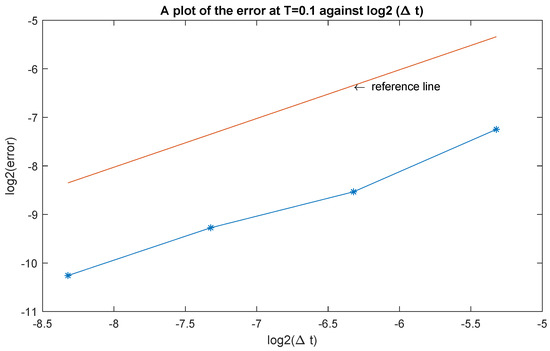
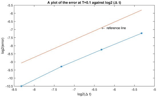
In Figure 1, we plot the experimentally determined orders of convergence with $\gamma =0.6$ and $\alpha =1.1$ as shown in Table 1 for the trace class noise. The expected convergence order is $O\left({\tau }^{min\{1,\alpha +\gamma -1/2\}}\right)=O\left(\tau \right)$. To get the plot, we choose the different time step sizes $\Delta t=(\Delta t_1,\Delta t_2,\Delta t_3,\Delta t_4)=2^{-2},2^{-3},2^{-4},2^{-5}$ and calculate the corresponding errors $y=(e_1,e_2,e_3,e_4)$. By error estimate we have $y\le C\Delta t^p$ with the convergence order $p>0$ which implies that

$$log2\left(y\right)\le log2\left(C\right)+plog2(\Delta t).$$

Figure 1. The experimentally determined orders of convergence with $\gamma =0.6$ and $\alpha =1.1$ in Table 1.

The reference line in Figure 1 is determined by four points $(log2(\Delta t_j),plog2(\Delta t_j)),j=1,2,3,4$ and the blue line in Figure 1 is determined by the four points $(log2(\Delta t_j),log2\left(e_j\right)),j=1,2,3,4$. If these two lines are parallel, then we may conclude that the experimentally determined convergence order is almost p. We use the similar approach to obtain other figures below.

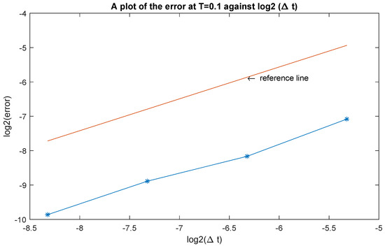
In Figure 2, we plot the experimentally determined orders of convergence with $\gamma =0.6$ and $\alpha =1.1$ as shown in Table 2 for the white noise. We observe that the convergence order is almost $O\left(\tau \right)$ in the figure, where the reference line represents the order $O\left(\tau \right)$.

Figure 2. The experimentally determined orders of convergence with $\gamma =0.6$ and $\alpha =1.1$ in Table 2.

Example 2.

Consider the following stochastic time fractional PDE, with $\alpha \in (1,2)$,

$$\begin{array}{cc}\hfill & {}_0^C{D}_t^{\alpha }u(t,x)-\frac{{\partial }^{2}u(t,x)}{\partial x^2}=f\left(u(t,x)\right)+g(t,x),0\le t\le T,0<x<1,\hfill \end{array}$$

(97)

$$\begin{array}{cc}\hfill & u(0,x)=u_0\left(x\right),\frac{\partial u(0,x)}{\partial t}=u_1\left(x\right),\hfill \end{array}$$

(98)

$$\begin{array}{cc}\hfill & u(t,0)=u(t,1)=0,\hfill \end{array}$$

(99)

where $f\left(u\right)=sin\left(u\right)$ and the initial values $u_0\left(x\right)=x^2{(1-x)}^2,u_1\left(x\right)=2x(1-x)(1-2x)$ and $g(t,x)$ is defined by (78).

We use the same notations as in Example 1. In Table 3, we consider the case of trace class noise, where ${\gamma }_m=m^{-2}$ for $m=1,2,\cdots$. We observe that the experimentally determined time convergence orders are consistent with our theoretical convergence orders, as indicated in the numbers in the brackets.

Table 3. Time convergence orders in Example 2 at $T=1$ with trace class noise ${\gamma }_m=m^{-2},m=1,2,\cdots$.

$\mathit{\alpha }$	$\mathit{\gamma }$	$\mathit{\tau }=1/4$	$\mathit{\tau }=1/8$	$1/16$	$1/32$	Order
$1.1$	0.0	1.48 × ${10}^{-2}$	8.28 × ${10}^{-3}$	4.96 × ${10}^{-3}$	2.77 × ${10}^{-3}$
			0.84	0.73	0.84	0.80 (0.60)
$1.1$	0.4	8.46 × ${10}^{-3}$	3.86 × ${10}^{-3}$	2.68 × ${10}^{-3}$	1.34 × ${10}^{-3}$
			1.13	0.52	0.99	0.88 (1.00)
$1.1$	0.6	6.57 × ${10}^{-3}$	2.69 × ${10}^{-3}$	1.61 × ${10}^{-3}$	8.16 × ${10}^{-4}$
			1.28	0.74	0.98	1.00 (1.00)
$1.1$	0.8	4.57 × ${10}^{-3}$	1.85 × ${10}^{-3}$	9.91 × ${10}^{-3}$	5.00 × ${10}^{-3}$
			1.30	0.90	0.98	1.06 (1.00)
$1.6$	0.0	1.32 × ${10}^{-2}$	5.77 × ${10}^{-3}$	3.18 × ${10}^{-3}$	1.54 × ${10}^{-3}$
			1.19	0.85	1.04	1.03 (1.00)
$1.6$	0.4	7.73 × ${10}^{-3}$	3.62 × ${10}^{-3}$	1.75 × ${10}^{-3}$	7.90 × ${10}^{-4}$
			1.09	1.04	1.15	1.09 (1.00)
$1.6$	0.6	6.64 × ${10}^{-3}$	3.24 × ${10}^{-3}$	1.55 × ${10}^{-3}$	6.77 × ${10}^{-4}$
			1.03	1.06	1.19	1.09 (1.00)
$1.6$	0.8	6.17 × ${10}^{-3}$	3.07 × ${10}^{-3}$	1.46 × ${10}^{-3}$	6.34 × ${10}^{-4}$
			1.00	1.06	1.20	1.09 (1.00)

In Table 4, we consider the case of white noise, where ${\gamma }_m=1$ for $m=1,2,\cdots$. We observe that the experimentally determined time convergence orders are slightly lower than the orders in the trace class noise case, as expected.

Table 4. Time convergence orders in Example 2 at $T=1$ with white noise ${\gamma }_m=1,m=1,2,\cdots$.

$\mathit{\alpha }$	$\mathit{\gamma }$	$\mathit{\tau }=1/4$	$\mathit{\tau }=1/8$	$1/16$	$1/32$	Order
$1.1$	0.0	6.57 × ${10}^{-2}$	4.86 × ${10}^{-2}$	3.60 × ${10}^{-2}$	2.36 × ${10}^{-2}$
			0.43	0.43	0.60	0.49
$1.1$	0.4	1.08 × ${10}^{-2}$	6.14 × ${10}^{-3}$	4.06 × ${10}^{-3}$	2.14 × ${10}^{-3}$
			0.81	0.59	0.92	0.77
$1.1$	0.6	7.38 × ${10}^{-3}$	3.48 × ${10}^{-3}$	2.11 × ${10}^{-3}$	1.07 × ${10}^{-3}$
			1.08	0.72	0.97	0.92
$1.1$	0.8	4.97 × ${10}^{-3}$	2.16 × ${10}^{-3}$	1.18 × ${10}^{-3}$	5.95 × ${10}^{-4}$
			1.19	0.87	0.99	1.02
$1.6$	0.0	2.70 × ${10}^{-2}$	1.64 × ${10}^{-2}$	1.02 × ${10}^{-2}$	5.58 × ${10}^{-3}$
			0.71	0.68	0.87	0.75
$1.6$	0.4	9.84 × ${10}^{-3}$	5.10 × ${10}^{-3}$	2.68 × ${10}^{-3}$	1.27 × ${10}^{-3}$
			0.94	0.92	1.07	0.98
$1.6$	0.6	7.40 × ${10}^{-3}$	3.72 × ${10}^{-3}$	1.83 × ${10}^{-3}$	8.17 × ${10}^{-4}$
			0.99	1.02	1.16	1.05
$1.6$	0.8	6.42 × ${10}^{-3}$	3.21 × ${10}^{-3}$	1.54 × ${10}^{-3}$	6.66 × ${10}^{-4}$
			0.99	1.05	1.20	1.08

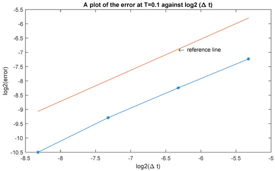
In Figure 3, we plot the experimentally determined orders of convergence with $\gamma =0.6$ and $\alpha =1.6$ for the trace class noise as shown in Table 3. The expected convergence order is $O\left({\tau }^{min\{1,\alpha +\gamma -1/2\}}\right)=O\left(\tau \right)$. The reference line in the figure represents the order $O\left(\tau \right)$, which is consistent with our observations.

Figure 3. The experimentally determined orders of convergence with $\gamma =0.6$ and $\alpha =1.6$ in Table 3.

In Figure 4, we plot the experimentally determined orders of convergence with $\gamma =0.6$ and $\alpha =1.6$ as shown in Table 4 for the white noise. We observe that the convergence order is almost $O\left(\tau \right)$ in the figure, where the reference line represents the order $O\left(\tau \right)$.

Figure 4. The experimentally determined orders of convergence with $\gamma =0.6$ and $\alpha =1.6$ in Table 4.

Example 3.

Consider the following stochastic time fractional PDE, with $\alpha \in (1,2)$,

$$\begin{array}{cc}\hfill & {}_0^C{D}_t^{\alpha }u(t,x)-\frac{{\partial }^{2}u(t,x)}{\partial x^2}=f\left(u(t,x)\right)+g(t,x),0\le t\le T,0<x<1,\hfill \end{array}$$

(100)

$$\begin{array}{cc}\hfill & u(0,x)=u_0\left(x\right),\frac{\partial u(0,x)}{\partial t}=u_1\left(x\right),\hfill \end{array}$$

(101)

$$\begin{array}{cc}\hfill & u(t,0)=u(t,1)=0,\hfill \end{array}$$

(102)

where $f\left(u\right)=-u^3+u$ and the initial values $u_0\left(x\right)=x^2{(1-x)}^2,u_1\left(x\right)=2x(1-x)(1-2x)$ and $g(t,x)$ are defined by (78).

We use the same notations as in Example 1. In Table 5, we consider the trace class noise, i.e., ${\gamma }_m=m^{-2},m=1,2,\cdots$, and observe that the experimentally determined time convergence orders are consistent with our theoretical convergence orders. The numbers in the brackets denote the theoretical convergence orders.

Table 5. Time convergence orders in Example 3 at $T=1$ with trace class noise ${\gamma }_m=m^{-2},m=1,2,\cdots$.

$\mathit{\alpha }$	$\mathit{\gamma }$	$\mathit{\tau }=1/4$	$\mathit{\tau }=1/8$	$1/16$	$1/32$	Order
$1.1$	0.0	1.91 × ${10}^{-2}$	1.07 × ${10}^{-2}$	6.75 × ${10}^{-3}$	3.74 × ${10}^{-3}$
			0.82	0.67	0.84	0.78 (0.60)
$1.1$	0.4	1.15 × ${10}^{-2}$	5.24 × ${10}^{-3}$	3.32 × ${10}^{-3}$	1.62 × ${10}^{-3}$
			1.13	0.65	1.03	0.94 (1.00)
$1.1$	0.6	1.01 × ${10}^{-2}$	4.53 × ${10}^{-3}$	2.42 × ${10}^{-3}$	1.16 × ${10}^{-3}$
			1.15	0.90	1.05	1.03 (1.00)
$1.1$	0.8	8.50 × ${10}^{-3}$	3.94 × ${10}^{-3}$	1.93 × ${10}^{-3}$	9.04 × ${10}^{-4}$
			1.10	1.03	1.09	1.07 (1.00)
$1.6$	0.0	1.38 × ${10}^{-2}$	6.34 × ${10}^{-3}$	3.50 × ${10}^{-3}$	1.68 × ${10}^{-3}$
			1.12	0.85	1.05	1.01 (1.00)
$1.6$	0.4	7.77 × ${10}^{-3}$	3.70 × ${10}^{-3}$	1.82 × ${10}^{-3}$	8.08 × ${10}^{-4}$
			1.06	1.02	1.17	1.08 (1.00)
$1.6$	0.6	6.74 × ${10}^{-3}$	3.33 × ${10}^{-3}$	1.61 × ${10}^{-3}$	6.98 × ${10}^{-4}$
			1.01	1.04	1.21	1.09 (1.00)
$1.6$	0.8	6.35 × ${10}^{-3}$	3.20 × ${10}^{-3}$	1.54 × ${10}^{-3}$	6.62 × ${10}^{-4}$
			0.98	1.05	1.22	1.08 (1.00)

In Table 6, we consider the white noise, i.e., ${\gamma }_m=1,m=1,2,\cdots$, and observe that the experimentally determined time convergence orders are slightly less than the orders in the trace class noise case, as expected.

Table 6. Time convergence orders in Example 3 at $T=1$ with white noise ${\gamma }_m=1,m=1,2,\cdots$.

$\mathit{\alpha }$	$\mathit{\gamma }$	$\mathit{\tau }=1/4$	$\mathit{\tau }=1/8$	$1/16$	$1/32$	Order
$1.1$	0.0	6.58 × ${10}^{-2}$	4.86 × ${10}^{-2}$	3.61 × ${10}^{-2}$	2.37 × ${10}^{-2}$
			0.43	0.43	0.60	0.49
$1.1$	0.4	1.32 × ${10}^{-2}$	6.99 × ${10}^{-3}$	4.45 × ${10}^{-3}$	2.29 × ${10}^{-3}$
			0.92	0.65	0.95	0.84
$1.1$	0.6	1.06 × ${10}^{-2}$	5.00 × ${10}^{-3}$	2.75 × ${10}^{-3}$	1.34 × ${10}^{-3}$
			1.08	0.86	1.03	0.99
$1.1$	0.8	8.71 × ${10}^{-3}$	4.08 × ${10}^{-3}$	2.02 × ${10}^{-3}$	5.56 × ${10}^{-4}$
			1.09	1.01	1.08	1.06
$1.6$	0.0	2.69 × ${10}^{-2}$	1.64 × ${10}^{-2}$	1.02 × ${10}^{-2}$	5.57 × ${10}^{-3}$
			0.70	0.68	0.87	0.75
$1.6$	0.4	9.71 × ${10}^{-3}$	5.07 × ${10}^{-3}$	2.68 × ${10}^{-3}$	1.26 × ${10}^{-3}$
			0.93	0.91	1.08	0.98
$1.6$	0.6	7.41 × ${10}^{-3}$	3.75 × ${10}^{-3}$	1.87 × ${10}^{-3}$	8.25 × ${10}^{-4}$
			0.97	1.00	1.18	1.05
$1.6$	0.8	6.55 × ${10}^{-3}$	3.31 × ${10}^{-3}$	1.60 × ${10}^{-3}$	6.90 × ${10}^{-4}$
			0.98	1.04	1.22	1.08

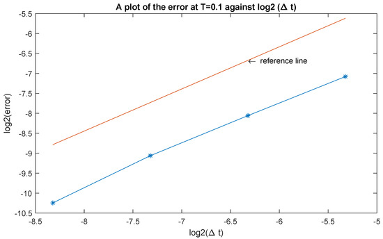
In Figure 5, we plot the experimentally determined orders of convergence with $\gamma =0.6$ and $\alpha =1.6$ in Table 5 for the trace class noise. The expected convergence order is $O\left({\tau }^{min\{1,\alpha +\gamma -1/2\}}\right)=O\left(\tau \right)$. We indeed observe this in the figure where the reference line is for the order $O\left(\tau \right)$.

Figure 5. The experimentally determined orders of convergence with $\gamma =0.6$ and $\alpha =1.6$ in Table 5.

In Figure 6, we plot the experimentally determined orders of convergence with $\gamma =0.6$ and $\alpha =1.6$ in Table 6 for the white noise. We observe that the convergence order is almost $O\left(\tau \right)$ in the figure where the reference line is for the order $O\left(\tau \right)$.

Figure 6. The experimentally determined orders of convergence with $\gamma =0.6$ and $\alpha =1.6$ in Table 6.

7. Conclusions

In this paper, we explore a numerical approach to approximate the stochastic semilinear space–time fractional wave equation. We establish the existence of a unique solution for this equation by using the Banach fixed point theorem, assuming that the nonlinear function satisfies the global Lipschitz condition. To obtain the stochastic regularized problem, we approximate the noise using a piecewise constant function in time. The finite element method is then employed to approximate the stochastic regularized problem. Furthermore, we propose a natural extension of this work, which involves considering more general nonlinear functions, such as the Allen–Cahn equation, as well as exploring different types of noise, including fractional noise with a Hurst parameter $H\in (0,1)$. Additionally, it might be very interesting to investigate more advanced fractal–fractional derivatives [30] in our stochastic space–time fractional wave equation.

Appendix A.1. Calculate the kth Element of (f(u(t_n)),φ_k) in Fⁿ in (90)

 % find (fu, phi)

    function y=fu_phi(x,n,tau,alpha,v,Ph_u0,Ph_u1)

       tn=n∗tau;

       h=x(2)-x(1);

       U0=v+Ph_u0+tn∗Ph_u1;

       U_1=[0;U0(1:end-1)];

       U1=[U0(2:end);0];

       % f(u)= sin(u)

       F0=sin(U0); F_1=sin(U_1); F1=sin(U1);

       y=h/4∗(F_1+2∗F0+F1);

Appendix A.2. Generate the Fractional Brownian Motions ${\beta }_m^H$ (t₀), ${\beta }_m^H$ (t₁),⋯ ${\beta }_m^H$(t_N), m = 1, 2, ⋯, M − 1 with the Hurst Number H ∈ [1/2,1]

.

     W=[];

     for j=1:M-1

         [Wj,t]=fbm1d(H,Nref,T);

         W=[W Wj];

     end

     W(1,:)=zeros(1, M-1);

Appendix A.3. Caculating gⁿ (l) in (91)

 % find (g, phi)

    function y=g_phi(x,n,tau,ga,kappa,W)

        y=[];

        M=length(x)+1;

        %Find w_ga=[w_{0}^{-ga} w_{1}^{-ga}  w_{n-1}^{-ga}]

        w_ga=[];

        for nn=0:n-1

            w_ga=[w_ga w_gru(nn,-ga)];

        end

        for k=1:M-1

            A=dWdt_k(x,n,tau,kappa,W,k);

            y1=tau^(ga)∗w_ga∗A;

            y=[y;y1];

        end

    % Find dWdt_k

 function y= dWdt_k(x,n,tau,kappa,W,k)

        y=zeros(n,1);

        M=length(x)+1;

        for m=1:M-1

            beta=2; % white noise beta=0, trace class beta=2

            ga_m=m^(-beta);

            k1=n:-1:1;  %tn=n∗tau=(n∗kappa)∗dtref

            dW_k1=W(k1∗kappa+1,m)-W((k1-1)∗kappa+1,m); %dW_k is a vector

            h=x(2)-x(1);

            x1=((k-1)∗h+k∗h)/2; x2= (k∗h+(k+1)∗h)/2;

            e_phi=h/2∗(sqrt(2)∗sin(pi∗m∗x1)+sqrt(2)∗sin(pi∗m∗x2));

            y=y+ga_m^(1/2)∗e_phi∗(dW_k1/tau);

        end

References

- Meerschaert, M.M.; Schilling, R.L.; Sikorskii, A. Stochastic solutions for fractional wave equations. Nonlinear Dynam. 2015, 80, 1685–1695. [Google Scholar] [CrossRef] [PubMed]
- Chen, W.; Holm, S. Fractional Laplacian time-space models for linear and nonlinear lossy media exhibiting arbitrary frequency power-law dependency. J. Acoust. Soc. Am. 2004, 115, 1424–1430. [Google Scholar] [CrossRef] [PubMed]
- Szabo, T.L. Time domain wave equations for lossy media obeying a frequency power law. J. Acoust. Soc. Am. 1994, 96, 491–500. [Google Scholar] [CrossRef]
- Chen, Z.Q.; Kim, K.H.; Kim, P. Fractional time stochastic partial differential equations. Stoch. Process. Appl. 2015, 125, 1470–1499. [Google Scholar] [CrossRef]
- Li, Y.; Wang, Y.; Deng, W. Galerkin finite element approximations for stochastic space-time fractional wave equations. SIAM J. Numer. Anal. 2017, 55, 3173–3202. [Google Scholar] [CrossRef]
- Li, Y.; Wang, Y.; Deng, W.; Nie, D. Galerkin finite element approximation for semilinear stochastic time-tempered fractional wave equations with multiplicative Gaussian noise and additive fractional Gaussian noise. Numer. Math. Theory Methods Appl. 2022, 15, 1063–1098. [Google Scholar] [CrossRef]
- Chen, G.G.; Duan, J.Q.; Zhang, J. Approximating dynamics of a singularity perturbed stochastic wave equation with a random dynamical boundary condition. SIAM J. Math. Anal. 2012, 45, 2790–2814. [Google Scholar] [CrossRef]
- Anh, V.V.; Leonenko, N.N.; Ruiz-Medina, M. Space-time fractional stochastic equations on regular bounded open domains. Fract. Calc. Appl. Anal. 2016, 19, 1161–1199. [Google Scholar] [CrossRef]
- Chen, L. Nonlinear stochastic time-fractional diffusion equations on : Moments. Hölder regularity and intermittency. Approximating dynamics of a singularity perturbed stochastic wave equation with a random dynamical boundary condition. Trans. Am. Math. Soc. 2017, 369, 8497–8535. [Google Scholar] [CrossRef]
- Chen, L.; Hu, Y.; Nualart, D. Nonlinear stochastic time-fractional slow and fast diffusion equations on . Stoch. Process. Appl. 2019, 129, 5073–5112. [Google Scholar] [CrossRef]
- Liu, W.; Röckner, M.; Da Silva, J.L. Quasi-linear (stochastic) partial differential equations with time-fractional derivatives. Stoch. Process. Appl. 2019, 129, 5073–5112. [Google Scholar] [CrossRef]
- Thach, T.N.; Tuan, N.H. Stochastic pseudo-parabolic equations with fractional derivative and fractional Brownian motion. Stoch. Anal. Appl. 2022, 40, 328–351. [Google Scholar] [CrossRef]
- Balan, R.M.; Tudor, C.A. The stochastic wave equation with fractional noise: A random field approach. Stoch. Process. Appl. 2010, 120, 2468–2494. [Google Scholar] [CrossRef]
- Jin, B.; Yan, Y.; Zhou, Z. Numerical approximation of stochastic time-fractional diffusion. ESAIM Math. Model. Numer. Anal. 2019, 53, 1245–1268. [Google Scholar] [CrossRef]
- Qi, R.; Wang, X. Error estimates of semidiscrete and fully discrete finite element methods for the Cahn-Hilliard-Cook equation. SIAM J. Numer. Anal. 2020, 58, 1613–1653. [Google Scholar] [CrossRef]
- Li, S.; Cao, W. On spectral Petrov–Galerkin method for solving optimal control problem governed by fractional diffusion equations with fractional noise. J. Sci. Comput. 2023, 94, 62. [Google Scholar] [CrossRef]
- Al-Maskari, M.; Karaa, S. Strong convergence rates for the approximation of a stochastic time-fractional Allen–Cahn equation. Commun. Nonlinear Sci. Numer. Simul. 2023, 119, 107099. [Google Scholar] [CrossRef]
- Balan, R.M. The stochastic wave equation with multiplicative fractional noise: A Malliavin calculus approach. Potential Anal. 2012, 36, 1–34. [Google Scholar] [CrossRef]
- Wang, X.; Gan, S.; Tang, J. Higher order strong approximations of semilinear stochastic wave equation with additive space-time white noise. SIAM J. Sci. Comput. 2014, 36, A2611–A2632. [Google Scholar] [CrossRef]
- Anton, R.; Cohen, D.; Larsson, S. Wang, X. Full discretization of semilinear stochastic wave equations driven by multiplicative noise. SIAM J. Numer. Anal. 2016, 54, 1093–1119. [Google Scholar] [CrossRef]
- Zhou, Y.; Wang, Q.; Zhang, Z. Physical properties preserving numerical simulation of stochastic fractional nonlinear wave equation. Commun. Nonlinear Sci. Numer. Simul. 2021, 99, 105832. [Google Scholar] [CrossRef]
- Alshammari, S.; Al-Sawalha, M.M.; Shah, R. Approximate analytical methods for a fractional-order nonlinear system of Jaulent–Miodek equation with energy-dependent Schrödinger potential. Fractal Fract. 2023, 7, 140. [Google Scholar] [CrossRef]
- Shah, N.A.; Hamed, Y.S.; Abualnaja, K.M.; Chung, J.D.; Shah, R.; Khan, A. A comparative analysis of fractional-order Kaup–Kupershmidt equation within different operators. Symmetry 2022, 14, 986. [Google Scholar] [CrossRef]
- Shah, N.A.; Alyousef, H.A.; El-Tantawy, S.A.; Shah, R.; Chung, J.D. Analytical investigation of fractional-order Korteweg–De-Vries-type equations under Atangana–Baleanu–Caputo operator: Modeling nonlinear waves in a plasma and fluid. Symmetry 2022, 14, 739. [Google Scholar] [CrossRef]
- Al-Sawalha, M.M.; Ababneh, O.Y.; Shah, R.; Shah, N.A.; Nonlaopon, K. Combination of Laplace transform and residual power series techniques of special fractional-order non-linear partial differential equations. AIMS Math. 2023, 8, 5266–5280. [Google Scholar] [CrossRef]
- Noor, S.; Alshehry, A.S.; Aljahdaly, N.H.; Dutt, H.M.; Khan, I.; Shah, R. Investigating the impact of fractional non-linearity in the Klein–Fock–Gordon equation on quantum dynamics. Symmetry 2023, 15, 881. [Google Scholar] [CrossRef]
- El-Tantawy, S.A.; Shah, R.; Alrowaily, A.W.; Shah, N.A.; Chung, J.D.; Ismaeel, S.M. A comparative study of the fractional-order Belousov–Zhabotinsky system. Mathematics 2023, 11, 1751. [Google Scholar] [CrossRef]
- Kang, W.; Eqwu, B.A.; Yan, Y. Galerkin finite element approximation of a stochastic semilinear fractional subdiffusion with fractionally integrated additive noise. IMA J. Numer. Anal. 2022, 42, 2301–2335. [Google Scholar] [CrossRef]
- Botev, Z.; Fractional Brownian Motion Generator. MATLAB Central File Exchange. Available online: https://www.mathworks.com/matlabcentral/fileexchange/38935-fractional-brownian-motion-generator (accessed on 20 June 2016).
- Youssri, Y.H.; Atta, A.G. Spectral collocation approach via normalized shifted Jacobi polynomials for the nonlinear Lane-Emden Equation with fractal-fractional derivative. Fractal Fract. 2023, 7, 133. [Google Scholar] [CrossRef]
Disclaimer/Publisher’s Note: The statements, opinions and data contained in all publications are solely those of the individual author(s) and contributor(s) and not of MDPI and/or the editor(s). MDPI and/or the editor(s) disclaim responsibility for any injury to people or property resulting from any ideas, methods, instructions or products referred to in the content. |
© 2023 by the authors. Licensee MDPI, Basel, Switzerland. This article is an open access article distributed under the terms and conditions of the Creative Commons Attribution (CC BY) license (https://creativecommons.org/licenses/by/4.0/).