On Fractional Lyapunov Functions of Nonlinear Dynamic Systems and Mittag-Leffler Stability Thereof

Abstract

In this paper, fractional Lyapunov functions for epidemic models are introduced and the concept of Mittag-Leffler stability is applied. The global stability of the epidemic model at an equilibrium state is established.

1. Introduction

In a nonlinear fractional-order system, the Lyapunov direct method can be used to research the Mittag-Leffler stability without having to solve the fractional differential equations directly [1,2]. This technique broadens the idea of demonstrating that a model is stable if it contains any Lyapunov function possibility [3]. It can be used to measure the size of a basin of attraction or the rate at which critical point techniques are applied. It has also been used in the proof of the Hopf-type bifurcation theorem [4]. This approach has been extensively used by many mathematicians in the study of dynamical systems [5,6,7]. Many authors provided Lyapunov for the $SIR$ epidemic model in [8,9]. Further, it was generalized and applied to multicompartment mathematical models with nonlinear functional answers [10,11,12].

The fractional-order calculus is related to models with the concept of memory in the communicable disease [13]. The stability analysis of the epidemic model with different biological parameters has been obtained [14]. We extended the work of author [15] by constructing the Lyapunov function for $SIR$ and $SIRS$ models for fractional-order dynamical systems. Lyapunov is a tool, if such an operator exists, for analyzing the global stability in nonlinear dynamical systems. If the Lyapunov function exists for a given nonlinear dynamical system, then the system is stable.

The paper is organized as follows: The basic preliminary of fractional calculus is given in Section 2. The model is described in Section 3. Mittag-Leffler stability analysis is discussed in Section 4. Numerical simulations are presented in Section 5. Finally, the conclusion is drawn in Section 6.

2. Basic Preliminary

In this section, we present some basic definitions of fractional calculus that are used in this paper, as fractional calculus plays a vital role in applied science and engineering. Here, we discuss the fractional integral and derivatives of the Riemann–Liouville and Caputo operators.

Definition 1

([16]). The Riemann–Liouville fractional integral of the function f is defined as

$$\begin{array}{cc}\hfill {}_{t_0}^{RL}{D}_t^{-\alpha }f\left(t\right)=& {\displaystyle \frac{1}{\Gamma \left(\alpha \right)}{\int }_{t_0}^t{(t-v)}^{\alpha -1}f\left(v\right)dv,\alpha \in {\mathbb{R}}^{+}.}\hfill \end{array}$$

(1)

Definition 2

([16]). The Riemann–Liouville fractional derivative of the function f is defined as

$$\begin{array}{cc}\hfill {}_{t_0}^{RL}{D}_t^{\alpha }f\left(t\right)=& {\displaystyle \frac{1}{\Gamma (n-\alpha )}\frac{d^n}{d{t}^n}{\int }_{t_0}^t{(t-v)}^{n-\alpha -1}f\left(v\right)dv,t>0,\alpha \in [n-1,n),n\in {\mathbb{Z}}^{+}.}\hfill \end{array}$$

(2)

Remark 1.

If $\alpha \in \mathbb{R}$ and $v>-1$, then ${\displaystyle {}_{t_0}^{RL}{D}_t^{\alpha }{(t-t_0)}^v=\frac{\Gamma (1+v)}{\Gamma (1-\alpha )}.}$

Definition 3

([16]). The Caputo fractional derivative of the function f is defined as

$$\begin{array}{cc}\hfill {}_{t_0}^C{D}_t^{\alpha }f\left(t\right)=& {\displaystyle \frac{1}{\Gamma (n-\alpha )}{\int }_{t_0}^t{(t-v)}^{n-\alpha -1}{f}^{\left(n\right)}\left(v\right)dv,\alpha \in (n-1,n),n\in {\mathbb{Z}}^{+}.}\hfill \end{array}$$

(3)

The Mittag-Leffler function is the development of the exponential function.

Definition 4

([17]). The one-parametric Mittag-Leffler function of g is defined as

$$\begin{array}{cc}\hfill E_{a_1}\left(g\right)=& {\displaystyle \sum _{k=0}^{\infty }\frac{g^k}{\Gamma (\alpha k+1)},Re\left(a_1\right)>0,g\in \mathbb{C}.}\hfill \end{array}$$

(4)

Definition 5

([17]). The two-parametric Mittag-Leffler function of g is defined as

$$\begin{array}{cc}\hfill E_{a_1,a_2}\left(g\right)=& {\displaystyle \sum _{k=0}^{\infty }\frac{g^k}{\Gamma (a_{1}k+a_2)},Re\left(a_1\right)>0,a_2,g\in \mathbb{C}.}\hfill \end{array}$$

(5)

Remark 2.

If $a_2=1$, then Equation $\left(5\right)$ yields $E_{a_1,1}\left(g\right)=E_{a_1}\left(g\right).$ In particular, if $a_1=a_2=1$, then $E_{1,1}\left(g\right)=E_1\left(g\right)=e^x.$

Remark 3.

The relationship between Mittag-Leffler and the gamma function is given as

$$\begin{array}{cc}\hfill E_{a_1,a_2}\left(g\right)=& {\displaystyle g{E}_{a_1,a_1+a_2}\left(g\right)+\frac{1}{\Gamma \left(a_2\right)}.}\hfill \end{array}$$

(6)

Remark 4.

The Laplace transformation of the two-parametric Mittag-Leffler function is

$$\begin{array}{cc}\hfill \mathcal{L}\left\{t^{a_2-1}{E}_{a_1,a_2}(-\hslash t^{a_1})\right\}=& {\displaystyle \frac{r^{a_1-a_2}}{r^{a_1}+\hslash },t\ge 0,Re\left(r\right)>{|\hslash |}^{1/a_1},\hslash \in \mathbb{R}.}\hfill \end{array}$$

(7)

3. Model Description

In this section, the susceptible class S, the infected class I, and the recovered class R are the three distinct classes that make up the total population Z. When susceptible individuals contract the illness after coming into contact with an infectious person, the individuals joins the infected class and, eventually, as a consequence of isolation or recovery, the removed compartment. If a recovered population preserves their immunity indefinitely, after that they will stay in the recovered compartment. This is the foundation of the $SIR$ model. In addition, it is thought that all progeny are recruited healthy and are placed in the susceptible section. Assume that the inscription of recruitment into the person is proportional to its size Z and that the spread of infection occurs according to the law of mass action. The $SIR$ model can now be decomposed into the following system of ordinary differential equations:

$$\begin{array}{cc}\hfill \dot{S}=& \mathrm{\Delta }Z-\eta SI/Z-\mu S,\hfill \\ \hfill \dot{I}=& \eta SI/Z-(d+{\mu }_1+\mu )I,\hfill \\ \hfill \dot{R}=& dI-\mu R,\hfill \end{array}$$

(8)

where $\mathrm{\Delta }$ is the recruitment rate, $\eta$ is the rate of prevalence, $\mu$ is the natural mortality charge, d is the recovery charge, and ${\mu }_1$ the disease-induced death charge. All of these biological parameters must be non-negative.

This $SIR$ model may be generalized further to account for temporary immunity, in which candidates of the R class can lose their temporary immunity along time and go back to the S class. The $SIRS$ model is a product of this sort of extension. In addition, the vertical transmission consists of supposing that a biological parameter f of the offspring is infected at recruitment and joins the ineffective class [18]. Using these conditions and the charge of loss of immunity by $\omega$, the $SIR$ model can be written as below in terms of equations:

$$\begin{array}{cc}\hfill \dot{S}=& \mathrm{\Delta }(Z-fI)-\eta SI/Z-\mu S+\omega R,\hfill \\ \hfill \dot{I}=& f\mathrm{\Delta }I+\eta SI/Z-(d+{\mu }_1+\mu )I,\hfill \\ \hfill \dot{R}=& dI-(\mu +\omega )R.\hfill \end{array}$$

(9)

Under the condition that Z is constant, the $SIR$ and $SIRS$ models can be reduced to a two-dimensional model. Traditionally, the mathematical statement for the recovered class $R\left(t\right)$ is not included. When Z is constant, the first and second mathematical statements of the system $\left(8\right)$ can be easily decoupled. To find R, use the assumption $Z=S+I+R$ = constant. The mathematical statements for $S\left(t\right)$ and $I\left(t\right)$ cannot be included, but ignoring the mathematical statement for $R\left(t\right)$ seems backward. Furthermore, by not including the mathematical statement for $S\left(t\right)$ instead of $R\left(t\right)$, it is possible to make both the epidemic $SIR$ and $SIRS$ models equivalent for the outcome of a two-dimensional system, including epidemic systems with the vertical dynamical transmission. Thus, the two-dimensional model is as below.

$$\begin{array}{cc}\hfill \dot{I}=& \left({\aleph }_1(Z-I-R)-\delta \right)I,\hfill \\ \hfill \dot{R}=& dI-{\aleph }_{2}R,\hfill \end{array}$$

(10)

where ${\aleph }_1=\eta /Z,{\aleph }_2=\mu +\omega ,and\delta =d+{\mu }_1+\mu -f\mathrm{\Delta }$. Let $g=\eta Z-\omega$, We have the ability to rewrite the system $\left(10\right)$ as

$$\begin{array}{cc}\hfill \dot{I}=& (g-\eta I-\eta R)I,\hfill \\ \hfill \dot{R}=& dI-\mu R.\hfill \end{array}$$

(11)

There are multiple definitions of fractional derivatives and integrals in fractional calculus [19], but in this work, system $\left(11\right)$ is based on the Caputo derivative [20]. Therefore, we have

$$\begin{array}{cc}\hfill {}_0^C{D}_t^{\alpha }I=& (g-\eta I-\eta R)I,\hfill \\ \hfill {}_0^C{D}_t^{\alpha }R=& dI-\mu R.\hfill \end{array}$$

(12)

where $\alpha \in (0,1)$. Let $E_0=(I_0,R_0)=(0,0)$ be the free critical point of system $\left(12\right)$, and $E_1=(I_1,R_1)=(\mu g/\eta (d+\mu ),dg/\eta (d+\mu ))$ be the endemic critical point of system $\left(12\right)$. Further, it can be seen that the $E_0$ exists when ${\mathcal{R}}_0=\eta Z/\sigma >1.$ At the critical point, the expressions $g=\eta (I_1+R_1)$ and $d{I}_1-\mu R_1$ both hold. Inputting these two expressions into system $\left(12\right)$, we have the system $\left(12\right)$ as a skew-symmetric form.

$$\begin{array}{cc}\hfill {}_0^C{D}_t^{\alpha }I=& I(\eta (I_1-I)+\eta (R_1-R)),\hfill \\ \hfill {}_0^C{D}_t^{\alpha }R=& \mu (R_1-R)-d(I_1-I).\hfill \end{array}$$

(13)

4. Mittag-Leffler Stability

In this section, we express the stability in Mittag-Leffler’s perspective.

Definition 6

([1]). The solution of system $\left(12\right)$ is called the Mittag-Leffler stable if

$$\begin{array}{cc}\hfill \parallel y\left(t\right)\parallel \le & {\left\{m\left[y\left(t_0\right)\right]E_{a_1}{(-\hslash (t-t_0))}^{a_1}\right\}}^b,\hfill \end{array}$$

(14)

where $y=(I,R)$, $a_1\in (0,1)$, $b>0$, $\hslash \ge 0$, $m\left(0\right)=0,$   $t_0$ is the initial time, $m\left(y\right)\ge 0$ and $m\left(y\right)$ is locally Lipschitz on $y\in \mathbb{B}\in {\mathbb{R}}^n$ with Lipschitz constant $m_0$.

Definition 7

([21]). The explanation of system $\left(12\right)$ is known as generalized Mittag-Leffler stability if

$$\begin{array}{cc}\hfill \parallel y\left(t\right)\parallel \le & {\left\{m\left[y\left(t_0\right)\right]{(t-t_0)}^{-\theta }{E}_{a_1,1-\theta }{(-\hslash (t-t_0))}^{a_1}\right\}}^b,\hfill \end{array}$$

(15)

where $a_1\in (0,1)$, $\theta \in (-a_1,1-a_1]$, $b>0$, $\hslash \ge 0$, $m\left(0\right)=0,$   $m\left(y\right)\ge 0,$ and $m\left(y\right)$ is locally Lipschitz on $y\in \mathbb{B}\in {\mathbb{R}}^n$ with Lipschitz constant $m_0$.

The two aforementioned stabilities imply asymptotic stability. The asymptotic stability of the model $\left(12\right)$ can be obtained using the Lyapunov second method. We now apply this technique to the system $\left(12\right)$, resulting in Mittag-Leffler stability.

Remark 5.

If $\hslash =0$, then Equation $\left(15\right)$ gives

$$\begin{array}{cc}\hfill \parallel y\left(t\right)\parallel \le & {\left[m\left(y\left(t_0\right)\right)/\Gamma (1-\theta )\right]}^b{(t-t_0)}^{-\theta b}.\hfill \end{array}$$

(16)

Equation $\left(16\right)$ implies that power-law stability is an exceptional point of Mittag-Leffler stability.

Remark 6.

The below two conditions are comparable:

(i) 

$m\left(y\right)$is Lipschitz in regard to y.

(ii) 

∃$m_0$ satisfying $\parallel m\left(I\right)-m\left(R\right)\parallel \le m_0\parallel I-R\parallel ,$ and if $R=0,$ then $\parallel m\left(I\right)\parallel \le m_0\parallel I\parallel .$

Theorem 1.

Let $y=0$ be the critical point of the system $\left(12\right)$ and the domain with origin is a subset of ${\mathbb{R}}^n.$ If $V(t,y(t\left)\right):[0,\infty )\times \mathbb{D}\to \mathbb{R}$ is the continuous differentiable mapping as well as locally Lipschitz in regard to y such that

$$\begin{array}{cc}\hfill {\sigma }_1{\parallel y\parallel }^{c_1}\le V(t,y\left(t\right)) \le & {\sigma }_2{\parallel y\parallel }^{c_1{c}_2},\hfill \end{array}$$

(17)

$$\begin{array}{cc}\hfill {}_0^C{D}_t^{\alpha }V(t,y\left(t\right)) \le & -{\sigma }_3{\parallel y\parallel }^{c_1{c}_2}\hfill \end{array}$$

(18)

where t is positive, $y\in \mathbb{D}$, $\alpha \in (0,1)$, ${\sigma }_1,{\sigma }_2,{\sigma }_3,c_1$&$c_2$ are constants. Then $y=0$ is Mittag-Leffler stable. In addition, if the above conditions grasp globally on ${\mathbb{R}}^n$, then $y=0$ is globally Mittag-Leffler stable.

Proof. 

From the above Equations $\left(17\right)$ and $\left(18\right)$, we have

$$\begin{array}{cc}\hfill {}_0^C{D}_t^{\alpha }V(t,y\left(t\right)) \le & {\displaystyle -\frac{{\sigma }_3}{{\sigma }_2}V(t,y\left(t\right)).}\hfill \end{array}$$

There exists a positive function $G\left(t\right)$ satisfying

$$\begin{array}{cc}\hfill {}_0^C{D}_t^{\alpha }V(t,y\left(t\right))+G\left(t\right)=& {\displaystyle -\frac{{\sigma }_3}{{\sigma }_2}V(t,y\left(t\right)).}\hfill \end{array}$$

(19)

On taking the Laplace both sides of the Equation $\left(19\right),$ we have

$$\begin{array}{cc}\hfill r^{\alpha }V\left(r\right)-V\left(0\right)r^{\alpha -1}+G\left(r\right)=& {\displaystyle -\frac{{\sigma }_3}{{\sigma }_2}V\left(r\right),}\hfill \end{array}$$

(20)

where $V\left(0\right)$ is equal to $V(0,y(0\left)\right)$ and $V\left(r\right)=\mathcal{L}\left(r\right)=\mathcal{L}\left\{V\right(t,y\left(t\right)\left)\right\}$ are positive constants. From Equation $\left(20\right)$, we obtain

$$\begin{array}{cc}\hfill V\left(r\right)=& {\displaystyle \frac{V\left(0\right)r^{\alpha -1}-G\left(r\right)}{r^{\alpha }+\frac{{\sigma }_3}{{\sigma }_2}}.}\hfill \end{array}$$

If $y\left(0\right)=0$, such that $V\left(0\right)=0,$ the value to the system $\left(12\right)$ is $y=0$.

If $y\left(0\right)=0$, such that $V\left(0\right)$ is positive, from $V(t,y)$, “Theorem 3.7” of [21], and the Laplace inverse transformation of Equation $\left(19\right)$, it gives

$$\begin{array}{cc}\hfill V\left(t\right)=& {\displaystyle V\left(0\right)E_{a_1}\left(-\frac{{\sigma }_3}{{\sigma }_2}{t}^{a_1}\right)-G\left(t\right)\left[t^{a_1-1}{E}_{a_1,a_1}\left(-\frac{{\sigma }_3}{{\sigma }_2}{t}^{a_1}\right)\right].}\hfill \end{array}$$

Since both the functions $t^{a_1-1}$ and ${\displaystyle E_{a_1,a_1}\left(-\frac{{\sigma }_3}{{\sigma }_2}{t}^{a_1}\right)}$ are positive, we have

$$\begin{array}{cc}\hfill V\left(t\right) \le & {\displaystyle V\left(0\right)E_{a_1}\left(-\frac{{\sigma }_3}{{\sigma }_2}{t}^{a_1}\right).}\hfill \end{array}$$

(21)

Inputting Equation $\left(21\right)$ into $\left(17\right)$, we get

$$\begin{array}{cc}\hfill \parallel y\left(t\right)\parallel \le & {\displaystyle {\left[\frac{V\left(0\right)}{{\sigma }_1}{E}_{a_1}{t}^{\alpha -1}{E}_{a_1,a_1}\left(-\frac{{\sigma }_3}{{\sigma }_2}{t}^{a_1}\right)\right]}^{\frac{1}{c_1}},}\hfill \end{array}$$

where ${\displaystyle \frac{V\left(0\right)}{{\sigma }_1}>0}$ for $y\left(0\right)=0.$

Letting ${\displaystyle m=\frac{V\left(0\right)}{{\sigma }_1}=\frac{V(0,y(0\left)\right)}{{\sigma }_1}\ge 0,}$ we have

$$\begin{array}{cc}\hfill \parallel y\left(t\right)\parallel \le & {\displaystyle {\left[m{E}_{a_1}\left(-\frac{{\sigma }_3}{{\sigma }_2}{t}^{a_1}\right)\right]}^{\frac{1}{c_1}},}\hfill \end{array}$$

where $m=0$ grasps iff $y\left(0\right)$ is equal to zero. Therefore $V(t,y)$, the local Lipschitz condition, $V(0,y(0\left)\right)=0$ iff $y\left(0\right)$ is also equal to zero, so $m\left(0\right)=0$ and ${\displaystyle m=\frac{V(0,y(0\left)\right)}{{\sigma }_1}}$ is also Lipschitz, and this means the stability of Equation $\left(12\right).$ □

Theorem 2.

In “Theorem 1", there exists a $t_1$ corresponding to the equilibria $y=0$, which is generalized Mittag-Leffler stability for $t\ge t_1.$

Proof. 

From the proof of “Theorem 1” ∃ a $G\left(r\right)$ satisfying Equation $\left(20\right)$. Let $\mathcal{L}\left\{\tilde{G}\left(t\right)\right\}=\tilde{G}\left(r\right)=G\left(r\right)-V\left(0\right)r^{a_1-1}+V\left(0\right)r^{a_1-\widetilde{a_1}},$ where $a_1 \le \widetilde{a_1}<1+a_1,$ we have

$$\begin{array}{cc}\hfill V\left(r\right)=& {\displaystyle \frac{V\left(0\right)r^{a_1-\widetilde{a_1}}-\tilde{G}\left(r\right)}{r^{a_1}+\frac{{\sigma }_3}{{\sigma }_2}}.}\hfill \end{array}$$

(22)

In terms of time, we have

$$\begin{array}{cc}\hfill V\left(t\right)=& {\displaystyle V\left(0\right)t^{\widetilde{a_1}-1}{E}_{a_1,\widetilde{a_1}}\left(-\frac{{\sigma }_3}{{\sigma }_2}{t}^{a_1}\right)-\tilde{G}\left(t\right)\left[t^{a_1-1}{E}_{a_1,a_1}\left(-\frac{{\sigma }_3}{{\sigma }_2}{t}^{a_1}\right)\right].}\hfill \end{array}$$

(23)

Therefore, from $a_1\in (0,1)$, $t_1>0$ and ∃$\ell >0$ such that

$$\begin{array}{cc}\hfill {\displaystyle \left[\frac{t^{\widetilde{a_1}-a_1-1}}{\Gamma (\widetilde{a_1}-a_1)}-\frac{t^{-a_1}}{\Gamma (1-a_1)}\right]\times \left[t^{a_1-1}{E}_{a_1,a_1}\left(-\frac{{\sigma }_3}{{\sigma }_2}{t}^{a_1}\right)\right]}& \ge 0,\hfill \end{array}$$

∀$t\ge t_1$ and $\widetilde{a_1}\in (1+a_1-\ell ,1+a_1).$ Thus, ${\displaystyle \tilde{G}\left(t\right)\left[t^{a_1-1}{E}_{a_1,a_1}\left(-\frac{{\sigma }_3}{{\sigma }_2}{t}^{a_1}\right)\right]\ge 0}$∀$t\ge t_1$ and $\widetilde{a_1}\in (1+a_1-\ell ,1+a_1).$ Inputting this inequality into Equation $\left(23\right)$, we obtain

$$\begin{array}{cc}\hfill \parallel y\left(t\right)\parallel \le & {\displaystyle {\left[V\left(t\right)\right]}^{\frac{1}{c_1}}\le {\left[V\left(0\right)t^{\widetilde{a_1}-1}{E}_{a_1,a_1}\left(-\frac{{\sigma }_3}{{\sigma }_2}{t}^{a_1}\right)\right]}^{\frac{1}{c_1}},}\hfill \end{array}$$

∀$t\ge t_1$ and $\widetilde{a_1}\in (1+a_1-\ell ,1+a_1).$

Additionally, if $y\left(t\right)\in \mathbb{R}$ a function that is both continuous and differentiable, after that by [22], we have

$$\begin{array}{cc}\hfill 0.5_0^C{D}_t^{\alpha }{I}^2\left(t\right)\le & I{\left(t\right)}_0^C{D}_t^{\alpha }I\left(t\right),\hfill \\ \hfill 0.5_0^C{D}_t^{\alpha }{R}^2\left(t\right)\le & R{\left(t\right)}_0^C{D}_t^{\alpha }R\left(t\right).\hfill \end{array}$$

(24)

Now, generally we construct the Lyapunov function for system $\left(10\right)$ via the classical Laypunov direct method [23], and the stability of system $\left(10\right)$ is also discussed. Take the Jacobian matrix J at $E_0$ and then after transformation we have the Lyapunov function as ${}_0^C{D}_t^{\alpha }V=0.5(c_1{i}^2+c_2{r}^2).$ Thus,

$$\begin{array}{cc}\hfill {}_0^C{D}_t^{\alpha }\dot{V}=& c_{1}i\dot{i}+c_{2}r\dot{r}\hfill \\ \hfill =& -0.5A{i}^2+Bir-0.5C{r}^2\hfill \\ \hfill \le & -A{i}_0^C{D}_t^{\alpha }i+Bir-B{r}_0^C{D}_t^{\alpha }r,\hfill \end{array}$$

(25)

where $A=2c_1,B=-d{c}_2,andC=2c_2.$ Hence, the sufficient condition for ${}_0^C{D}_t^{\alpha }\dot{V}$ to be negative definite for free critical point if $B^2<AC$ i.e., $c_2^2{d}^2<4c_1{c}_2.$

Similarly, take the Jacobian matrix J at $E_1$, and then after transformation we have the Lyapunov function as ${}_0^C{D}_t^{\alpha }V=0.5(c_1{i}^2+c_2{r}^2).$ Thus,

$$\begin{array}{cc}\hfill {}_0^C{D}_t^{\alpha }\dot{V}=& c_{1}i\dot{i}+c_{2}r\dot{r}\hfill \\ \hfill =& -0.5D{i}^2+Eir-0.5F{r}^2\hfill \\ \hfill \le & -D{i}_0^C{D}_t^{\alpha }i+Eir-F{r}_0^C{D}_t^{\alpha }r,\hfill \end{array}$$

(26)

where $D=-2c_1(\eta I_1+\delta ),E=c_{2}d-c_1\eta I_{1}andF=-2c_2\mu .$ Hence, the sufficient condition for ${}_0^C{D}_t^{\alpha }\dot{V}$ to be negative definite for the endemic critical point if $E^2<DF$ i.e., ${(c_{2}d-c_1\eta I_1)}^2<4c_1{c}_2\mu (\eta I_1+\delta ).$ □

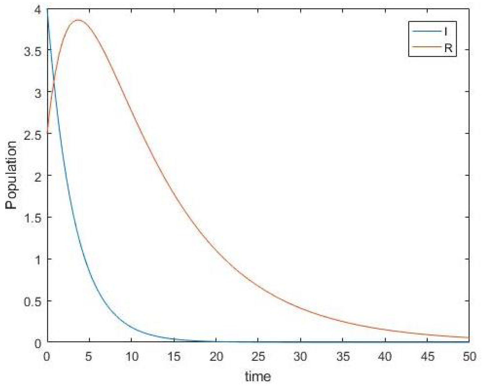
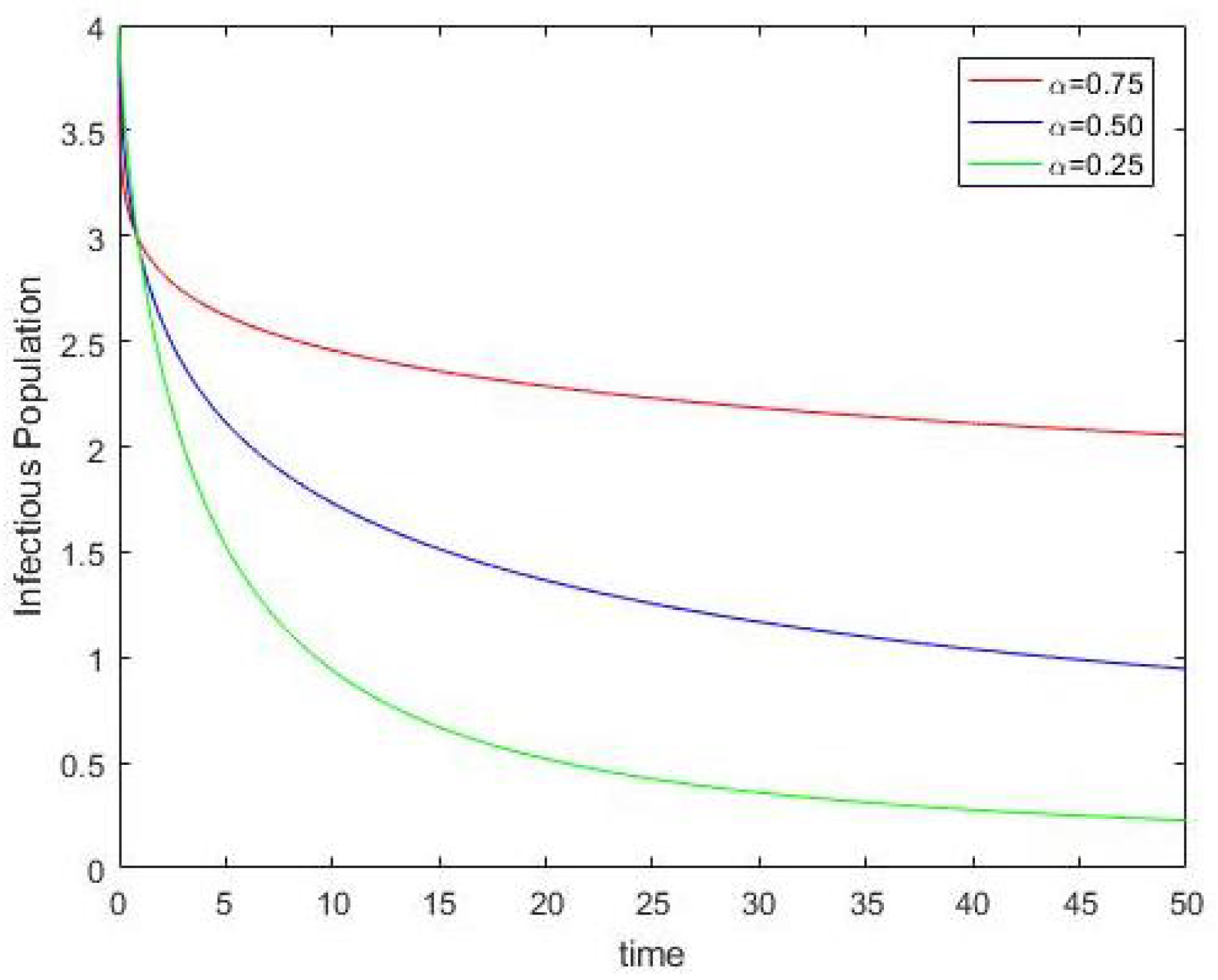
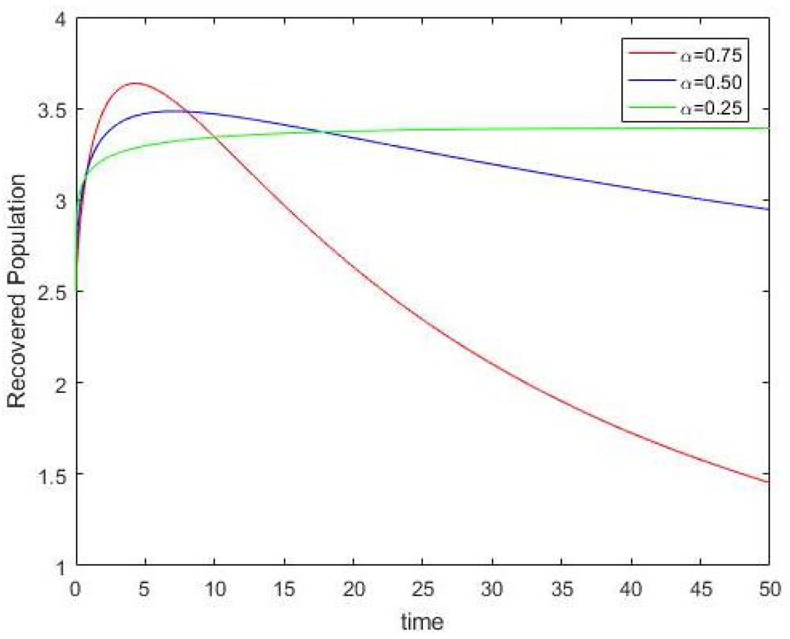
5. Numerical Simulations

In this section, the numerical simulation for $f=0.1,\mathrm{\Delta }=1,\mu =0.1;{\mu }_1=0.01,d=0.3$, Figure 1 demonstrates the dynamical behavior of an infectious and recovered population against time. Figure 2 and Figure 3 show the variation of y against t for order $\alpha =0.75,0.50,0.25$. From Figure 2, it is clear that as we decrease the index of memory $\alpha$, the infectious population decreases, and from Figure 3, it is seen that as we decrease the index of memory $\alpha$, the recovered population increases. This is also a natural fact. Hence, for $\alpha$ values, the infectious population is directly proportional to Z and the recovered population is inversely proportional to Z. Thus, ${}_0^C{D}_t^{\alpha }\left[I\left(t\right)\right]\propto Z$ and ${}_0^C{D}_t^{\alpha }\left[R\left(t\right)\right]\propto 1/Z$. This implies that ${}_0^C{D}_t^{\alpha }\left[I\left(t\right)\right]\times {}_0^C{D}_t^{\alpha }\left[R\left(t\right)\right]=$ constant. The product of $I\left(t\right)$ and $R\left(t\right)$ with the corresponding order $\alpha$ is constant. Therefore, $\alpha$ produces the change in total population enclosed by the infectious population at time $t=0$ and the recovered population at $t=5.$ The change in the population is a physical property, so $\alpha$ can be used to measure the changes in different population factors.

6. Conclusions

In this work, the fractional Lyapunov function for the fractional-order $SIR$ and $SIRS$ epidemic models was constructed. The special case of Mittag-Leffler stability, called power-law stability, was discussed. We further used Mittag-Leffler stability as well as generalized Mittag-Leffler stability criteria to find the stability of the Caputo fractional-order model $\left(12\right)$. It is also clear that ${}_0^C{D}_t^{\alpha }\dot{V}<0$ always holds, except at critical points. Therefore, system $\left(10\right)$ is a Lyapunov function for the model $\left(12\right)$. The endemic critical is globally asymptotically stable when it exists, according to the Lyapunov asymptotic stability theorem [24].

References

1. Li, Y.; Chen, Y.; Podlubny, I. Mittag-Leffler stability of fractional-order nonlinear dynamic systems. Automatica 2009, 45, 1965–1969. [Google Scholar] [CrossRef]
2. Sena, N. Cascade of fractional differential equations and generalized Mittag-Leffler stability. Int. J. Math. Model. Comput. 2020, 10, 25–35. [Google Scholar]
3. Aleksandrov, A. On the existence of a common lyapunov function for a family of nonlinear positive systems. Syst. Control Lett. 2021, 147, 1–4. [Google Scholar] [CrossRef]
4. Owoyemi, A.E.; Sulaiman, I.M.; Mamat, M.; Olowo, S.E. Stability and bifurcation analysis in a fractional-order epidemic model with sub-optimal immunity, nonlinear incidence and saturated recovery rate. Int. J. Appl. Math. 2021, 51, 515–525. [Google Scholar]
5. Goh, B.S. Management and Analysis of Biological Populations; Elsevier Science: Amsterdam, The Netherlands, 1980. [Google Scholar]
6. Agarwal, P.; Singh, R.; Rehman, A.U. Numerical solution of a hybrid mathematical model of dengue transmission with relapse and memory via Adam-Bashforth-Moulton predictor-corrector. Chaos Solit. Fractals 2021, 143, 1–20. [Google Scholar] [CrossRef]
7. Sharma, N.; Pathak, R.; Singh, R. Modeling of media impact with stability analysis and optimal solution of SEIRS epidemic model. J. Interdiscip. Math. 2019, 22, 1123–1156. [Google Scholar] [CrossRef]
8. Korobeinikov, A.; Wake, G.C. Lyapunov functions and global stability for SIR, SIRS, and SIS epidemiological models. Appl. Math. Lett. 2002, 15, 955–960. [Google Scholar] [CrossRef] [Green Version]
9. Korobeinikov, A.; Maini, P.K. A Lyapunov function and global properties for SIR and SEIR epidemiological models with nonlinear incidence. Math. Biosci. Eng. 2004, 1, 57–60. [Google Scholar] [PubMed]
10. Korobeinikov, A. Lyapunov functions and global stability for SIR and SIRS epidemiological models with the non-linear transmission. Bull. Math. Biol. 2006, 68, 615–626. [Google Scholar] [CrossRef] [PubMed] [Green Version]
11. Okuonghae, D.; Korobeinikov, A. Dynamics of tuberculosis: The effect of direct observation therapy strategy (DOTS) in Nigeria. Math. Model. Nat. Phenom. 2007, 2, 113–128. [Google Scholar] [CrossRef] [Green Version]
12. Georgescu, P.; Hsieh, Y.H. Global stability for a virus dynamics model with nonlinear incidence of infection and removal. SIAM J. Appl. Math. 2006, 67, 337–353. [Google Scholar] [CrossRef] [Green Version]
13. Arshad, S.; Sohail, A.; Javed, S. Dynamical Study of Fractional Order Tumor Model. Int. J. Comput. Methods 2015, 12, 1–12. [Google Scholar] [CrossRef]
14. Altaf, K.M.; Wahid, A.; Islam, S.; Khan, I.; Shafie, S.; Gul, T. Stability analysis of an SEIR epidemic model with non-linear saturated incidence and temporary immunity. Int. J. Adv. Appl. Math. Mech. 2015, 2, 1–14. [Google Scholar]
15. O′Regan, S.M.; Kelly, T.C.; Korobeinikov, A.; O’Callaghan, M.J.A.; Pokrovskii, A.V. Lyapunov functions for SIR and SIRS epidemic models. Appl. Math. Lett. 2010, 23, 446–448. [Google Scholar]
16. Miller, K.S.; Ross, B. An Introduction to the Fractional Calculus and Fractional Differential Equations; Wiley: New York, NY, USA, 1993. [Google Scholar]
17. Kilbas, A.A.; Srivastava, H.M.; Trujillo, J.J. Theory and Application of Fractional Differential Equations; Elsevier: Amsterdam, The Netherlands, 2006. [Google Scholar]
18. Busenberg, S.; Cooke, K. Vertically Transmitted Diseases: Models and Dynamics; Springer: Berlin, Germany, 1993. [Google Scholar]
19. Jumarie, G. Table of some basic fractional calculus formulae derived from a modified Riemann-Liouville derivative for non-differentiable functions. Appl. Math. Lett. 2009, 22, 378–385. [Google Scholar] [CrossRef]
20. Bohner, M.; Tunç, O.; Tunç, C. Qualitative analysis of caputo fractional integro–differential equations with constant delays. Comput. Appl. Math. 2021, 40, 1–17. [Google Scholar] [CrossRef]
21. Li, Y.; Chen, Y.; Podlubny, I. Stability of fractional-order nonlinear dynamic systems: Lyapunov direct method and generalized Mittag-Leffler stability. Comput. Math. Appl. 2010, 59, 1810–1821. [Google Scholar] [CrossRef] [Green Version]
22. Camacho, N.A.; Mermoud, M.A.D.; Gallegos, J.A. Lyapunov functions for fractional order systems. Commun. Nonlinear Sci. Numer. Simulat. 2014, 19, 2951–2957. [Google Scholar] [CrossRef]
23. Narendra, K.S.; Annaswamy, A.M. Stable Adaptive Systems; Dover Publications: New York, NY, USA, 2005. [Google Scholar]
24. Korobeinikov, A. Global asymptotic properties of virus dynamics models with dose-dependent parasite reproduction and virulence and non-linear incidence rate. Math. Med. Biol. 2009, 26, 225–239. [Google Scholar] [CrossRef] [PubMed]
Figure 1. Time series plot of total population.
Foundations 02 00013 g001
Figure 2. Effect of α on infectious population.
Foundations 02 00013 g002
Figure 3. Effect of α on recovered population.
Foundations 02 00013 g003
Publisher’s Note: MDPI stays neutral with regard to jurisdictional claims in published maps and institutional affiliations.