Explainable Artificial Intelligence for the Rapid Identification and Characterization of Ocean Microplastics

Abstract

Accurate identification of microplastic polymers in marine environments is essential for tracing pollution sources, understanding ecological impacts, and guiding mitigation strategies. This study presents a comprehensive, explainable-AI framework that uses Raman spectroscopy to classify pristine and weathered microplastics versus biological materials. Using a curated spectral library of 78 polymer specimens—including pristine, weathered, and biological materials—we benchmark seven supervised machine learning models (Decision Trees, Random Forest, k-Nearest Neighbours, Neural Networks, LightGBM, XGBoost and Support Vector Machines) without and with Principal Component Analysis for binary classification. Although k-Nearest Neighbours and Support Vector Machines achieved the highest single metric accuracy (82.5%), k NN also recorded the highest recall both with and without PCA, thereby offering the most balanced overall performance. To enhance interpretability, we employed SHapley Additive exPlanations, which revealed chemically meaningful spectral regions (notably near 700 cm⁻¹ and 1080 cm⁻¹) as critical to model predictions. Notably, models trained without Principal Component Analysis provided clearer feature attributions, suggesting improved interpretability in raw spectral space. This pipeline surpasses traditional spectral matching techniques and also delivers transparent insights into classification logic. Our findings can support scalable, real-time deployment of AI-based tools for oceanic microplastic monitoring and environmental policy development.

1. Introduction

1.1. Preamble

In recent years, plastic pollution has emerged as a global environmental and public health concern. With plastic production exceeding 400 million tons annually, the omnipresence of synthetic polymers across terrestrial and aquatic ecosystems has triggered what some now refer to as the ‘Plastic Age’ [1,2]. Historical data (Figure 1) show an exponential increase in production of plastics, starting from near zero in 1950 to over 450 million tonnes annually by 2020. The widespread spread of plastic waste presents a serious risk to ecosystems and human well-being. Of particular concern is the proliferation of microplastics (MPs)—plastic particles typically smaller than 5 mm—which have infiltrated marine environments at an alarming scale [3,4,5]. MPs originate from both primary sources (such as industrial abrasives and microbeads) and secondary sources, including the fragmentation of larger plastic debris through photochemical and mechanical weathering [6,7].

Marine environments are considered to be the ones most severely affected by microplastic pollution among all ecosystems [5,8]. Furthermore, modelling studies [9] have suggested that over 5.25 trillion plastic particles, weighing approximately 268,940 tons, are currently floating in the world’s oceans. Deep-sea MPs are primarily the result of maritime activities, including shipping (accidental spills, improper waste disposal), offshore platform operations, and commercial and recreational fishing. In contrast, coastal MPs come predominantly from land sources, entering the ocean through discharge of wastewater, river transport, surface runoff, and atmospheric deposition [6,10].

The ubiquity of microplastics in oceanic systems poses a multifaceted threat, not only to marine life but also to human health through a concept known as One Health, which recognizes the interconnection of environmental, animal and human health [2,6,8,11]. Microplastics can be ingested by plankton and small fish, accumulate in larger predators through trophic transfer, and ultimately enter the human food chain via seafood consumption [12]. These particles can act as vectors for toxic additives or adsorbed environmental pollutants, compounding their potential to disrupt endocrine, immune, and metabolic functions in exposed organisms—including humans [2,6,11].

At the molecular level, microplastics are made up of various synthetic polymers, each exhibiting distinct physicochemical properties and environmental behaviour [2]. Accurate identification of these polymer types is, therefore, critical, in order to trace their sources and understand their environmental persistence, and also to assess their toxicological implications across the biosphere. Robust polymer identification underpins risk assessments, informs regulatory policies, and supports mitigation strategies aligned with the principles of Public and One Health [2,6].

1.2. Motivation and Contribution

Accurate distinction of anthropogenic microplastics from naturally occurring biopolymers remains a persistent obstacle in environmental monitoring and risk assessment [13]. Although the open-access Raman spectral library compiled by Miller [14] can provide a valuable foundation—covering pristine and weathered consumer, industrial, and fishing gear plastics, as well as commonly misidentified biological materials, e.g., cellulose, keratin, and calcium carbonate matrices—it remains a static resource on its own. Converting that reference archive into a practical, real time decision support system demands an analytical engine that can both classify spectra reliably under variable field conditions and reveal the rationale behind each prediction for scientific audit and regulatory scrutiny.

The present study addresses this need, by developing an explainable artificial intelligence (XAI) framework capable of distinguishing between biological and anthropogenic polymers based on Raman spectral features. Utilizing supervised machine learning models in conjunction with SHAP (SHapley Additive exPlanations), transparent and interpretable insights into the decision-making process of the classifier are provided. This ensures model accountability and also aids in identifying the most informative spectral regions associated with polymer type. By integrating explainability into the classification pipeline, our approach supports the development of robust, real-time microplastic monitoring systems with the potential for scalable deployment in environmental surveillance and regulatory contexts.

2. Related Work

By the end of the year 2024, over 1600 studies will have been published internationally on microplastic detection, However, less than 100 among these have explored the application of artificial intelligence (AI) in this context. Compared to other scientific domains, the integration of AI in microplastic research remains relatively underdeveloped. This highlights the novelty and timeliness of the present work, which represents a further step toward bridging this gap by using AI-driven approaches for microplastic classification and analysis [15]. Yang et al. [16] have presented a comprehensive review of atmospheric microplastics, addressing their sources, distribution, environmental behaviour, and toxicological effects. The study highlights the underutilized role of machine learning in advancing atmospheric MPs research, particularly in source apportionment, spatiotemporal analysis, and toxicity prediction. Hu et al. [17] have presented an extensive review of machine learning methodologies applied to the prediction of MPs across a range of analytical tasks. The study provides an in-depth discussion on data sources, preprocessing strategies, core algorithmic frameworks, and inherent limitations of the employed techniques. Furthermore, it critically evaluates the current constraints of machine learning in MP-related analyses and outlines potential directions for future research. Hoppener et al. [18] propose a novel proof-of-concept methodology that combines cathodoluminescence (CL) with scanning electron microscopy (SEM) and machine learning to classify microplastics and nanoplastics (MNPs). By generating a spectral database from over 100 plastic samples and training neural network classifiers, the authors have achieved high classification accuracy (97%), even distinguishing difficult materials like black plastics. This method can enhance nanoscale detection and will expand the toolbox for precise microplastic identification. Another study has combined Raman spectroscopy with a sparse autoencoder (SAE) and softmax classifier framework to enable the rapid and accurate identification of six common microplastic types (PET, PVC, PP, PS, PC, PE) across five types of water environments [19]. The method can achieve a classification accuracy of 99.1%, outperforming traditional SVM and BP neural network methods. Moreover, the application of Neural Networks for identifying microplastics in hyperspectral images has also been assessed [20]. The goal in that study was to assess the feasibility of hyperspectral imaging as a detection tool in environmental monitoring of microplastic pollution. Weber et al. [21] develop a deep learning-based framework using µ-Raman spectroscopy to automate microplastic detection in environmental samples. Using over 64,000 spectra, these authors have proposed a human–machine teaming method that significantly reduces analysis time. Their best model achieved precision and recall rates over 97% and 99%, respectively. The study demonstrates how ML can significantly enhance the efficiency and scalability of microplastic pollution analysis. In another study [22], the authors used the k-Nearest Neighbours machine learning algorithm to classify thousands of FTIR spectra collected from microplastics in the Mediterranean Sea. Their algorithm achieved high accuracy when benchmarked against expert annotation, with fewer than 10% discrepancies, most of which were easily correctable.

Liu et al. [23] used six machine learning algorithms to predict the cytotoxicity of five common microplastics on human lung cells. The extreme gradient boosting model exhibited the highest predictive power (R2 = 0.93). SHAP and other feature importance methods consistently identified particle size as the most influential feature. The models have offered a cost-effective tool for assessing health risks associated with microplastic exposure. The work of Yan et al. [24] has introduced an ensemble machine learning framework for microplastic identification using FTIR spectroscopy data. This model outperforms single ML models by improving classification accuracy and robustness, particularly on imbalanced and noisy datasets, making it a promising solution for automated microplastic identification in complex samples. Qiu et al. [25] gathered 475 sorption data points from existing literature and introduced an innovative machine learning model incorporating a poly-parameter linear free energy relationship. Among the algorithms evaluated, a hybrid model combining a genetic algorithm with Support Vector Machines showed the highest predictive accuracy (R2 = 0.93, RMSE = 0.07).

3. Materials and Methods

3.1. Dataset

The current dataset [14,26] consists of a total of 78 polymer specimens, which were scanned using 532 nm and 785 nm Raman systems. Samples were mounted on glass slides using ethylene-vinyl acetate resin. Spectra were preprocessed using polynomial fitting, standard normal variate (SNV) normalization, and rescaling to allow comparability across samples. Pearson correlation coefficients and hierarchical clustering were originally used in the source dataset to assess intra- and inter-polymer variation. A matching script in R is provided for reproducibility. Also, the dataset includes raw and processed spectra for pristine, weathered, and biological polymer samples. Validation of the spectral assignments was performed in the original publication using both internal comparison and a proprietary commercial Raman library. The accuracy of the reference library was demonstrated through a case study identifying a weathered strawberry basket as polypropylene.

In this study, a representative subset of 78 spectra (1 per specimen) [26] was used to ensure balanced and interpretable classification. The dataset covers three categories: (a) pristine anthropogenic polymers newly sourced from manufacturers (n = 39), (b) weathered anthropogenic polymers collected from consumer waste, beachcast debris, agricultural runoff, and fishery by-catch (n = 22), and (c) biological polymers representing diverse marine taxa, trophic levels, and tissues (n = 17). This design provides chemically diverse spectra for robust model training and validation while maintaining class balance [26].

3.2. Data Processing

The Raman spectra used in this study were sourced from the open-access spectral reference library [14], which includes high-quality Raman spectra from 78 specimens categorized into pristine anthropogenic polymers, weathered plastics, and biological materials found in marine environments. To investigate the effect of spectral resolution on model performance, two spectral variants of the dataset were employed:

• Restricted Range: 200 to 1700 cm⁻¹, covering the classical fingerprint region rich in polymer-specific vibrations and
• Full Range: 200 to 3400 cm⁻¹, including higher wavenumber regions capturing C-H, O-H, and N-H stretching bands relevant for broader material characterization.

All spectra were pre-processed following the methodology of the original dataset using R-based scripts: a 15-point median filter was applied to remove noise, followed by a 7th-order polynomial baseline correction. Standard Normal Variate (SNV) normalization and min–max rescaling (0–1) were then used to ensure consistency across spectra.

3.3. Methodological Procedure

The methodological pipeline used in this study is outlined in Figure 2. The procedure began with an open-access spectral reference library comprising 78 specimens of plastic and biological materials. The spectral data underwent several preprocessing steps to enhance quality and comparability. These included a 15-point median filter to reduce random noise, a 7th-order polynomial baseline correction to eliminate fluorescence effects, Standard Normal Variate (SNV) normalization to correct for scattering differences, and min–max rescaling to scale the intensity values between 0 and 1. Following preprocessing and in order to evaluate model generalizability, a repeated random sub-sampling strategy was employed.

Fifty independent train–test splits were generated using an 80:20 ratio, each based on a different random seed. Care was taken to ensure stratified representation across the two main polymer categories (pristine and weathered in one category and biological in the second category) within each split. Each model was trained and evaluated on both spectral variants (200–1700 cm⁻¹ and 200–3400 cm⁻¹) using identical splits to allow direct performance comparisons. In the first, a broad comparison of multiple machine learning algorithms (Decision Trees, Random Forest, k-Nearest Neighbours, Neural Networks, Support Vector Machines, LightGBM, XGBoost) was conducted. In the second, a focused comparison was carried out between LightGBM and Support Vector Machines and under consistent conditions. Model selection was based on standard performance metrics, which included accuracy, recall, precision, and F1-score.

In order to interpret correctly model behaviour and to identify influential spectral features, SHapley Additive exPlanations (SHAP) were applied to the best-performing models. The resulting insights were further contextualized through XAI visualization, enabling a spatially informed representation of EMF exposure patterns derived from spectral classification outputs.

3.4. Machine Learning Tools Employed in This Work

3.4.1. Decision Trees

Decision Trees were employed as baseline models due to their effectiveness in handling both categorical and continuous variables. Their hierarchical structure made the tool ideal for capturing distinct patterns in Raman spectral data. Pruning was applied, in order to enhance generalization and to reduce overfitting.

3.4.2. Random Forest

Random Forest, an ensemble composed of numerous Decision Trees, can provide greater predictive accuracy and stability. Each tree was trained on bootstrapped subsets, effectively reducing variance and mitigating overfitting. The ensemble structure would allow for capturing intricate feature interactions and robustness against noisy Raman spectra.

3.4.3. K-Nearest Neighbours

The k-Nearest Neighbours (k-NN) algorithm utilized local spectral similarity for prediction, effectively identifying meaningful local patterns within the Raman dataset. Despite sensitivity to feature scaling, k-NN would maintain competitive performance, emphasizing the local structure of spectral data.

3.4.4. Neural Networks

Feedforward Neural Networks were used to model non-linear relationships between spectral inputs and classification labels. Training employed backpropagation, with regularization methods, e.g., dropout and early stopping, included to prevent overfitting. Despite the tool’s requirement for substantial data in order to achieve optimal performance, Neural Networks can capture effectively complex interactions among spectral features.

3.4.5. Support Vector Machines

Support Vector Machine is a supervised learning algorithm that addresses the challenge of sample efficiency by identifying decision boundaries (termed hyperplanes), which separate data points correctly and also maximize the margin between the boundary and the closest training examples. By focusing on large-margin separation, the tool can achieve strong generalization with fewer training samples, even in high-dimensional or infinite-dimensional feature spaces.

3.4.6. LightGBM

LightGBM was selected for its computational efficiency and strong predictive performance on structured spectral data. Using histogram-based gradient boosting with leaf-wise tree growth, the method provided rapid training and effectively handled complex spectral feature interactions.

3.4.7. XGBoost

XGBoost, known for its robustness in handling high-dimensional datasets and built-in regularization, effectively modelled the non-linear structure inherent to Raman spectra. The tool can gracefully manage noisy or incomplete spectral data, achieving reliable and precise predictions.

3.4.8. Motivation for Applying Principal Component Analysis

Principal Component Analysis (PCA) was applied due to the densely sampled and highly correlated nature of Raman spectral data, which typically would increase dimensionality with no proportional gain in discriminative power. PCA transformed correlated spectral features into a smaller set of uncorrelated components that encapsulate the dominant variance [27].

Projecting spectral data onto a reduced-dimensional space via PCA improved numerical stability, reduced noise, and mitigated overfitting risks, especially relevant in limited or imbalanced datasets [28]. Algorithms such as k-Nearest Neighbours and Neural Networks benefit substantially from lower-dimensional representations, alleviating issues associated with high dimensionality [29]. Thus, PCA served effectively to maintain critical biochemical information, while enhancing computational efficiency and interpretability [30].

Table 1. Machine learning tools and relevant hyperparameters employed in the study.

Machine Learning Tool	Hyperparameters
Decision Tree	Criterion: gini, entropy	Maximum depth: 5, 10
	Minimum samples split: 2, 50	Minimum samples leaf: 1, 10
Random Forest	Number of trees: 50, 100, 200	Criterion: gini, entropy
	Maximum depth: 10
k-Nearest Neighbours	Number of neighbours (k): 5, 25, 40	Distance metric (p): 1, 1.5, 2, 3
	Weighing: uniform, distance
Neural Networks	Hidden layer size: 5, 10, 20	Learning rate: 0.01, 0.1
	Activation: ReLU
Support Vector Machines	Kernel: linear, RBF	Regularization (C): 0.1, 1, 10
LightGBM	Number of leaves: 31, 100	Number of estimators: 100, 300, 500
	Learning rate: 0.01, 0.1	Maximum depth: 5, 20
XGBoost	Regularization (C): 1, 5	Number of estimators: 300, 500
	Learning rate: 0.05, 0.1	Maximum depth: 5, 10

presents a comparative overview of the machine learning tools employed in the current work. The table outlines the specific hyperparameters explored for each model. The relevant hyperparameter ranges are summarized, reflecting the tuning process that aimed at optimizing classification accuracy, precision, recall, and F1-score. This structured overview provides a concise reference for replicating or extending the experimental setup, emphasizing the systematic approach taken in model selection and optimization.

3.5. Model Interpretability

In order to achieve interpretability, Shapley Additive Explanations (SHAP), grounded in cooperative game theory, were employed to quantify the contribution of individual features. SHAP provided both global and local insights, globally highlighting the most influential Raman spectral regions and locally elucidating individual prediction behaviours. Visualization tools, such as SHAP summary plots and dependence plots, illustrated the relationships between spectral features and predictive outcomes. These analyses clarified the behaviour of complex models, improving transparency and interpretability in Raman-based classification tasks. To preserve chemical interpretability, the classifier for the SHAP was trained directly on the raw absorbance values at each recorded wavenumber, foregoing any principal component analysis (PCA) preprocessing. Retaining the native spectral variables maintains a one-to-one correspondence between each input feature and a specific vibrational frequency. Consequently, post hoc explainable-AI methods—here SHAP value analysis and permutation feature importance—can assign predictive weight unambiguously to individual wavenumbers, revealing which vibrational modes (and, by extension, which biochemical constituents) drive class separation. On this basis, all results reported herein employ the raw spectral matrix, prioritizing transparency, ease of biological validation, and translational credibility over negligible accuracy improvements.

4. Results

For each ML tool, the four hyperparameter settings that achieved the highest mean performance are reported herein. For each model, the top four configurations are shown with their primary metric (e.g., mean accuracy, mean recall, mean precision and mean F1-score). That way, a concise comparison of the effects of tuning parameters (e.g., learning rate, number of estimators (or leaves), regularization strength, kernel choice, and tree depth) could be made, as well as highlighting the most promising configurations for further analysis. In the below figures, each cluster of bars shows four metrics: accuracy, precision, recall, and F1-score, the tables list the mean score of each model’s optimal hyper-parameter configuration.

4.1. Evaluation of the Various Models Without Application of PCA

4.1.1. Decision Trees

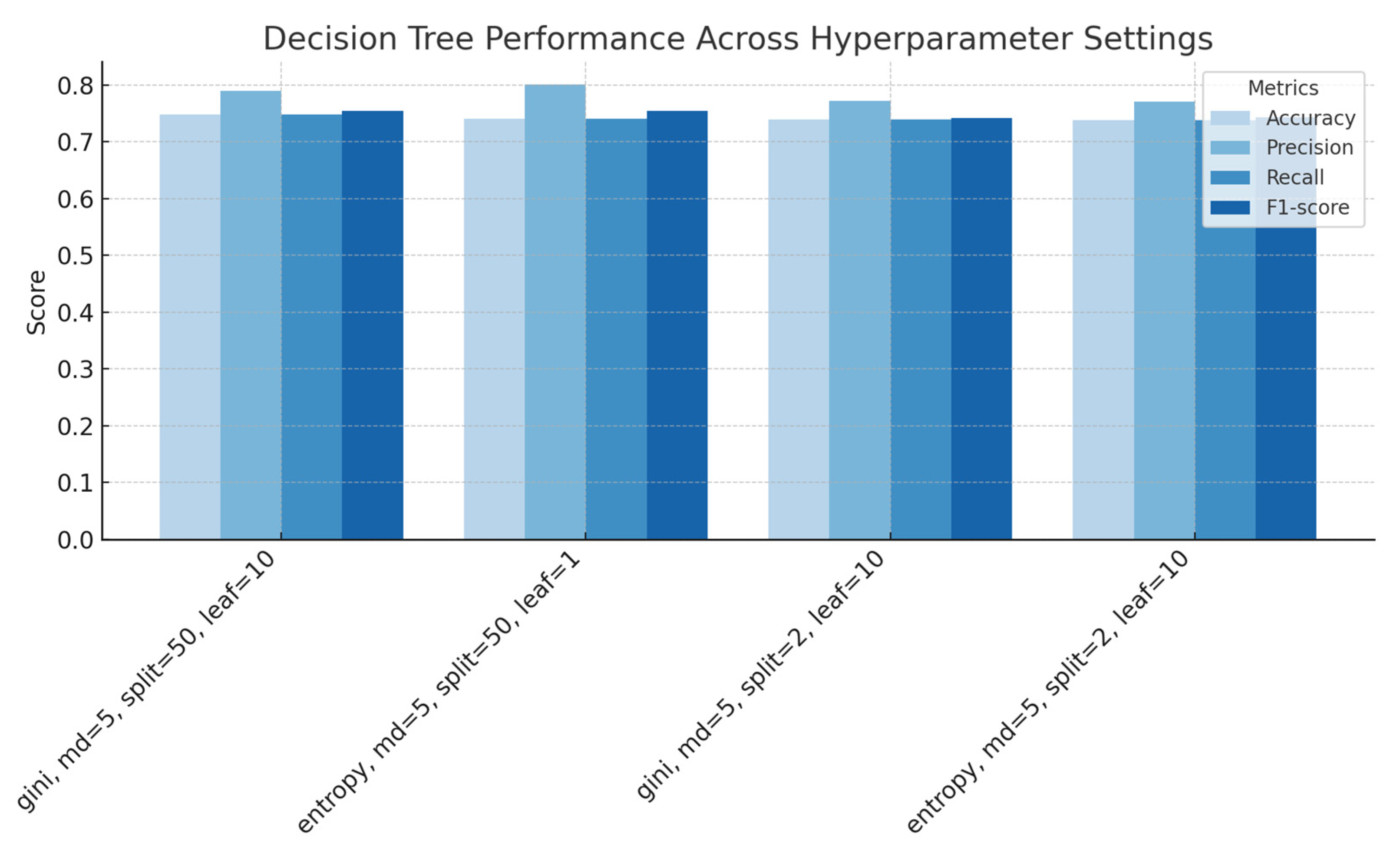
Figure 3 compares the performance of Decision Trees models under four hyperparameter settings: Gini impurity versus. entropy, minimum samples split of 50 versus 2 and minimum samples leaf of 10 versus 1 (all with max depth: 5).

The highest precision (0.802) was observed for the entropy criterion with a split of 50 and leaf size of 1, albeit with a modest reduction in accuracy (0.741). Conversely, the Gini criterion with split = 50 and leaf = 10 yielded the highest accuracy (0.749) but slightly lower precision (0.790). Reducing the minimum samples split to two led to marginal declines across metrics, indicating that larger split thresholds and leaf sizes helped to mitigate overfitting while maintaining balanced classification performance. Hence, the optimal model of Decision Tree classifier was the one using the Gini impurity criterion, with maximum depth = 5, minimum samples split = 50, and minimum samples leaf = 10 (

Table 2. Performance metrics for Decision Trees with Gini Criterion.

Metric	Mean	Standard Deviation	95% Lower Confidence Interval	95% Upper Confidence Interval
Accuracy	0.749	0.107	0.719	0.778
Precision	0.790	0.105	0.761	0.819
Recall	0.749	0.107	0.719	0.778
F1-score	0.755	0.099	0.728	0.782

).

4.1.2. Random Forest

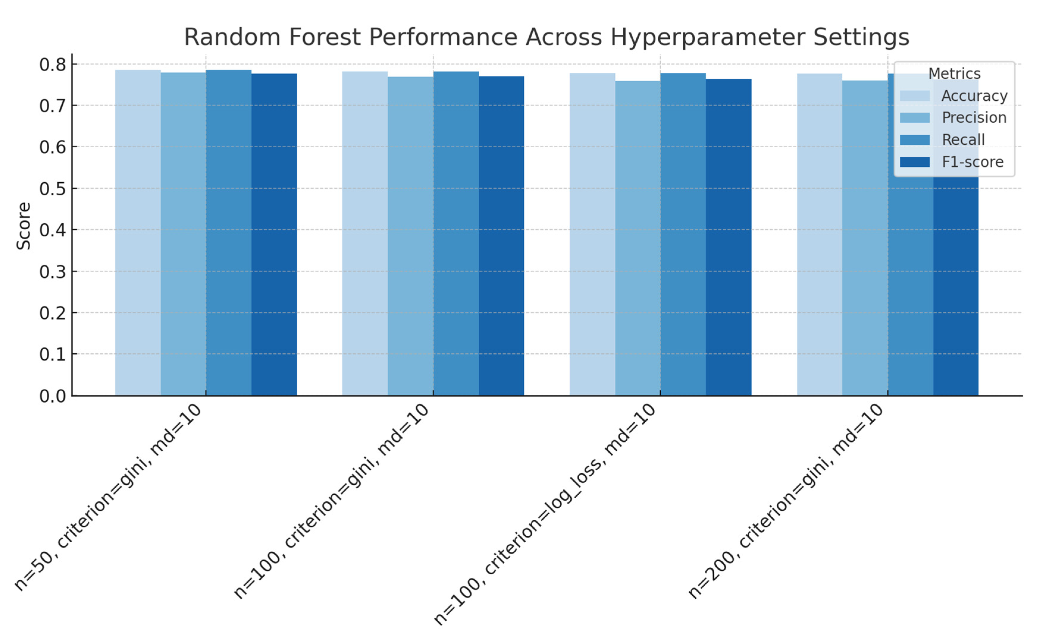
Figure 4 compares the performance of Random Forest models under four hyperparameter settings: Gini impurity versus. entropy, minimum samples split of 50 versus 2 and minimum samples leaf of 10 versus 1 (all with max depth: 5).

Accuracy and recall peaked at 0.785 for the smallest forest (50 trees, Gini), where precision and F1-score also reached their highest values (0.779 and 0.776, respectively). An increase in the forest to 100 trees with Gini slightly lowered all metrics, whilst switching to log-loss further reduced performance (accuracy 0.778, F1-score 0.763). Expanding the forest to 200 trees yielded marginal additional declines, suggesting that neither a larger ensemble, nor an alternative split criterion substantially benefited this classification task and that small forests might suffice (

Table 3. Performance metrics for Random Forest with Gini Criterion.

Metric	Mean	Standard Deviation	95% Lower Confidence Interval	95% Upper Confidence Interval
Accuracy	0.785	0.093	0.756	0.807
Precision	0.779	0.108	0.739	0.799
Recall	0.785	0.093	0.756	0.807
F1-score	0.776	0.094	0.744	0.796

). Overall, the Random Forest tool showed solid predictive performance, with consistent precision and recall across the evaluation folds.

4.1.3. K-Nearest Neighbours

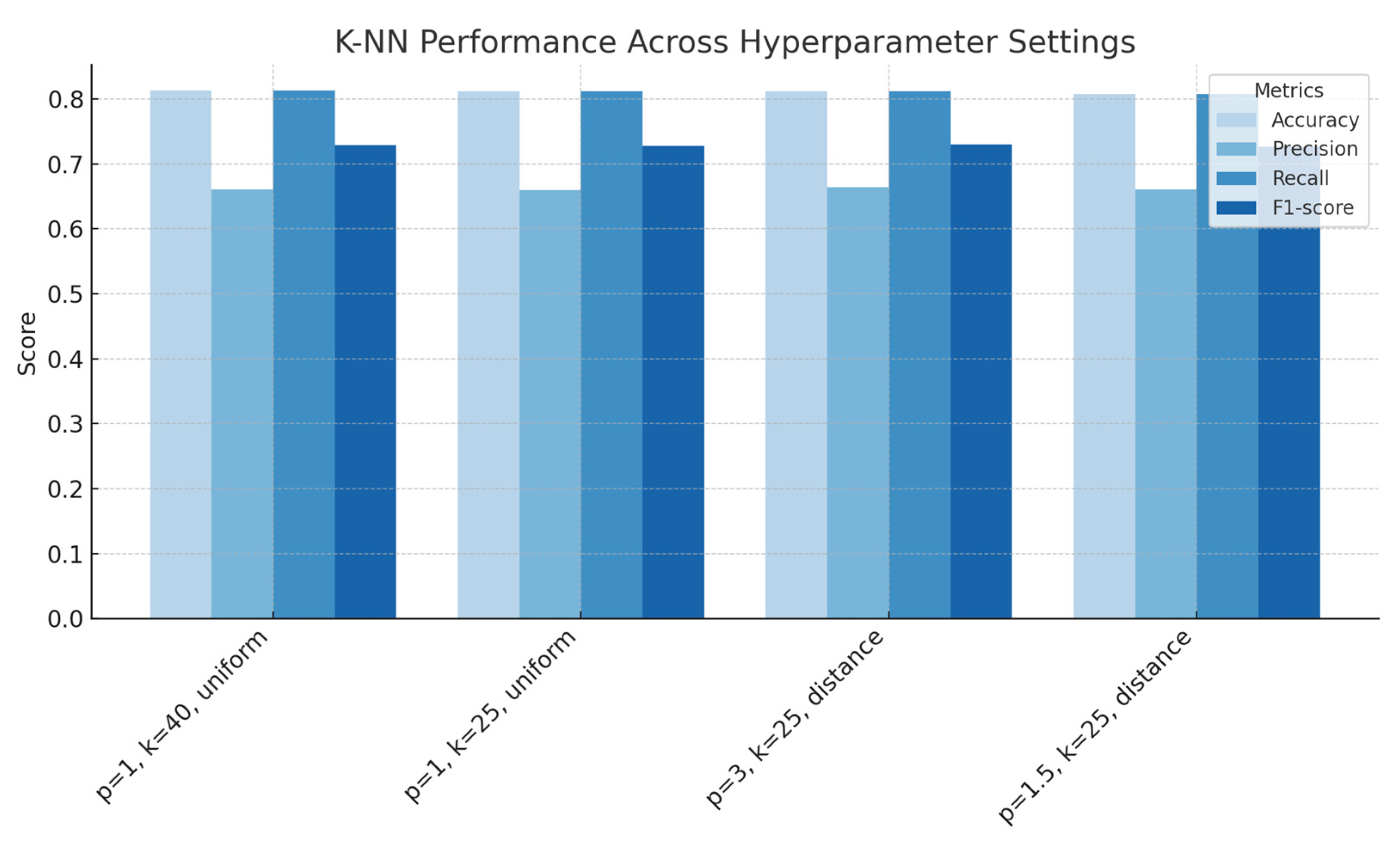
Figure 5 depicts the performance of k-NN classifiers under four hyperparameter settings: [k = 40, p = 1, uniform weights], [k = 25, p = 1, uniform weights], [k = 25, p = 3, distance weights], and [k = 25, p = 1.5, distance weights].

The highest accuracy and recall (0.813) were achieved with p = 1, k = 40, uniform weights, though precision was lower (0.660), yielding an F1-score of 0.728. Reducing k to 25, slightly decreased accuracy and recall, while switching to distance-based weights with p = 3 partly recovered precision (0.664) and F1-score (0.730). Lowering the norm to p = 1.5 with distance weights resulted in the lowest performance overall, suggesting that neighbour count and distance weighing jointly influenced the balance between precision and recall in k-NN classification (

Table 4. Performance metrics for k-Nearest Neighbours.

Metric	Mean	Standard Deviation	95% Lower Confidence Interval	95% Upper Confidence Interval
Accuracy	0.813	<0.001	0.813	0.813
Precision	0.660	<0.001	0.660	0.660
Recall	0.813	<0.001	0.813	0.813
F1-score	0.728	<0.001	0.728	0.728

).

4.1.4. Neural Networks

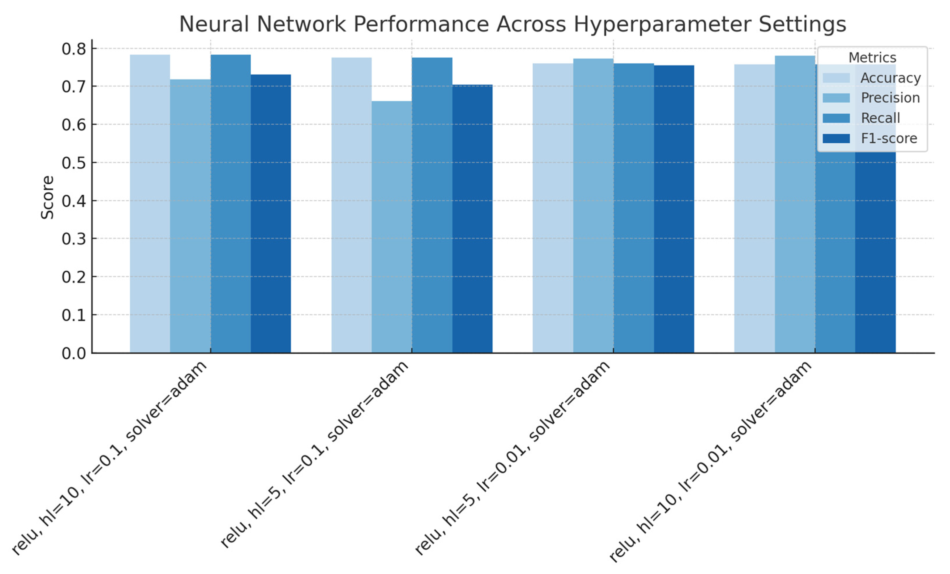
Figure 6 depicts the performance of neural network classifiers (using ReLU activation and Adam solver) under four configurations: hidden layer size (n = 10 or 5) and initial learning rate (0.1 or 0.01).

The best overall accuracy and recall (0.784) was seen with 10 neurons in the hidden layer and a high learning rate (0.1), though precision was lower (0.718), which resulted in an F1-score of 0.731. Halving the layer size reduced accuracy and recall slightly, with precision reduced to 0.661. Decrease in the learning rate to 0.01 improved precision (to 0.7810) but at the cost of a reduced accuracy (0.758) and some modest F1 change. The results illustrate the trade-off between learning rate and network capacity in balancing the precision–recall performance (

Table 5. Performance metrics for Neural Networks.

Metric	Mean	Standard Deviation	95% Lower Confidence Interval	95% Upper Confidence Interval
Accuracy	0.784	0.107	0.754	0.814
Precision	0.718	0.095	0.692	0.744
Recall	0.784	0.107	0.754	0.814
F1-score	0.731	0.096	0.704	0.757

).

4.1.5. Support Vector Machines

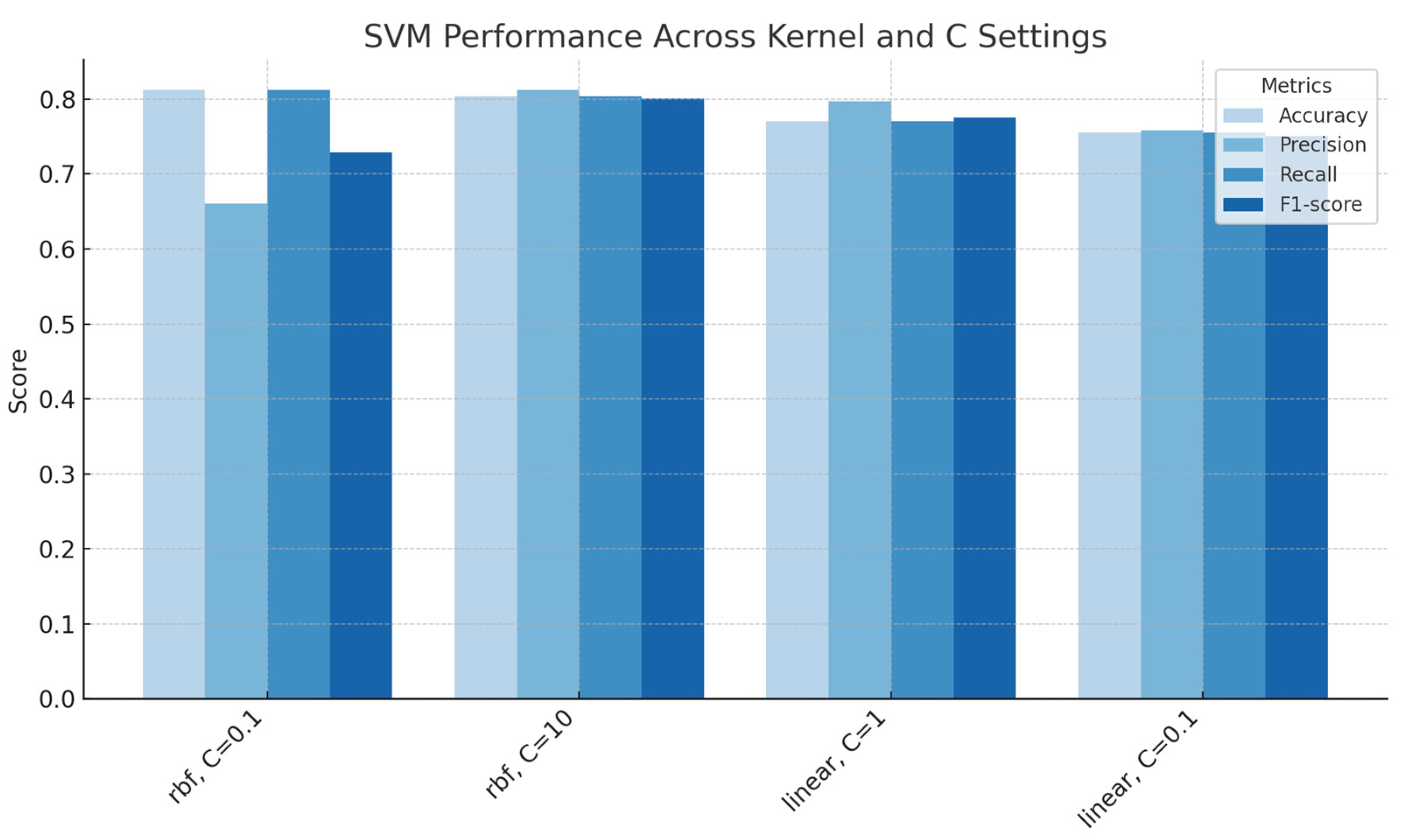
Figure 7 compares the performance of Support Vector Machine models with different kernel functions (RBF and linear) and regularization strengths (C).

The RBF kernel at C = 0.1 achieved the highest precision and recall (0.813), but showed lower precision (0.660), resulting in an intermediate F1 score (0.728). Increasing C to 10 balanced precision (0.812) and recall (0.804), producing a higher F1-score (0.801). For the linear kernel, performance dropped slightly, with the best results at C = 1 (accuracy and recall: 0.770, precision: 0.800, F1-score: 0.775), and further declined at C = 0.1. Overall, these suggested that both kernel choice and regularization parameter significantly influenced precision–recall trade-offs in Support Vector Machines classification. Therefore, the optimal and the most stable model of Support Vector Machines classifier is the one with radial basis function (RBF) kernel with a regularization parameter C = 10 (

Table 6. Performance metrics for Support Vector Machines with RBF Kernel (C = 0.1).

Metric	Mean	Standard Deviation	95% Lower Confidence Interval	95% Upper Confidence Interval
Accuracy	0.812	0.000	0.813	0.813
Precision	0.812	0.000	0.660	0.660
Recall	0.804	0.000	0.813	0.813
F1-score	0.801	<0.001	0.728	0.728

).

4.1.6. LightGBM

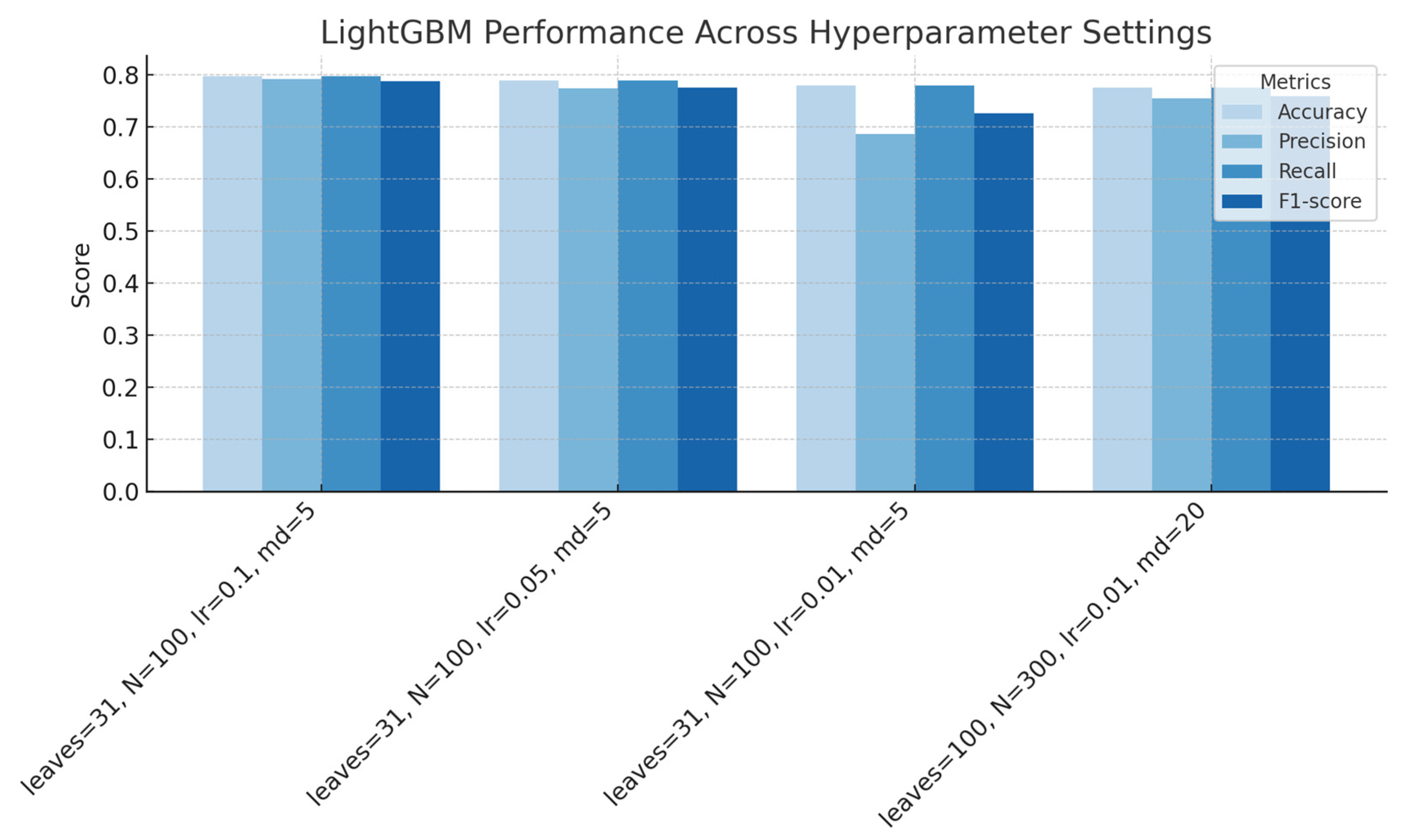
Figure 8 illustrates the performance of LightGBM models under four different hyperparameter configurations. The highest overall performance was achieved with 31 leaves, 100 estimators, a learning rate of 0.1, and maximum depth of 5 (accuracy: 0.798, recall: 0.798, precision: 0.792, F1-score: 0.788).

Decrease in the learning rate to 0.05 and 0.01 at the same leaf and estimator settings resulted to gradual declines across all metrics, most notably precision (reduced to 0.686 with learning rate at 0.01). Increase in the number of leaves to 100 and the number of estimators to 300 (with learning rate = 0.01 and maximum depth = 20) further reduced the performance, which might indicate that both the learning rate and the complexity of the tree significantly affected the efficacy of the model. Hence, the optimal configuration of the LightGBM classifier was with number of leaves = 31, number of estimators = 100, learning rate = 0.1, and maximum depth = 5 (

Table 7. Performance metrics for LightGBM configuration.

Metric	Mean	Standard Deviation	95% Lower Confidence Interval	95% Upper Confidence Interval
Accuracy	0.798	0.091	0.772	0.823
Precision	0.792	0.110	0.761	0.822
Recall	0.798	0.091	0.772	0.823
F1-score	0.788	0.094	0.762	0.814

).

4.1.7. XGBoost

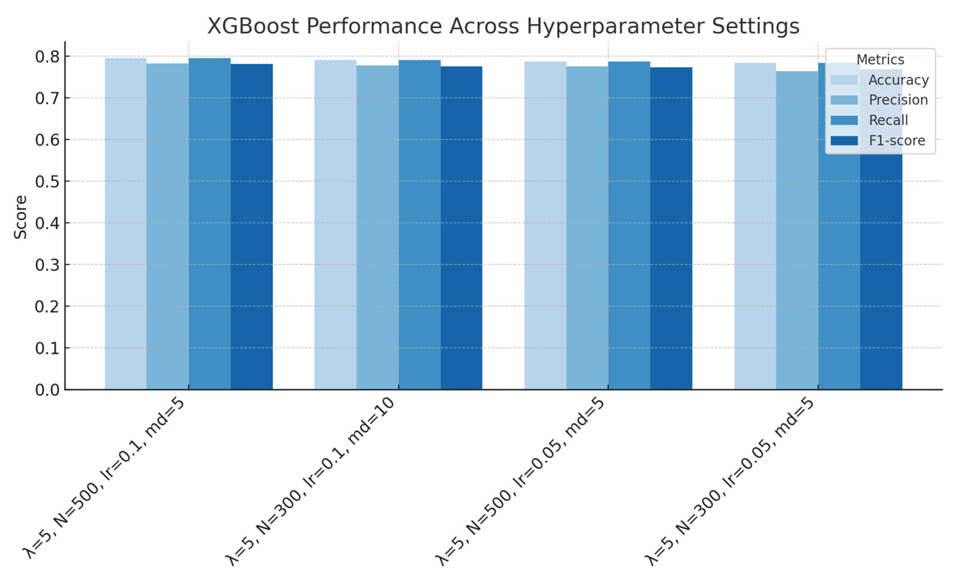
Figure 9 compares XGBoost models with no PCA performed under the following four configurations: (a) λ = 5, N = 500, lr = 0.1, md = 5→274 (where md = max_depth), (b) λ = 5, N = 300, lr = 0.1, md = 10, (c) λ = 5, N = 500, lr = 0.05, md = 5 and (d) λ = 5, N = 300, lr = 0.05, md = 5.

The highest accuracy (0.795), recall (0.795), precision (0.782) and F1-score (0.781) occurred with λ = 5, N = 500, lr = 0.1 and maximum depth = 5. A reduction in the number of estimators or learning rate gradually decreased performance, indicating that ensemble size and learning rate were critical factors in capturing model effectiveness without dimensionality reduction. Hence, the optimal configuration of the XGBoost classifier was with λ = 5, N = 500, learning_rate = 0.1, and max_depth = 5 (

Table 8. Performance metrics for XGBoost Configuration.

Metric	Mean	Standard Deviation	95% Lower Confidence Interval	95% Upper Confidence Interval
Accuracy	0.795	0.096	0.763	0.817
Precision	0.782	0.112	0.747	0.809
Recall	0.790	0.096	0.763	0.817
F1-score	0.781	0.095	0.749	0.802

). The model showed 286 stable predictive behaviour with balanced precision and recall scores.

4.1.8. Comparison Between Models

In

Table 9. Comparison of performance metrics for seven machine learning tools without PCA.

Metric	Accuracy	Precision	Recall	F1-Score
Decision Tree	0.749	0.790	0.749	0.755
Random Forest	0.785	0.779	0.785	0.776
k-Nearest Neighbours	0.813	0.660	0.813	0.728
Neural Networks	0.784	0.718	0.784	0.731
Support Vector Machines	0.812	0.812	0.804	0.801
LightGBM	0.798	0.792	0.798	0.788
XGBoost	0.795	0.782	0.790	0.781

, a summary comparison of the performance of the seven machine learning tools employed and the models evaluated is shown. This is based on the mean accuracy, precision, recall, and F1-score for each of the seven tools. Among the tools, k-Nearest Neighbours and Support Vector Machines achieved the highest accuracy (0.812 and 0.813), showing strong correct classification capability. In terms of F1-score, which balances precision and recall, the Support Vector Machines outperformed all other tools with the highest F1-score (0.801), indicating its robust performance in handling class imbalances. Overall, the k-Nearest Neighbour and the Support Vector Machines achieved the top accuracy, but LightGBM delivered the best balance between precision and recall. This made it the most effective model in terms of overall classification performance.

4.2. Evaluation of the Various Models with Application of PCA

4.2.1. Decision Trees

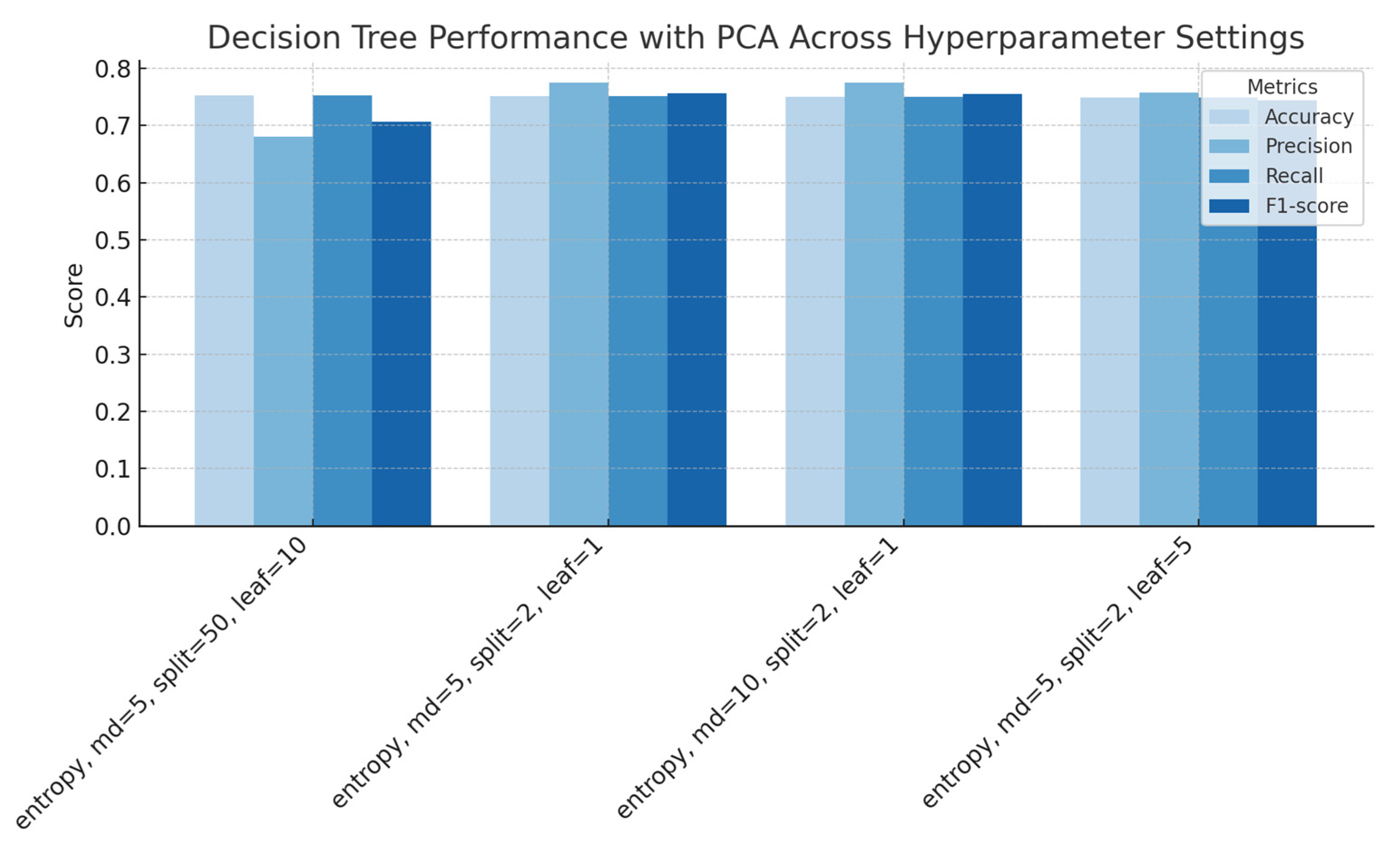
Figure 10 illustrates the performance of Decision Trees classifiers on PCA-transformed data under four hyperparameter configurations: (a) entropy criterion, max depth = 5, min. samples split = 50, min. samples leaf = 10, (b) entropy criterion, max depth = 5, min. samples split = 2, min. samples leaf = 1, (c) entropy criterion, max depth = 10, min. samples split = 2, min. samples leaf = 1, (d) entropy criterion, max depth = 5, min. samples split = 2, min. samples leaf = 5.

The highest accuracy and recall (0.753) occurred at the configuration with split = 50 and leaf = 10, while the highest precision (0.775) and F1-score (0.756) were achieved at split = 2, leaf = 1 with depth = 5. Increasing the maximum depth to 10, yielded marginal declines, indicating that lower complexity trees on PCA-reduced features could balance precision and recall effectively.

Table 10. Performance metrics for Decision Trees with PCA.

Metric	Mean	Standard Deviation	95% Lower Confidence Interval	95% Upper Confidence Interval
Accuracy	0.753	0.091	0.727	0.778
Precision	0.681	0.051	0.667	0.695
Recall	0.753	0.091	0.727	0.778
F1-score	0.706	0.051	0.692	0.720

presents the optimal performance, with accuracy, precision, recall, and F1-score.

4.2.2. Random Forest

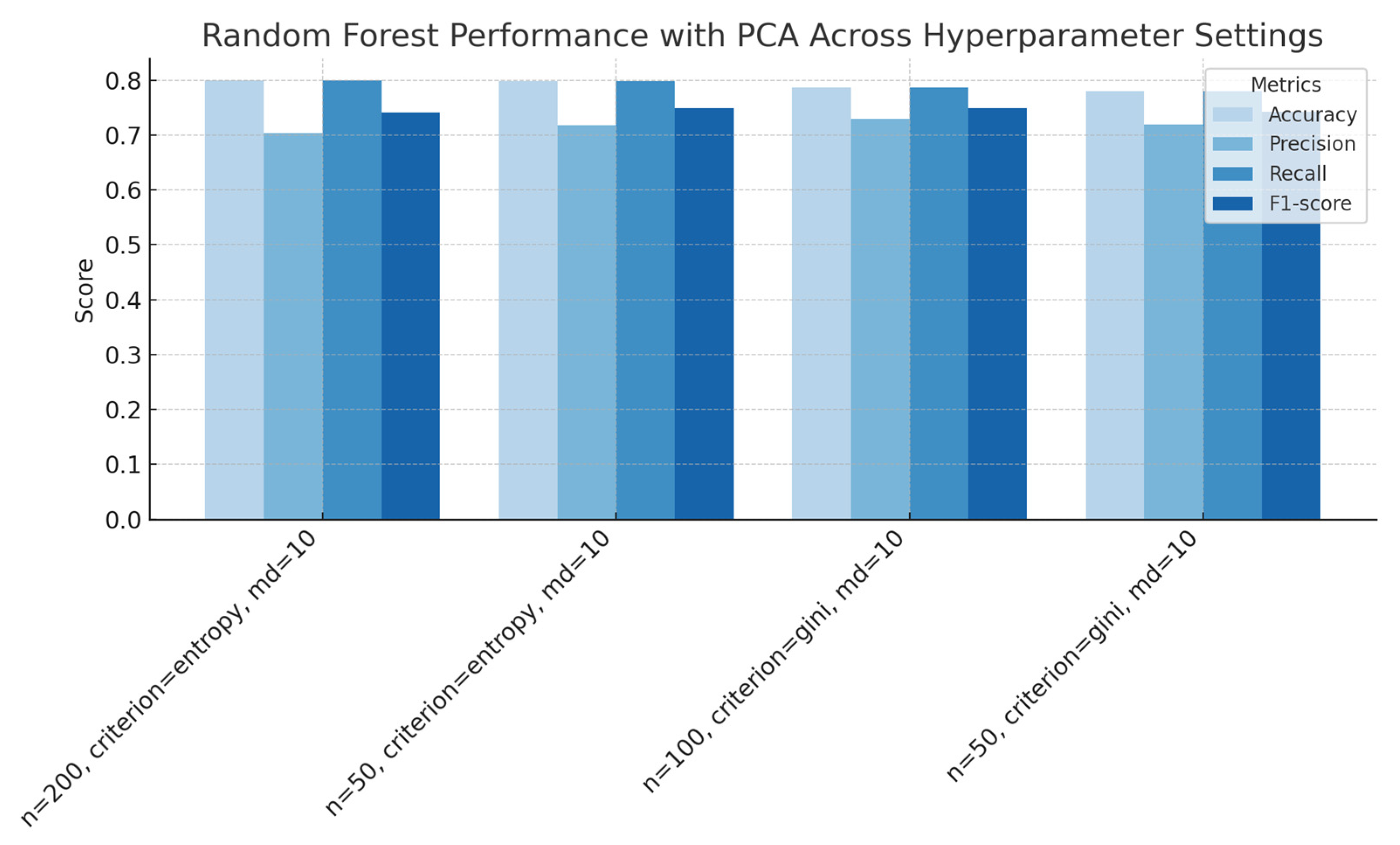
Figure 11 shows Random Forest models on PCA-reduced data under four settings: (a) n = 200, criterion = entropy, max depth = 10, (b) n = 50, criterion = entropy, max depth = 10, (c) n = 100, criterion = gini, max depth = 10 and (d) n = 50, criterion = gini, max depth = 10

The highest accuracy and recall (0.800) occurred with 200 trees and entropy splitting, while maximum precision (0.718) and F1-score (0.748) were achieved with 50 trees and entropy. Using Gini as the split criterion, yielded slightly lower performance, suggesting that entropy-based splitting and larger ensembles better generalized on PCA-reduced features. The optimum model was configured with n estimators = 200, criterion = entropy, and max depth = 10 (

Table 11. Performance metrics for Random Forest with PCA.

Metric	Mean	Standard Deviation	95% Lower Confidence Interval	95% Upper Confidence Interval
Accuracy	0.800	0.071	0.760	0.800
Precision	0.703	0.096	0.6931	0.746
Recall	0.800	0.071	0.7604	0.800
F1-score	0.743	0.072	0.723	0.763

).

4.2.3. K-Nearest Neighbours

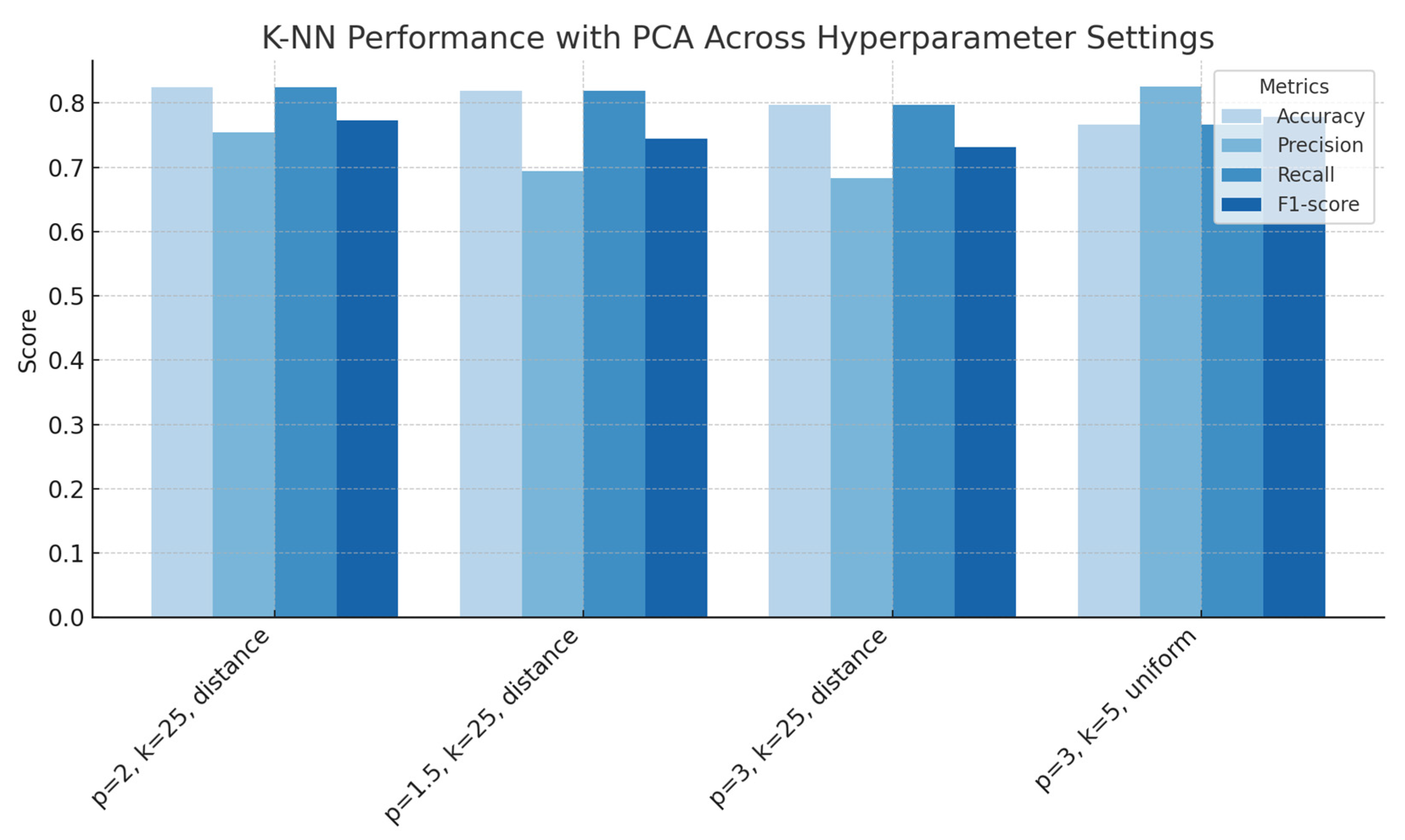
Figure 12 compares the performance of k-Nearest Neighbours (KNN) classifiers after applying Principal Component Analysis (PCA), using four different sets of hyperparameters: (1) p = 2 and k = 25 with distance-based weighting, (2) p = 1.5 and k = 25 with distance-based weighting, (3) p = 3 and k = 25 with distance-based weighting, and (4) p = 3 and k = 5 with uniform weighting. Each group of bars in the figure shows results for one of these configurations, including four evaluation metrics: accuracy, precision, recall, and F1-score.

The best accuracy and recall, both reaching 0.825, are achieved with p = 2, k = 25, and distance weighting. However, this setup gives a moderate precision of 0.754, resulting in an F1-score of 0.773. When the norm is reduced to p = 1.5, accuracy slightly drops to 0.8188 and precision to 0.695. Increasing p to 3, while keeping distance weighting, further lowers accuracy to 0.7975 and the F1-score to 0.732. Finally, using a smaller neighbourhood size of k = 5 with uniform weighting and p = 3 results in the lowest accuracy at 0.766 but the highest precision at 0.825. This indicates that smaller neighbourhoods in the PCA-transformed space tend to favour precision over recall.

A detailed summary of the model’s best performance, including average accuracy, precision, recall, F1-score, standard deviation (SD), and 95% confidence intervals (CI), is provided in the accompanying

Table 12. Performance metrics for k-Nearest Neighbours with PCA.

Metric	Mean	Standard Deviation	95% Lower Confidence Interval	95% Upper Confidence Interval
Accuracy	0.825	0.047	0.812	0.838
Precision	0.754	0.111	0.724	0.785
Recall	0.825	0.047	0.812	0.838
F1-score	0.773	0.062	0.756	0.790

.

4.2.4. Neural Networks

Figure 13 shows the performance of neural network models using ReLU activation and the Adam solver on PCA-transformed data under four different hyperparameter configurations. These include a hidden layer size of 20 with a learning rate of 0.1, a hidden layer size of 10 with a learning rate of 0.1, a hidden layer size of 5 with a learning rate of 0.01, and a hidden layer size of 10 with a learning rate of 0.01. Each group of bars in the figure represents one configuration and displays four evaluation metrics: accuracy, precision, recall, and F1-score.

The best results in terms of recall and accuracy, both reaching 0.784, are achieved when using the largest hidden layer (20 units) with a high learning rate of 0.1. This configuration also gives the highest precision, 0.814, resulting in an F1-score of 0.791. Reducing the hidden layer to 10 neurons while keeping the learning rate at 0.1 causes a slight drop in accuracy and recall, though precision remains high. Lowering the learning rate to 0.01 leads to a gradual decline in all metrics, showing that both the network’s capacity and the learning rate significantly affect performance when combined with PCA-based dimensionality reduction.

A detailed summary of the optimal model’s performance, including average accuracy, precision, recall, F1-score, standard deviation (SD), and 95% confidence intervals (CI), is provided in

Table 13. Performance metrics for Neural Networks with PCA.

Metric	Mean	Standard Deviation	95% Lower Confidence Interval	95% Upper Confidence Interval
Accuracy	0.784	0.047	0.732	0.808
Precision	0.754	0.111	0.724	0.785
Recall	0.784	0.047	0.732	0.808
F1-score	0.773	0.062	0.756	0.790

.

4.2.5. Support Vector Machines

Figure 14 compares the performance of Support Vector Machine (SVM) classifiers applied after PCA dimensionality reduction, under four different hyperparameter settings. These include a linear kernel with C = 0.1, a linear kernel with C = 1.0, an RBF kernel with C = 1.0, and a linear kernel with C = 10.0. Each group of bars in the figure represents one of these configurations and shows four evaluation metrics: accuracy, precision, recall, and F1-score.

The highest accuracy and recall, both reaching 0.813, are observed when using the linear kernel with C = 0.1. However, this setting results in a relatively low precision of 0.6602, producing an F1-score of 0.729. Increasing the value of C to 1.0 under the linear kernel improves performance across most metrics, with recall rising to 0.808, precision to 0.719, and the F1-score to 0.752. When using the RBF kernel with C = 1.0, the model shows balanced performance, achieving an accuracy of 0.788, precision of 0.779, and F1-score of 0.7597. On the other hand, setting a higher regularization parameter of C = 10.0 under the linear kernel shifts the model’s performance toward higher precision (0.805), but with a slight drop in accuracy (0.781).

These results highlight that, after applying PCA, both the choice of kernel and the regularization parameter C play a critical role in shaping the trade-off between precision and recall in SVM models. The detailed performance metrics for the optimal configuration, including mean accuracy, precision, recall, and F1-score, as well as standard deviation (SD) and 95% confidence intervals (CI), are presented in the accompanying

Table 14. Performance metrics for SVM with PCA.

Metric	Mean	Standard Deviation	95% Lower Confidence Interval	95% Upper Confidence Interval
Accuracy	0.813	0.001	0.812	0.814
Precision	0.660	0.001	0.659	0.661.
Recall	0.813	0.001	0.812	0.814
F1-score	0.728	0.001	0.727	0.729

.

4.2.6. LightGBM

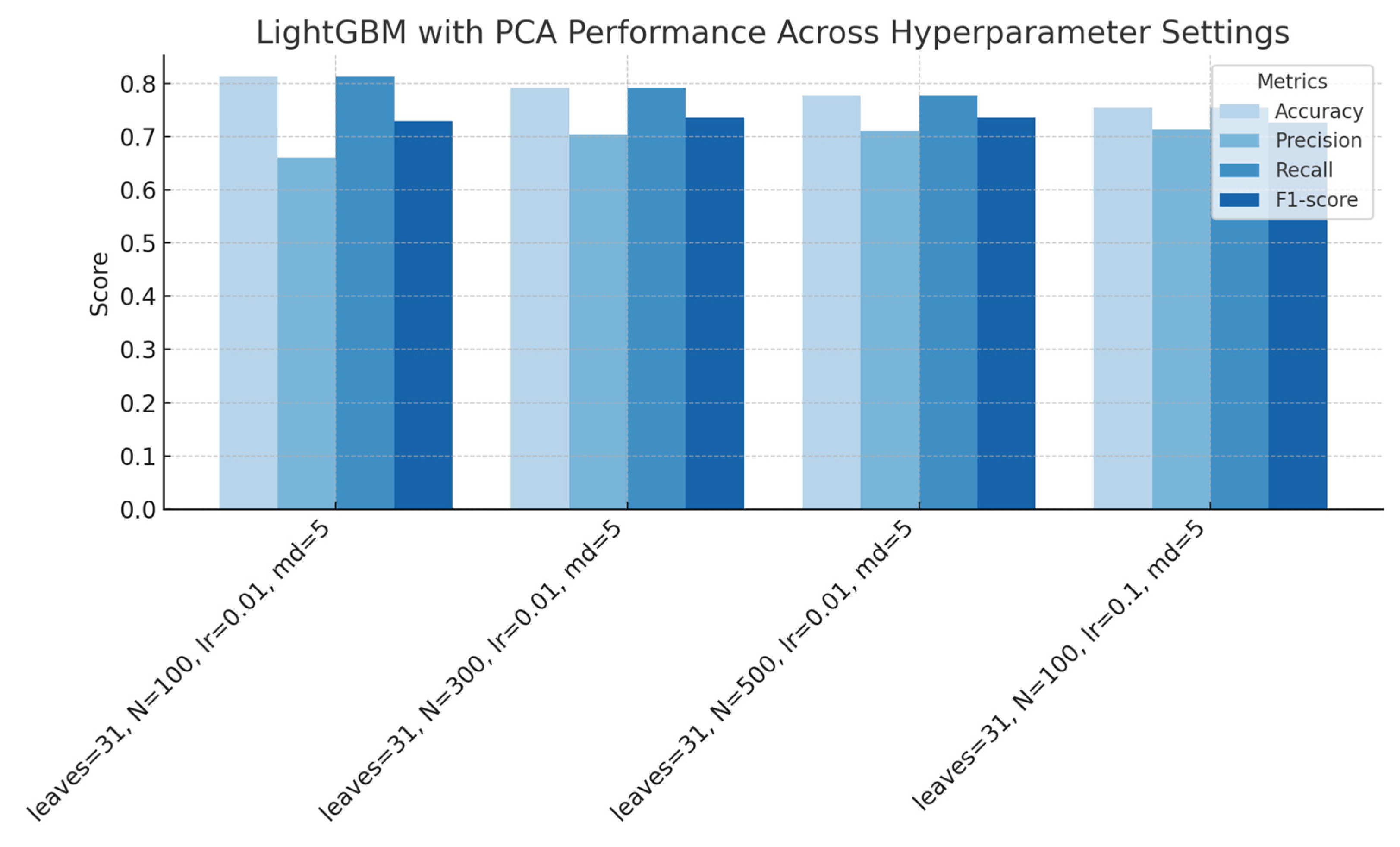
Figure 15 illustrates the performance of LightGBM models after applying Principal Component Analysis (PCA), across four different hyperparameter configurations. These configurations include models with 31 leaves and a maximum depth of 5, while varying the number of estimators and learning rates. Specifically, the setups involve 100, 300, and 500 estimators with a learning rate of 0.01, as well as a configuration with 100 estimators and a higher learning rate of 0.1.

The model configuration with 100 estimators and a learning rate of 0.01 yields the highest accuracy and recall, both reaching 0.813. As the number of estimators increases to 300 and 500, accuracy declines gradually to 0.791 and 0.778, respectively. However, the configuration with 300 estimators delivers the best balance in terms of precision (0.703) and F1-score (0.736). On the other hand, increasing the learning rate to 0.1 while maintaining 100 estimators significantly reduces model performance, with accuracy dropping to 0.754 and the F1-score to 0.726.

These findings suggest that both the size of the ensemble and the learning rate play an important role in determining model effectiveness, particularly when used in conjunction with PCA-based dimensionality reduction. A detailed summary of the optimal configuration’s performance—including average accuracy, precision, recall, F1-score, standard deviation (SD), and 95% confidence intervals (CI)—is provided in the accompanying

Table 15. Performance metrics for LightGBM with PCA.

Metric	Mean	Standard Deviation	95% Lower Confidence Interval	95% Upper Confidence Interval
Accuracy	0.813	0.001	0.812	0.814
Precision	0.660	0.001	0.659	0.661.
Recall	0.813	0.001	0.812	0.814
F1-score	0.728	0.001	0.727	0.729

.

4.2.7. XGBoost

Figure 16 presents the performance of XGBoost models applied to data that has undergone Principal Component Analysis (PCA), evaluated under four distinct hyperparameter settings. These configurations vary in terms of regularization strength (λ), number of estimators (N), learning rate, and maximum tree depth (md). Specifically, the tested combinations include the following: λ = 1 with 500 estimators and a learning rate of 0.05; λ = 5 with 500 estimators and the same learning rate; λ = 5 with 300 estimators and a higher learning rate of 0.1; and λ = 1 with 300 estimators and a learning rate of 0.1. The maximum depth was held constant at 5 in all scenarios.

Among these, the configuration with λ = 1, 500 estimators, and a learning rate of 0.05 produced the strongest overall performance, with accuracy and recall both at 0.761, precision at 0.725, and an F1-score of 0.737. Adjustments such as increasing the regularization strength or decreasing the number of estimators—particularly in combination with a higher learning rate—resulted in modest declines in performance. These findings highlight the continued importance of tuning regularization and ensemble size, even after dimensionality reduction through PCA.

The full results for the best-performing configuration, including the mean values for accuracy, precision, recall, and F1-score—along with their standard deviation (SD) and 95% confidence intervals (CI)—are presented in the corresponding results

Table 16. Performance metrics for XGBoost with PCA.

Metric	Mean	Standard Deviation	95% Lower Confidence Interval	95% Upper Confidence Interval
Accuracy	0.795	0.096	0.763	0.817
Precision	0.782	0.112	0.747	0.809.
Recall	0.790	0.096	0.763	0.817
F1-score	0.781	0.095	0.749	0.802

.

4.2.8. Comparison Between Models with PCA

The table below summarizes the performance of all evaluated models following the application of Principal Component Analysis (PCA). Among all models tested, the k-Nearest Neighbours (k-NN) classifier achieved the highest accuracy and recall, both at 0.825, as well as a strong F1-score of 0.773. This indicates its high capability to correctly classify instances after dimensionality reduction. While the neural network achieved the highest precision at 0.814 and the highest F1-score at 0.791, the overall best performance across all metrics was demonstrated by the k-NN model combined with PCA.

The accompanying

Table 17. Comparison of performance metrics for seven machine learning tools with PCA.

Metric	Accuracy	Precision	Recall	F1-Score
Decision Tree	0.7761	0.790	0.749	0.755
Random Forest	0.813	0.779	0.785	0.776
k-Nearest Neighbours	0.825	0.754	0.825	0.773
Neural Networks	0.784	0.814	0.784	0.791
Support Vector Machines	0.813	0.660	0.813	0.728
LightGBM	0.813	0.660	0.813	0.728
XGBoost	0.761	0.725	0.761	0.737

provides a side-by-side comparison of model performance with and without PCA across four evaluation metrics, using a consistent purple colour scheme for visual clarity. In the accuracy panel, Support Vector Machines (SVM) and k-NN maintain high performance before and after PCA, with k-NN improving from 0.813 to 0.825. LightGBM shows a similar improvement, increasing from 0.798 to 0.813 after applying PCA. In contrast, XGBoost experiences a performance drop, with accuracy decreasing from 0.795 to 0.761. Ensemble tree-based models such as Decision Trees and Random Forests show modest gains in accuracy, while the neural network’s accuracy remains largely unchanged.

In the precision panel, PCA leads to a noticeable decline for XGBoost, LightGBM, and SVM. However, the neural network shows a significant improvement, rising from 0.718 to 0.814. k-NN also benefits, with precision increasing from 0.660 to 0.754. The recall panel follows similar trends to accuracy, with improvements seen in k-NN and SVM after PCA, while XGBoost shows reduced recall.

Finally, the F1-score panel highlights that the models which benefit most from PCA are those that rely on local distance metrics or gradient-based optimization techniques—specifically k-NN, whose F1-score increases from 0.728 to 0.773, the neural network, which improves from 0.731 to 0.791, and the Random Forest model, which rises from 0.743 to 0.776.

4.3. Model Comparison Summary with PCA and Without PCA

Figure 17 presents a side-by-side comparison of model performance before and after applying Principal Component Analysis (PCA), evaluated across four key metrics and visualized using a purple colour scheme for clarity. In the accuracy panel, Support Vector Machines (SVM) and k-Nearest Neighbours (k-NN) maintain strong performance in both scenarios, with k-NN improving slightly from 0.813 to 0.825. LightGBM also shows a notable gain, increasing from 0.798 to 0.813 following PCA. In contrast, XGBoost experiences a drop in accuracy from 0.795 to 0.761. Decision Tree and Random Forest models exhibit modest accuracy improvements, while the neural network’s accuracy remains relatively stable.

In terms of precision, PCA leads to a noticeable reduction for XGBoost, LightGBM, and SVM. However, the neural network sees a substantial increase, with precision rising from 0.718 to 0.814. The k-NN model also benefits, with its precision improving from 0.660 to 0.754. Recall trends largely mirror those observed in accuracy. Both k-NN and SVM show improvement post-PCA, whereas XGBoost demonstrates a decline.

The F1-score results reveal that models which benefit the most from PCA are typically those that depend on local distance-based classification or gradient-driven updates. Notably, the F1-score for k-NN increases from 0.728 to 0.773, the neural network improves from 0.731 to 0.791, and the Random Forest model rises from 0.743 to 0.776.

4.4. SHAP Analysis of Model Predictions

To interpret the contributions of individual wavenumbers to the classification of “Plastic” spectra, we computed SHAP values for our best-performing LightGBM and SVM models. Below we summarize the key findings.

The four heatmaps (Figure 18 and Figure 19) illustrate the mean absolute SHAP values across Raman spectral wavenumbers for both biological and plastic classifications, using two different machine learning methods: SVM (without PCA) and LightGBM (with PCA). For the SVM classifier (without PCA) (Figure 18), the heatmap highlights a pronounced “hot spot” around 1080 cm⁻¹ for both classes, indicating that this wavenumber significantly influences the classification decision.

In contrast, the LightGBM classifier (without PCA) (Figure 19) demonstrates a clear and strong “hot spot” around 700 cm⁻¹ for the plastic class, which suggests that this classifier primarily utilizes this spectral region for differentiating plastics. Additionally, minor but noticeable contributions are evident at several other spectral regions (approximately between 800 and 1200 cm⁻¹), indicating the classifier’s capability to exploit multiple spectral patterns. Similarly, the biological class in the LightGBM heatmap presents scattered yet minor importance across several regions.

Figure 20 indicates that for both the biological (Class 0) and plastic (Class 1) classes, the bar plots of mean SHAP values identify similar key regions around 1080 cm⁻¹ as highly influential. Specifically, wavenumbers around 1078–1082 cm⁻¹ exhibit the highest SHAP importance, clearly marking this spectral region as critical for classification with the SVM model. The similarity between classes indicates that the SVM classifier strongly depends on a narrow, common spectral fingerprint region, relying primarily on subtle intensity differences to differentiate between plastic and biological samples.

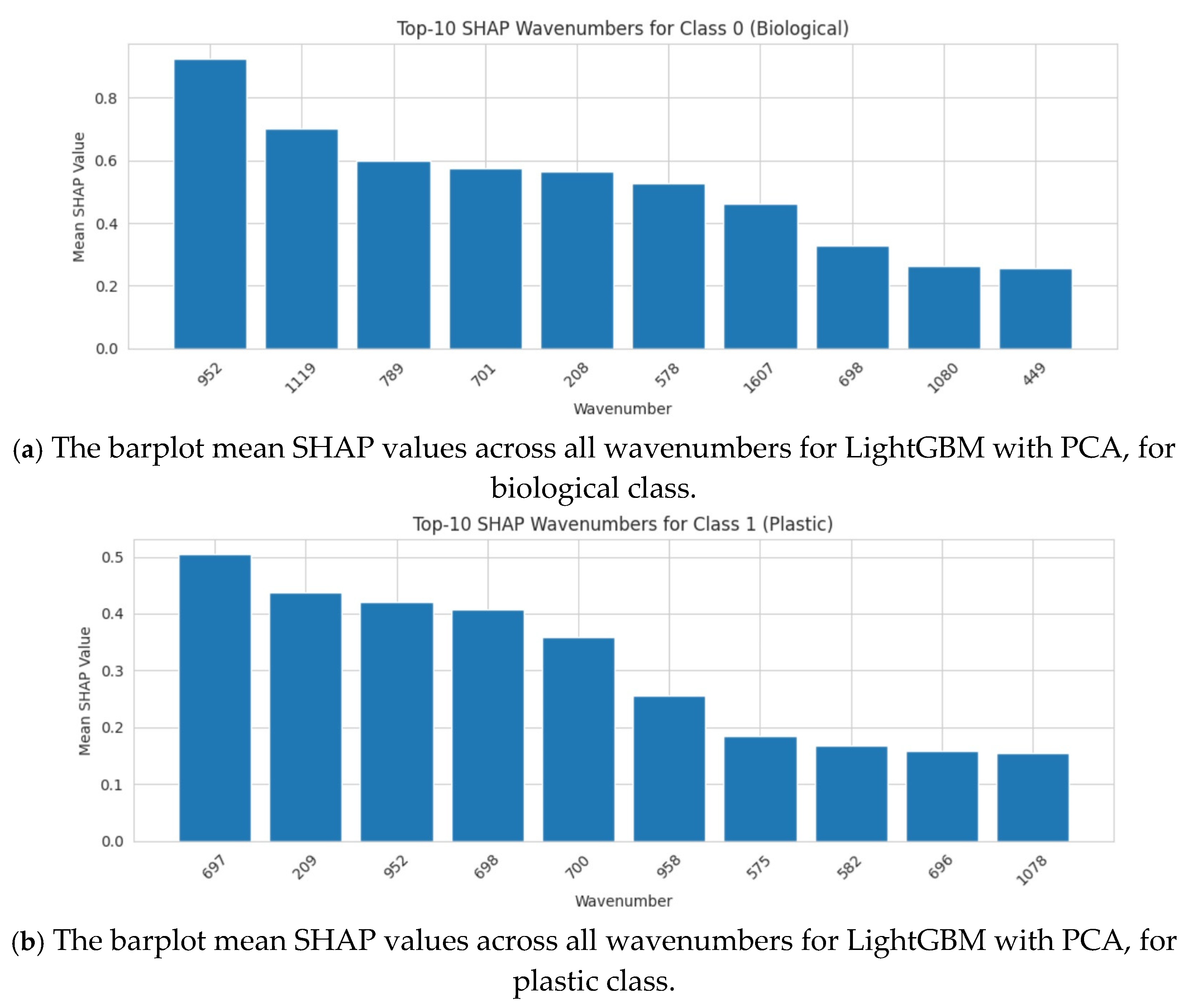
Figure 21 indicates that the LightGBM classifier presents a different and more distributed pattern of feature importance. For the biological class, the highest mean SHAP value is found at 952 cm⁻¹, followed by significant peaks at 1119 cm⁻¹, 789 cm⁻¹, and 701 cm⁻¹, among others. This indicates that the classifier captures a wider range of distinctive biological spectral characteristics, providing a more nuanced classification. For the plastic class, a very clear and dominant peak emerges at 697 cm⁻¹, alongside notable contributions from wavenumbers 209 cm⁻¹, 952 cm⁻¹, and 698 cm⁻¹.

5. Discussion

In recent years, machine learning (ML) has gained popularity in the detection of microplastics and nanoplastics (MNPs). However, most studies have either focused on limited sets of pristine polymer types or prioritized model accuracy without considering transparency. For instance, while studies using cathodoluminescence spectra [18] or sparse [19] autoencoders with Raman data have reported accuracies up to 99%, these results were achieved under highly controlled lab conditions, often excluding weathered plastics and biological materials. Similarly, high-throughput FTIR-based approaches have [22,24] advanced automation but offer little interpretability, functioning largely as black boxes.

Our work advances the field in three key ways. First, we evaluated seven supervised ML algorithms using an open-access Raman spectral library [14] that includes pristine, weathered, and biological materials. This dataset is more representative of real-world samples. By comparing classification performance with and without Principal Component Analysis (PCA), we show that combining robust ML models with spectral preprocessing and explainability techniques creates a powerful microplastic identification tool. Our extensive evaluation across seven model types, optimized via hyperparameters and applied to both raw and PCA-transformed spectra, indicates that ensemble models (LightGBM, Random Forest, XGBoost) and instance-based learners (k-NN) lead in predictive accuracy. SHAP analysis confirms the chemical relevance of spectral regions around 700 cm⁻¹ and 1080 cm⁻¹. Notably, XAI transforms these models into interpretable classifiers, helping domain experts validate and refine spectral assignments.

The SVM model without PCA relies mainly on the 1080 cm⁻¹ region for both classes, whereas LightGBM (also trained without PCA in SHAP analysis) draws from multiple regions, including 700 cm⁻¹ for plastics and 950–1119 cm⁻¹ for biologicals. Although both the plastic and biological classes show high SHAP values around 1080 cm⁻¹ in the SVM model (without PCA), the classifier relies on subtle yet consistent intensity variations within this region to distinguish between them. Specifically, plastic polymers such as PET and PEG typically exhibit stronger, sharper peaks at this band, associated with C–O–C symmetric stretching or phosphate vibrations, whereas biological materials tend to produce broader, lower-intensity signals due to overlapping cellular components like nucleic acids and phospholipids. The SVM capitalizes on these fine-grained spectral differences, effectively separating classes despite the use of a common spectral marker. This highlights the classifier’s sensitivity to intensity morphology, not just peak position. These patterns highlight how different classifiers focus on distinct spectral features. While PCA enables broader feature capture, it may dilute interpretability. By contrast, models trained without PCA—such as SVM—offer more concentrated and explainable feature attributions, preserving the spectral structure.

Correct polymer identification is critical for tracing pollution sources, understanding plastic breakdown, and assessing associated risks. For example, lightweight polyolefins like polyethylene (PE) and polypropylene (PP) float and accumulate at the surface, whereas denser materials like PET and PVC sink and bind pollutants. Misidentification can lead to flawed environmental assessments. By improving model transparency and accuracy, our pipeline strengthens environmental decision-making and supports polluter-pay frameworks [31,32,33].

From a One Health perspective, knowing the polymer type is vital, as toxicity varies with chemical structure and additives. Organisms such as mussels, oysters, and fish can ingest PE, polystyrene, and other polymers along with associated toxins. These substances may bioaccumulate across trophic levels. Polystyrene, for example, crosses the human intestinal barrier more easily than polyamides. Our classifier could be used in seafood testing protocols to detect risk and inform dietary guidelines. Aquaculture operations could also apply this model to monitor water and sediment quality, linking environmental data to food safety. Moreover, our XAI model can identify polymer hotspots in marine ecosystems, enabling more effective public health responses.

The discriminative regions identified by the LightGBM model—also trained on non-PCA-transformed spectra—further support the chemical validity of the predictions. For instance, the 697–701 cm⁻¹ (

Table 18. Raman peaks of polyethylene (PE) and polyvinyl chloride (PVC). Adapted from Jung et al., 2024 [34].

Polymer	Dominant Raman Peaks (cm−1)
Polyethylene (PE)	1062, 1129, 1295, 1416, 1440, 1460, 2727, 2856, 2892
Polyvinyl chloride (PVC)	363, 637, 694, 1119, 1334, 1430, 2935

) region is indicative of C–Cl bending (PVC) or aromatic ring deformations (polystyrene), both characteristic of synthetic plastics. Similarly, the 1080 cm⁻¹ band reflects C–O–C stretching seen in polyesters (e.g., PET) or phosphate groups [30,32]. On the biological side, peaks at 952 cm⁻¹ and 1119 cm⁻¹ are commonly linked to skeletal vibrations in polysaccharides and C–C/C–N stretching in cellulose or proteins, respectively. Additional contributions from 789 cm⁻¹ (nucleic acid ring breathing), 209 cm⁻¹ (low-frequency skeletal modes), and 698 cm⁻¹ further illustrate how the model integrates both low- and mid-range Raman features to differentiate classes. These spectral assignments align with known Raman shifts in the literature [30], reinforcing the chemical interpretability of the XAI outputs. Combined with the SHAP, Table 18 gives researchers a concise, data-driven roadmap of feature importance that clarifies which factors most strongly influence the model’s predictions.

This methodology can embedded in a system, which can serve several day-to-day needs: customs officers at ports can test container wash-water on the spot and print reports that satisfy EU plastic-litter rules; beach-clean volunteers working with NGOs can scan debris as they collect it, with the device highlighting hazardous plastics such as PVC or PU so these items are removed first; and operators in municipal wastewater plants can attach a flow-through cell, receive a fresh microplastic reading every minute, and adjust treatment steps immediately. Together, these examples show how our method becomes a practical, field-ready decision tool.

Building on this foundation, future research will expand the spectral database to include nanoplastics, polymer blends, and coated samples, improving generalizability. We also plan to incorporate FTIR and hyperspectral imaging into a unified XAI framework, enabling broader chemical detection and reducing error rates. For real-time, on-site monitoring, we will deploy our pipeline on portable Raman spectrometers with edge computing, allowing non-experts to conduct automated surveys and receive immediate, interpretable results. Finally, federated and active learning will be explored to continuously improve the system while maintaining privacy, and to connect polymer classification outputs with ecotoxicological models through explainable QSAR approaches.

References

1. Thompson, R.C.; Courtene-Jones, W.; Boucher, J.; Pahl, S.; Raubenheimer, K.; Koelmans, A.A. Twenty years of microplastic pollution research—What have we learned? Science 2024, 386, eadl2746. [Google Scholar] [CrossRef] [PubMed]
2. Biswas, R.; Debnath, C.; Barua, R.; Samanta, I. Microplastics: A One Health priority agenda. One Health Bull. 2024, 4, 104–109. [Google Scholar] [CrossRef]
3. Thompson, R.C.; Olsen, Y.; Mitchell, R.P.; Davis, A.; Rowland, S.J.; John, A.W.G.; McGonigle, D.; Russell, A.E. Lost at Sea: Where Is All the Plastic? Science 2004, 304, 838. [Google Scholar] [CrossRef]
4. Rashid, S.; Majeed, L.R.; Mehta, N.; Radu, T.; Martín-Fabiani, I.; Bhat, M.A. Microplastics in terrestrial ecosystems: Sources, transport, fate, mitigation, and remediation strategies. Euro Mediterr. J. Environ. Integr. 2025, 10, 2633–2659. [Google Scholar] [CrossRef]
5. Van Melkebeke, M. Exploration and Optimization of Separation Techniques for the Removal of Microplastics From Marine Sediments During Dredging Operations. Master’s Thesis, Ghent University, Gent, Belgium, 2019. [Google Scholar]
6. Morrison, M.; Trevisan, R.; Ranasinghe, P.; Merrill, G.B.; Santos, J.; Hong, A.; Edward, W.C.; Jayasundara, N.; Somarelli, J.A. A growing crisis for One Health: Impacts of plastic pollution across layers of biological function. Front. Mar. Sci. 2022, 9, 705. [Google Scholar] [CrossRef]
7. Stapleton, M.J. FIH Microplastics as an emerging contaminant of concern: Sources and implications. Bioengineered 2023, 14, 2244754. [Google Scholar] [CrossRef] [PubMed]
8. Procopio, A.C.; Soggiu, A.; Urbani, A.; Roncada, P. Interactions between microplastics and microbiota in a One Health perspective. One Health 2025, 20, 101002. [Google Scholar] [CrossRef]
9. Eriksen, M.; Lebreton, L.C.; Carson, H.S.; Thiel, M.; Moore, C.J.; Borerro, J.C.; Galgani, F.; Ryan, P.G.; Reisser, J. Plastic Pollution in the World’s Oceans: More than 5 Trillion Plastic Pieces Weighing over 250,000 Tons Afloat at Sea. PLoS ONE 2014, 9, e111913. [Google Scholar] [CrossRef]
10. Jambeck, J.R.; Geyer, R.; Wilcox, C.; Siegler, T.R.; Perryman, M.; Andrady, A.; Narayan, R.; Law, K.L. Plastic waste inputs from land into the ocean. Science 2015, 347, 768–771. [Google Scholar] [CrossRef]
11. Prata, J.C.; da Costa, J.P.; Lopes, I.; Andrady, A.L.; Duarte, A.C.; Rocha-Santos, T. A One Health perspective of the impacts of microplastics on animal, human and environmental health. Sci. Total Environ. 2021, 777, 146094. [Google Scholar] [CrossRef]
12. Ma, H.; Pu, S.; Liu, S.; Bai, Y.; Mandal, S.; Xing, B. Microplastics in aquatic environments: Toxicity to trigger ecological consequences. Environ. Pollut. 2020, 261, 114089. [Google Scholar] [CrossRef]
13. Zhang, Y.; Zhang, D.; Zhang, Z. A Critical Review on Artificial Intelligence—Based Microplastics Imaging Technology: Recent Advances, Hot-Spots and Challenges. Int. J. Environ. Res. Public Health 2023, 20, 1150. [Google Scholar] [CrossRef]
14. Miller, E.A.; Yamahara, K.M.; French, C.; Spingarn, N.; Birch, J.M.; Van Houtan, K.S. A Raman spectral reference library of potential anthropogenic and biological ocean polymers. Sci. Data 2022, 9, 780. [Google Scholar] [CrossRef] [PubMed]
15. Jin, H.; Kong, F.; Li, X.; Shen, J. Artificial intelligence in microplastic detection and pollution control. Environ. Res. 2024, 262, 119812. [Google Scholar] [CrossRef] [PubMed]
16. Yang, J.; Peng, Z.; Sun, J. A review on advancements in atmospheric microplastics research: The pivotal role of machine learning. Sci. Total Environ. 2024, 945, 173966. [Google Scholar] [CrossRef] [PubMed]
17. Hu, B.; Dai, Y.; Zhou, H.; Sun, Y.; Yu, H.; Dai, Y.; Wang, M.; Ergu, D.; Zhou, P. Using artificial intelligence to rapidly identify microplastics pollution and predict microplastics environmental behaviors. J. Hazard. Mater. 2024, 474, 134865. [Google Scholar] [CrossRef]
18. Höppener, E.M.; Shahmohammadi, M.S.; Parker, L.A.; Henke, S.; Urbanus, J.H. Classification of (micro)plastics using cathodoluminescence and machine learning. Talanta 2023, 253, 123985. [Google Scholar] [CrossRef]
19. Luo, Y.; Su, W.; Xu, X.; Xu, D.; Wang, Z.; Wu, H.; Chen, B.; Wu, J. Raman Spectroscopy and Machine Learning for Microplastics Identification and Classification in Water Environments. IEEE J. Sel. Top. Quantum Electron. 2023, 29. [Google Scholar] [CrossRef]
20. Chaczko, Z.; Wajs-Chaczko, P.; Tien, D.; Haidar, Y. Detection of Microplastics Using Machine Learning. In Proceedings of the ICMLC 2019, Kobe, Japan, 7–10 July 2019; pp. 1–8. [Google Scholar] [CrossRef]
21. Weber, F.; Zinnen, A.; Kerpen, J. Development of a machine learning-based method for the analysis of microplastics in environmental samples using Raman spectroscopy. Microplast. Nanoplast. 2023, 3, 9. [Google Scholar] [CrossRef]
22. Kedzierski, M.; Falcou-Préfol, M.; Kerros, M.E.; Henry, M.; Pedrotti, M.L.; Bruzaud, S. A machine learning algorithm for high throughput identification of FTIR spectra: Application on microplastics collected in the Mediterranean Sea. Chemosphere 2019, 234, 242–251. [Google Scholar] [CrossRef]
23. Liu, C.; Zong, C.; Chen, S.; Chu, J.; Yang, Y.; Pan, Y.; Yuan, B.; Zhang, H. Machine learning-driven QSAR models for predicting the cytotoxicity of five common microplastics. Toxicology 2024, 508, 153918. [Google Scholar] [CrossRef]
24. Yan, X.; Cao, Z.; Murphy, A.; Qiao, Y. An ensemble machine learning method for microplastics identification with FTIR spectrum. J. Environ. Chem. Eng. 2022, 10, 108130. [Google Scholar] [CrossRef]
25. Qiu, Y.; Li, Z.; Zhang, T.; Zhang, P. Predicting aqueous sorption of organic pollutants on microplastics with machine learning. Water Res. 2023, 244, 120503. [Google Scholar] [CrossRef] [PubMed]
26. Miller, E.A.; Yamahara, K.M.; French, C.; Spingarn, N.; Birch, J.; Van Houtan, K.S. A Raman Spectral Reference Library of Potential Anthropogenic and Biological Ocean Polymers. Dataset. Open Science Framework, 28 November 2022. [Google Scholar] [CrossRef]
27. Jolliffe, I.T.; Cadima, J. Principal component analysis: A review and recent developments. Philos. Trans. R. Soc. A 2016, 374, 20150202. [Google Scholar] [CrossRef] [PubMed]
28. Wold, S.; Esbensen, K.; Geladi, P. Principal component analysis. Chemom. Intell. Lab. Syst. 1987, 2, 37–52. [Google Scholar] [CrossRef]
29. Hastie, T.; Tibshirani, R.; Friedman, J. The Elements of Statistical Learning: Data Mining, Inference, and Prediction, 2nd ed.; Springer: New York, NY, USA, 2009. [Google Scholar]
30. Krafft, C.; Schie, I.W.; Meyer, T.; Schmitt, M.; Popp, J. Developments in spontaneous and coherent Raman scattering microscopic imaging for biomedical applications. Chem. Soc. Rev. 2016, 45, 1819–1849. [Google Scholar] [CrossRef]
31. Hermabessiere, L.; Dehaut, A.; Paul-Pont, I.; Lacroix, C.; Jezequel, R.; Soudant, P.; Duflos, G. Occurrence and effects of plastic additives on marine environments and organisms: A review. Chemosphere 2017, 182, 781–793. [Google Scholar] [CrossRef]
32. Cole, M.; Lindeque, P.; Halsband, C.; Galloway, T.S. Microplastics as contaminants in the marine environment: A review. Mar. Pollut. Bull. 2011, 62, 2588–2597. [Google Scholar] [CrossRef]
33. Schwabl, P.; Köppel, S.; Königshofer, P.; Bucsics, T.; Trauner, M.; Reiberger, T.; Liebmann, B. Detection of Various Microplastics in Human Stool. Ann. Intern. Med. 2019, 171, 453–457. [Google Scholar] [CrossRef]
34. Jung, E.S.; Choe, J.H.; Kim, J.S.; Ahn, D.W.; Yoo, J.; Choi, T.M.; Pyo, S.G. Quantitative Raman analysis of microplastics in water using peak area ratios for concentration determination. NPJ Clean. Water 2024, 7, 104. [Google Scholar] [CrossRef]
Figure 1. Adjusted global plastic production (1950–2019) and projection (2020–2060).
Microplastics 04 00051 g001
Figure 2. Diagrammatic presentation of the flow chart of the methodological procedure.
Microplastics 04 00051 g002
Figure 3. Decision Trees performance across splitting criteria and sample parameters, showing accuracy, precision, recall and F1-score for each configuration.
Microplastics 04 00051 g003
Figure 4. Random Forest performance across different numbers of estimators and splitting criteria (Gini versus log-loss), with a fixed maximum depth of 10, showing accuracy, precision, recall and F1-score for each configuration.
Microplastics 04 00051 g004
Figure 5. k-Nearest Neighbours performance across with a variety of hyperparameters (number of neighbours, distance norms, weighing schemes), showing accuracy, precision, recall and F1-score for each configuration.
Microplastics 04 00051 g005
Figure 6. Neural Networks performance across with a variety of hyperparameters (activation = relu, varying hidden layer size, initial learning rate, and solver), showing accuracy, precision, recall, and F1-score for each configuration.
Microplastics 04 00051 g006
Figure 7. Support Vector Machines performance across kernel types and regularization parameters, showing accuracy, precision, recall and F1-score for each configuration.
Microplastics 04 00051 g007
Figure 8. LightGBM performance across hyperparameter settings (regularization, number of estimators, learning rate, and maximum depth), showing accuracy, precision, recall, and F1-score for each configuration.
Microplastics 04 00051 g008
Figure 9. XGBoost performance across hyperparameter settings (regularization, number of estimators, learning rate, and maximum depth), showing accuracy, precision, recall and F1-score for each configuration.
Microplastics 04 00051 g009
Figure 10. Decision Trees performance with application of PCA across hyperparameter settings (splitting criterion, maximum depth, minimum samples split, and minimum samples leaf), showing accuracy, precision, recall, and F1-score for each configuration.
Microplastics 04 00051 g010
Figure 11. Random Forest performance with PCA across hyperparameter settings (number of estimators, splitting criterion, and maximum depth), showing accuracy, precision, recall, and F1-score for each configuration.
Microplastics 04 00051 g011
Figure 12. k-Nearest Neighbours performance with PCA across hyperparameter settings (number of neighbours, distance norms, weighing schemes), showing accuracy, precision, recall and F1-score for each configuration.
Microplastics 04 00051 g012
Figure 13. Neural Networks performance with PCA across with a variety of hyperparameters (activation = relu, varying hidden layer size, initial learning rate, and solver), showing accuracy, precision, recall, and F1-score for each configuration.
Microplastics 04 00051 g013
Figure 14. Support Vector Machines performance with PCA across kernel types and regularization parameters, showing accuracy, precision, recall, and F1-score for each configuration.
Microplastics 04 00051 g014
Figure 15. LightGBM performance with PCA across hyperparameter settings (regularization, number of estimators, learning rate, and maximum depth), showing accuracy, precision, recall, and F1-score for each configuration.
Microplastics 04 00051 g015
Figure 16. XGBoost performance with PCA across hyperparameter settings (regularization, number of estimators, learning rate and maximum depth), showing accuracy, precision, recall and F1-score for each configuration.
Microplastics 04 00051 g016
Figure 17. Model Comparison based on Accuracy and F1-Score without PCA and with PCA.
Microplastics 04 00051 g017
Figure 18. The heatmap of mean absolute SHAP values across all wavenumbers for SVM without PCA, for both classes, plastic and biological.
Microplastics 04 00051 g018
Figure 19. The heatmap of mean absolute SHAP values across all wavenumbers for LightGBM without PCA, for both classes, plastic and biological.
Microplastics 04 00051 g019
Figure 20. The barplot mean SHAP values across all wavenumbers for SVM without PCA, for both classes, plastic and biological.
Microplastics 04 00051 g020
Figure 21. The barplot mean SHAP values across all wavenumbers for LightGBM with PCA, for both classes, plastic and biological.
Microplastics 04 00051 g021