Abstract
The focus in microplastic research has shifted from marine ecosystems towards freshwater ecosystems. Still, most studies are based on small sample numbers, both spatially and temporally. Little is known about the spatiotemporal variability of microplastics (MPs) in large river systems such as the Rhine River, Germany. Within our study, we performed four cross-sectional sampling campaigns at two sites in the Rhine River, at Koblenz and Emmerich, involving depth-distributed sampling over a particle size range from 10 µm to 25 mm. For plastic particle analysis, we used both optical and thermoanalytical approaches to determine mass-based polymer concentrations. Our results show that MP variability within the water column is complex, but mostly follows the particles density: the ratio between superficial MPs concentration and mean concentration of the verticals was >1 for lighter polymers with a density below 1.04 g/cm3 and <1 for polymers with a density above 1.04 g/cm3 among all size classes with only a few exceptions, even though the Rouse theory would indicate a more homogeneous distribution for small particle sizes. Large sampling volumes are essential, particularly for larger MP particles, as the coefficient of variation rises with particle size. At our study sites, no significant lateral variation was apparent, while during a flood event, MP concentrations were significantly higher than during low and mean water stages. This study is the first to (i) gain insights into cross-sectional MPs distribution in the Rhine River and (ii) account for particle mass concentrations, and thus lays the foundation for potential future MPs flux monitoring.
1. Introduction
The pollution of fluvial freshwater systems with microplastics (MPs) is a growing field of concern [1]. MPs are commonly defined as plastic particles with diameters between 1 µm and 5 mm and can be subdivided into primary (intentionally produced polymers within this size range) and secondary MPs (stemming from fragmentation) [2]. MPs occur in a variety of sizes, shapes, colours, and densities from a variety of sources and can thus be characterised as a highly heterogeneous mixture of artificial particles [3]. MPs, as ubiquitous pollutants, pose various risks to the environment, such as uptake by organisms and a transfer to higher trophic levels or an adsorption and enrichment of pollutants at the particle’s surface [4,5,6,7].
Riverine transport of MPs has recently gained attention within the scientific community [8,9,10,11,12,13]. Transport is highly relevant as it causes the repositioning of MPs from sources to sinks on a river course with lateral and vertical movements along its way. To date, little is known about the complex transport pathways and rates of MPs in rivers, which are essential to assess riverine MPs contamination in a larger context. It becomes apparent in recent literature that MPs transport in large rivers seems to be comparably variable in time and space, as is well known for the transport of suspended sediments [9,14,15,16,17,18,19].
The adoption of existing knowledge from geomorphology is slowly gaining attention in the scientific community [9,10,11,13,17]. For the variation of MPs concentration in space, little is known, as sampling with a high spatial resolution is a challenging task, particularly in large rivers. Recent research indicates that MPs transport is not limited to the water surface, but rather a complex phenomenon with different MPs transport rates at different water depths [13,15,20,21,22,23]. Riverine transport of MP particles on the hydraulic scale is determined by the particle density, shape, and size, which affect particle sinking or rising [10]. Breakdown and degradation, (homo/hetero)-aggregation or biofilm formation on the particle’s surface can occur [8,24,25,26] and therefore modify the hydraulic characteristics of MP particles with time. Also, hydraulic and morphologic parameters of the river itself influence particles’ movement [11,26]. Cowger et al. [15] showed that all gradients in concentration depth profiles are theoretically possible, and it therefore might fall short to rely only on surface sampling. Rather, it could be necessary to adapt sampling strategies so that depth-distributed measurements along cross profiles reveal the vertical and horizontal distribution of MPs, as is the standard in suspended sediment transport measurements [15,27]. To date, only a few studies have performed depth-distributed sampling of MPs within rivers [13,14,20,21,26,28,29].
Despite the large number of case studies, many uncertainties remain, and the comparability among studies is questionable [17,30]. For the sampling of MPs in the aqueous phase, large sample volumes are needed because of the low concentrations of MPs in river water [11]. Too small sample volumes can lead to a biased MPs concentration determination. Therefore, different methods are applied, which can be divided into bulk-sampling (collection of a distinct volume of water without reducing the fluid) and volume-reduced sampling (reducing the water volume by, e.g., filtration of the particles of interest [31]). Each sampling technique has its advantages and limitations (e.g., sample volume, cut-off size, or isokinetic measurement), yet no ideal sampling method exists to date that combines all advantages [11,32]. Large uncertainties are assumed for current sampling strategies, mainly relying on surface sampling [33].
Most freshwater MPs studies estimate the number of particles found per sampling volume, whereas MPs concentration by means of mass per volume is seldom reported [32]. This is mainly caused by analytical issues of MPs identification and quantification [31]. Estimates based on mass are more robust, e.g., against further fragmentation during the sample preparation, and significant discrepancies have been noted between MPs number and the MPs mass [17,34,35,36,37].
For the Rhine River, several MPs studies have been published, of which all investigated the aqueous phase using filter nets with a mesh size of 300 µm (see Table 1 for a summary of the main results from these studies). In general, all studies except one [38] detected an increasing trend of MPs concentration along the river course, with the highest concentrations of primary MPs found in the Ruhr area and dropping values close to the estuary region at Zuilichem, 90 km downstream of Emmerich [39,40,41,42]. No seasonal trends were observed, while a positive relationship between discharge and MPs concentration was detected [41]. Cross-sectional aspects were regarded only in one study [39] and only for the water surface; furthermore, not at all sampling sites. Mani et al. [39] and Mani and Burkhardt-Holm [41] investigated cross profiles and seasonal trends, respectively, but only sampled the water surface. So far, no investigation of depth-distributed MPs concentration has been performed in the Rhine River [41].

Table 1.
Studies investigating aqueous MPs contamination in the Rhine River.
In our study, we aim to contribute to the often-demanded need for depth-distributed MPs sampling and event-related sampling to address the knowledge gap of the cross-sectional distribution of MPs in rivers [11,13,15,23]. Based on the previous findings described above, we expect that (a) distinct concentration depth profiles of different polymers can be detected by depth-distributed sampling at two sampling sites (Koblenz and Emmerich) along the Rhine River, (b) the concentration depth profiles will vary with both particle size and particle density, and (c) sampling without including cross-sectional knowledge at a distinct site may lead to not representative MPs concentrations. This study is the first in-depth analysis of MP concentrations in cross-profiles including depth-distributed sampling in the Rhine River, Europe’s busiest waterway. It thus constitutes an essential contribution to the research of spatiotemporal variability of MPs in large river systems, which feeds back to the development of sampling design for MPs monitoring of such river systems.
2. Materials and Methods
2.1. Study Sites
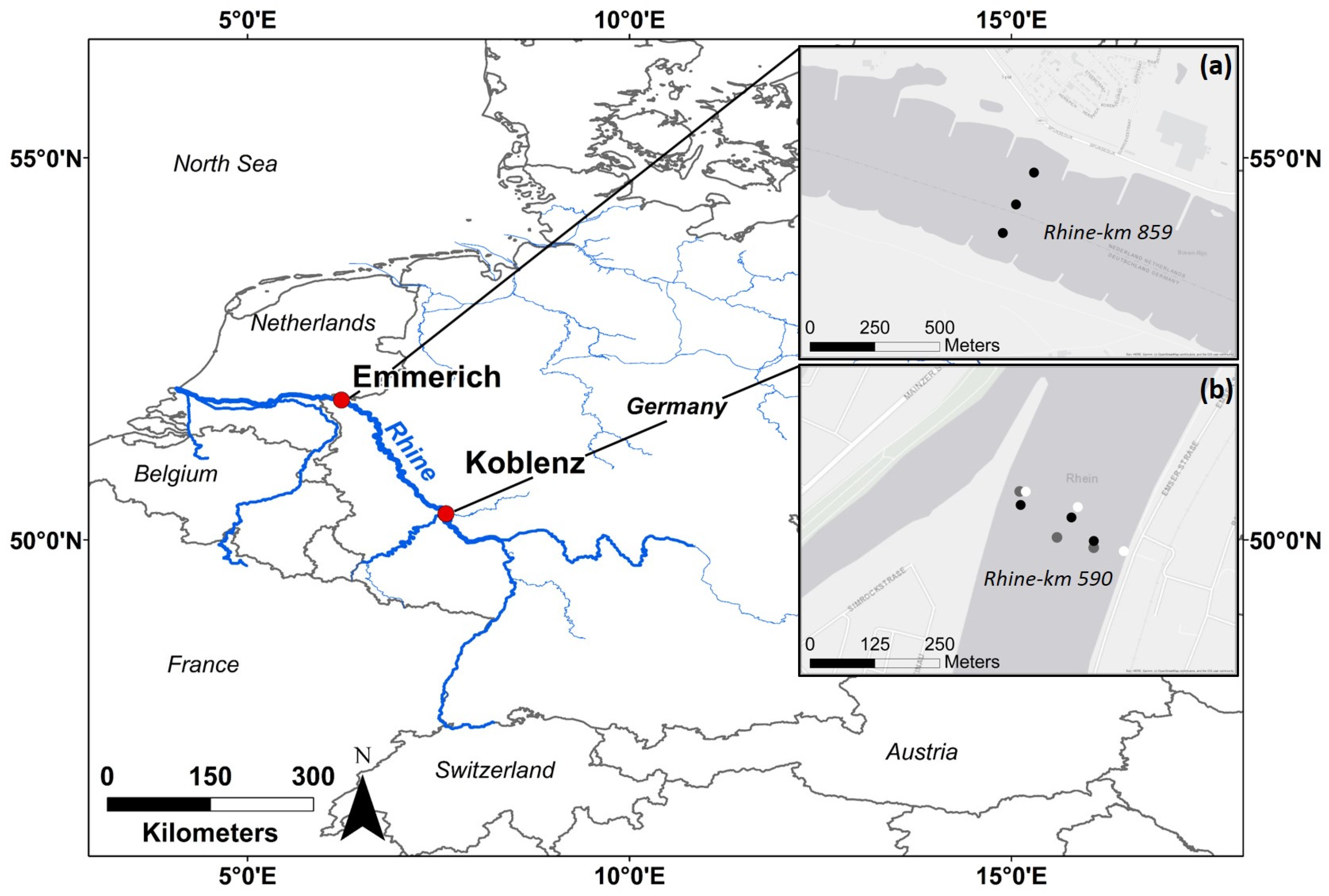
This study was conducted at two sampling sites along the Rhine River in Germany: the main sampling site was located in Koblenz (Rhine km 590), and an additional site was located 269 km downstream in Emmerich (Rhine km 859) close to the Dutch/German border (see Figure 1). Koblenz is located within the Middle-Rhine basin, where a pluvio-nival discharge regime predominates. The mean annual discharge is 1660 m3/s, and the contributing catchment area has about 109,806 km2 [43]. Emmerich is located in the Lower-Rhine basin, with a complex discharge regime, a mean annual discharge of 2260 m3/s, and a contributing catchment area of about 159,555 km2 [43]. The Ruhr area, the most densely populated region in Western Germany, with multiple industrial plants, is situated between the two sampling sites [44]. Sampling sites were chosen mainly due to logistical reasons and accessibility: for the campaigns, both (i) a large vessel with a crane and (ii) nearby monitoring of discharge and suspended sediment concentration (SSC) were needed. At both sites, sampling vessels of the German Waterways and Shipping Authority (WSV) could be used, and nearby monitoring stations from the WSV were used for suspended sediment monitoring [45].
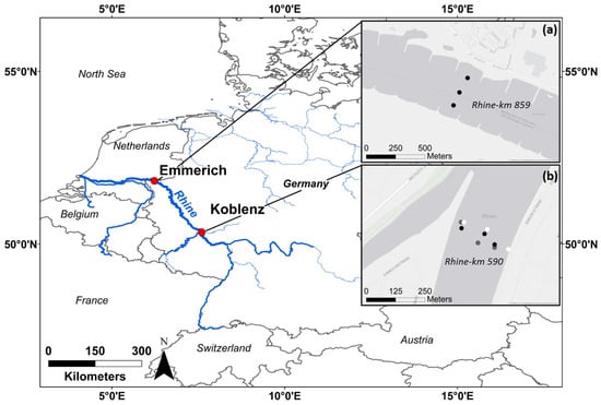
Figure 1.
Study sites and sampling points in the river cross-section. (a) shows the study site at Emmerich, (b) shows the study site at Koblenz. Different colours represent different sampling dates: black points represent sampling during mean flow conditions (8 September 2021), grey points represent sampling during low water conditions (23 November 2021), and white points represent sampling during a flood event (16 March 2023). Sources of the basemaps in (a,b): Esri, HERE, Garmin, FAO, NOAA, USGS, © OpenStreetMap contributors, and the GIS User Community.
2.2. MP Sampling
Two stationary sampling devices have been developed to combine the advantages of two measurement principles: The main device is based on synchronous sampling at three depths via filter nets and has the advantage of gaining large sample volumes in a short time. The supplementary device was a filter cascade, which is based on pump filtration and has the advantage of sampling small-sized particles, which cannot be covered by the filter nets with mesh sizes of 300 µm [46]. Mesh sizes < 300 µm for the filter nets were not applicable due to high backwater (see Section 2.2.1), which is why we additionally used a pump filtration device. Both methods fall into the category of volume-reduced sampling methods.
2.2.1. Depth-Distributed Sampling with 300 µm Filter Nets
For the depth-distributed sampling, a setup based on 6 filter nets was constructed with a mesh size of 300 µm (Hydrobios GmbH, Kiel, Germany), each equipped with a flow-meter for sampling volume measurement (see Figure 2). The nets were fixed to a steel cable at three depths for MPs sampling at the same time. At each depth, a pair of nets allowed for redundant sampling. At the lower end of the cable, a weight of 100 kg prevented the construction from drifting due to the river flow. The lowermost nets were positioned about 50 cm above the river bed, the middle nets were adjusted according to the water depth to sample the middle of the water column at each vertical, and the uppermost nets sampled, supported by two floating bodies, the water surface and below. The construction was lowered at three lateral positions along the river cross-sections with a crane from a vessel. The sampling device was inspired by a similar construction used by Liedermann et al. [20] in the Danube River, but adapted to the conditions at the sampling site.
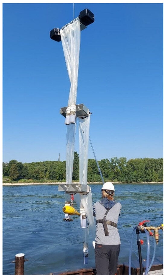
Figure 2.
Depth-distributed sampling device based on 300 µm filter nets (Hydrobios GmbH, Kiel, Germany).
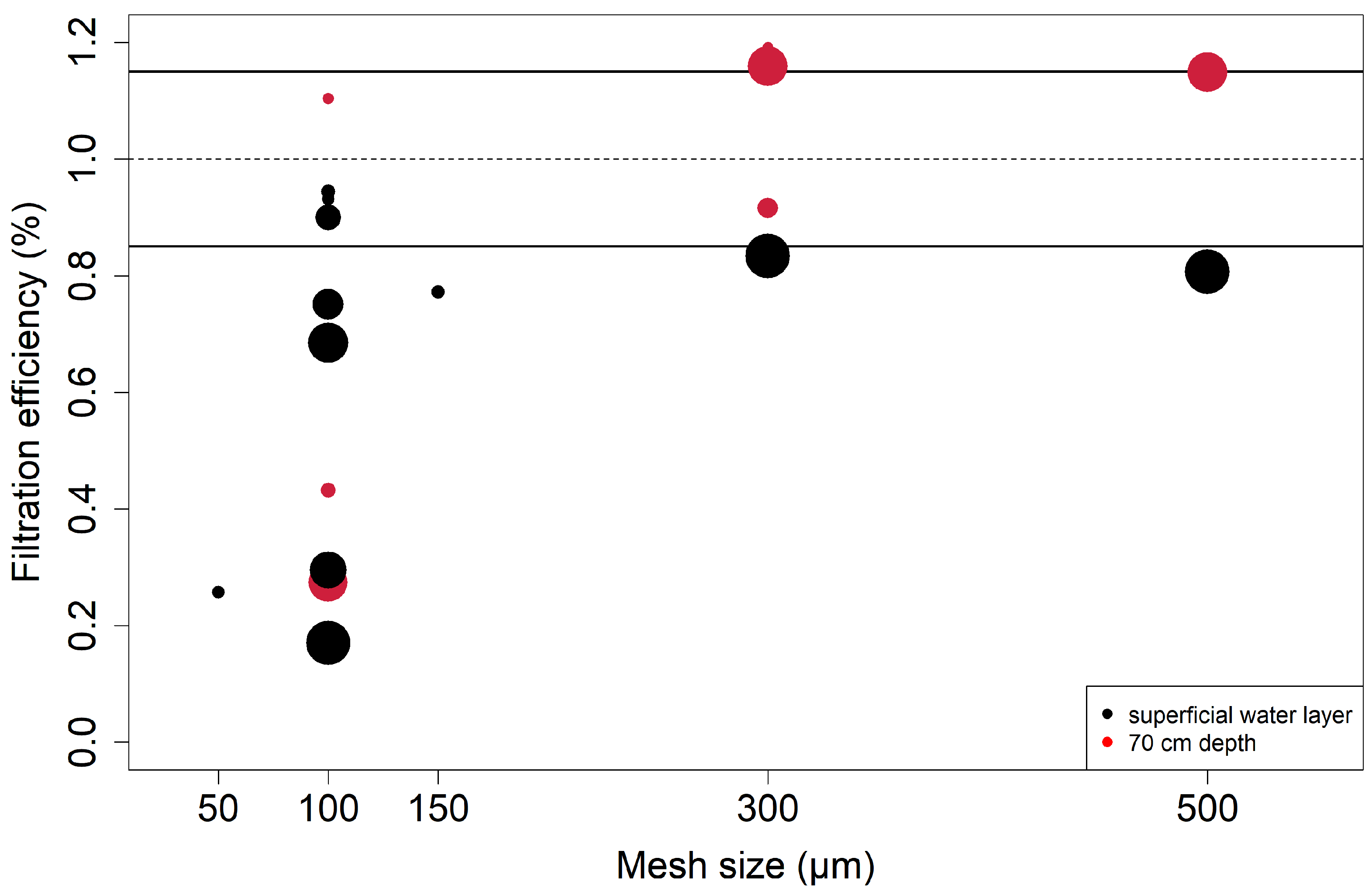
Although all existing studies in the Rhine River used filter nets with a mesh size of ≥300 µm, preliminary tests were performed to determine the optimal mesh size for this study. The best compromise between the smallest cut-off size and tolerable backwater, which might distort the inflow of particles, was determined [20,47,48]. To this end, measurements were performed with a flowmeter inside and outside the net to calculate the filtration efficiency, i.e., the percentage of flow velocity within the filter net relative to the flow velocity outside of the filter net [11,20,31]. Different mesh sizes (50, 100, 150, 300, and 500 µm) were compared at both the water surface and 70 cm below the water surface, and with different SSC (minimum of 4.2 and maximum of 17.1 mg/L), to test for differing discharge scenarios. A filtration efficiency of 85% was deemed acceptable, as a mesh size of 300 µm yielded the best compromise between the smallest cut-off size and the highest filtration efficiency (see Figure 3).
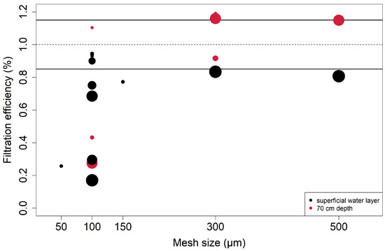
Figure 3.
Results of experiments to assess the filtration efficiency (%) of different mesh sizes (µm) at different SSC values (calibrated FNU). Black points mark surface samples, and red points mark samples at 70 cm water depth. The size of the points represents the relative SSC value during the experiments, which ranged between 4.2 and 17.1 mg/L. The dotted line marks a 100% filtration efficiency, meaning that filtration volume is equal with and without a net (no backwater effect). The black lines mark the range of 15% deviation, which was deemed acceptable within this study.
2.2.2. Near-Surface Sampling with a Filter Cascade
Additional information about MPs with particle sizes < 300 µm was acquired by the construction of a portable filter cascade using pressurised pump filtration (see Figure 4). The cascade consists of three basket filters of 100, 50, and 10 µm (KMF basket filter 2ʺ, Krone Filter Solutions GmbH, Oyten, Germany) and has a manual bypass between the 50 and 10 µm filter to avoid clogging of the finest filter. A close-coupled pump and a 5 m PVC tube with a metal cage at its end to prevent large particles (>5 mm) from entering the system were used for water intake. As the pump sampling was much slower compared to the sampling with nets, only one depth could be sampled at each vertical to ensure the gathering of sufficient material for a subsequent analysis. A more homogeneous distribution of smaller-sized MP particles is assumed according to the Rouse theory, and therefore, sampling at one depth only due to practicality is accepted [28,49].
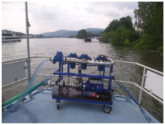
Figure 4.
Portable pressurised pump-filtration system using a filter cascade of 100, 50, and 10 µm filters.
Due to logistical reasons, at the study site in Emmerich, no filter cascade was used. For the first sampling campaign at Koblenz, a smaller filter cascade was used (see Laermanns et al. [50]). Here, the sampling depth was set to the middle of the water column, whereas for the other two filter cascade samples, the sampling depth was approximately 50 cm below the water surface.
2.3. Sample Collection
Four cross-section sampling campaigns were conducted in total: three at Koblenz and one at Emmerich. Campaigns at Koblenz took place on 8 September 2021, 23 November 2021, and 16 March 2023, representing mean-flow conditions (MQ), low discharge (NQ), and flood discharge (HQ), respectively (discharges on the sampling days were 1350, 774, and 2390 m3/s, respectively). The campaign in Emmerich took place on 4 November 2021, during low water conditions with a discharge of 1040 m3/s. Turbidity probes and gravimetrical SSC determination from the nearby suspended sediment monitoring stations of the German Waterways and Shipping Authority recorded mean daily values of 9.8, 9.6, and 55.5 mg/L at Koblenz and 16.5 mg/L at Emmerich. For comparison, the mean annual SSC at Koblenz for 2021 and 2023 were 20 mg/L and 23 mg/L, respectively, and at Emmerich, the mean annual SSC for 2021 was 15 mg/L.
During each campaign, three verticals were sampled along the cross-section, representing the middle, left, and right sections of the river. Sampling positions were located using the GPS of the vessel. Sampling volume and flow velocity within each net were recorded by the flow-meter, yielding mean sampling volumes of 81 m3 at the water surface, 212 m3 in the middle of the water column, and 181 m3 near the riverbed. Mean sampling volumes retrieved by the filter cascade were 3.9 m3 for the particle fractions ≥ 50 µm and 0.6 m3 for the particle fractions 10–50 µm. At each vertical, the sampling duration was set to about one hour to obtain adequate sampling volumes. For each pair of filter nets, samples were not treated as individual samples but pooled into one larger sample per depth.
2.4. Sample Processing and Analysis
Net samples were collected directly on the vessel by back flushing water from the outside of the net, so that the collected material settled into the detachable net cup. This filled cup was then transferred into a clean glass container and covered with aluminium foil. After sampling, the glasses were stored in the dark and cooled until subsequent processing. Also, filter cascade samples, i.e., the filters, were transferred into clean glass containers and covered with aluminium foil and subsequently stored in the dark and cooled.
The collected material was then wet sieved using a sieve tower (Retsch GmbH, Haan, Germany). Fractionation into seven size categories followed, to compare potential gradients among size classes. In principle, particle classification followed the proposed size classes by Bannick et al. [51] to ensure future comparability, but it was extended with two additional classes due to the sampling design using the 300 µm mesh size. Particle classes were therefore set to 10–50 µm, 50–100 µm, 100–300 µm, 300–500 µm, 500 µm–1 mm, 1–5 mm, and 5–25 mm, with the first three originating from fractionated filtration and the latter four stemming from filter nets. Although by definition, the particles > 5 mm are not MPs [52], we included those particles in our study, as particles between 5 and 25 mm can easily degrade over the river course into MPs. Thus, it might be useful for other studies, especially further downstream of our sites, to have information on this size fraction. After fractionation, the samples were freeze-dried. For each fraction, we estimated the dry weight of total sampled suspended matter before further analytical lab procedures.
We followed two established analytical approaches to estimate the polymer masses: Large particles ≥ 1 mm gathered with the filter nets were visually inspected, extracted, and scanned with an ATR FT-IR (Perkin Elmer Inc., Waltham, MA, USA) [53]. Visual inspection was performed directly in the sieves based on physical characteristics of the particles (shape, colour, flotation within the sieve, and texture). Potential MP particles were then cleaned, dried, and transferred into small sample jars using a metal tweezer for further analysis. All particles were then analysed with the ATR FT-IR. An internal database based on additive-free reference materials was used for polymer determination. The following polymers were covered: polyethylene (PE), polypropylene (PP), polystyrene (PS), polyurethane (PU), polyvinyl chloride (PVC), polyamide (PA), polyethylene terephthalate (PET), and polymethylmethacrylate (PMMA). Subsequently, the mass of each polymer category in each size class (1–5 mm and 5–25 mm) was determined by weighting. Each particle was weighted individually. Then, particle weights per polymer category, sample, and size fraction were summed up, resulting in a polymer concentration value per sample and size fraction. All fractions < 1 mm were analysed using pyrolysis gas chromatography coupled with mass spectrometry (pyr-GC-MS) based on Dierkes et al. [54]: Each sample was first extracted via pressurised liquid extraction using methanol (100 °C, 100 bar) for a clean-up step and tetrahydrofuran (185 °C, 100 bar) to extract PE, PP, and PS. All extracts were collected on 200 mg silica gel. After evaporation of the solvent, all silica gel extracts were homogenised and weighed (20.0 mg each) into pyrolysis cups for Pyr-GC-MS analysis (further details for the Pyr-GC-MS measurements are listed in Table S1). For evaluation, polymer masses of PE, PP, and PS were determined (as concentration in mg per g sediment) and for concentration values below the limit of quantification (LOQ), we applied the LOQ of the respective polymer as concentration value (PE: 0.007 mg/g; PP: 0.007 mg/g; PS: 0.008 mg/g). Via sediment mass per sampled volume, the MPs concentration per litre could be determined. In the following sections, all results are given as mass per volume (mg/m3).
2.5. Analysis of MP Concentration (10 µm–25 mm)
For an evaluation of the depth-distribution of MPs, we regarded MP concentrations in mg per m3 water volume for each sampling depth, for each polymer, and for each discharge. We calculated the mean, standard deviation, and minimum and maximum concentration for each size-class and used Kruskal–Wallis tests to evaluate differences in polymer concentration in different categorical classes. To account for variation over the size spectrum excluding depth variation, we then calculated the coefficient of variation for each polymer and each size class over all samples pooled.
2.6. Analysis of Depth-Distribution of MPs (300 µm–25 mm)
All MP concentrations in the size spectrum 300 µm–25 mm were analysed concerning vertical distribution using the Rouse model [55,56]. The Rouse model is used to describe the vertical gradient of suspended sediment concentration based on the dimensionless (Rouse-) number :
where h is the water depth, the height above the channel bed, and the reference concentration at a height above the channel bed. The Rouse number is defined by the ratio of settling velocities of suspended particles () and turbulent mixing forces, expressed by the shear velocity (:
with k as the von Karman constant [15]. Small particles with low Rouse numbers show rather homogeneous distributions, and larger particles with large Rouse numbers represent stronger gradients [15,57]. As the range of settling velocity is considerably larger for MPs than for natural sediment particles due to more heterogeneous densities and particle shapes, a larger spectrum of Rouse profiles is possible for MPs, with low-density rising particles ( < 1 g/cm3) resulting in negative Rouse numbers [10,15,58].
The settling velocity for spherical particles in laminar flow can be calculated based on Stokes’ law [59], using the following formula:
with being the density of the particle, being the density of the fluid, being the gravitational acceleration, and being the dynamic viscosity of the water. describes the particle diameter with the simplification of spherical-shaped particles. Shear velocity for the simplified assumption of uniform flow in wide channels can be derived as follows:
with being the water depth at the regarded site and being the mean river gradient at the regarded site.
We computed Rouse numbers for each analysed polymer using densities of 0.92, 0.94, 1.00, 1.04, 1.14, 1.18, 1.2, and 1.38 g/cm3 for PP, PE, PU, PS, PA, PMMA, PVC, and PET, respectively. As particle diameter, we applied the median of the four size fractions (400 µm, 750 µm, 3 mm, and 15 mm) for the filter net samples.
As an indicator for mixing of MPs in the water column, the ratio of MPs concentration at 10% and 90% above the channel bed was calculated for variable Rouse numbers:
We argue that differences between and should be detectable if < 0.8, given a 20% uncertainty of estimated MP concentrations. For ratios > 0.8, we assumed that turbulent mixing results in a homogenous MPs concentration, and differences of MPs concentration between the top and bottom samples are not detectable. We decided to use 10% and 90% above the channel bed, as those values are close to the uppermost and lowermost sampling depths.
From this theoretical approach, we were able to compare our depth-distributed sampling data and evaluate how accurately the theoretical description of turbulent mixing describes the actual MPs occurrence within the water column of the Rhine River.
Since MPs are frequently sampled at the water surface without considering concentration gradients, we additionally calculated the ratio of the polymer concentration of the uppermost sample and the mean polymer concentration per vertical for each polymer and each grain size fraction > 300 µm. This ratio was taken as an indicator for the vertical mixing of polymers within our samples, with values ~1 indicating vertical mixing, values > 1 indicating higher concentrations towards the water surface, and values <1 indicating higher concentrations at the riverbed.
2.7. Analysis of Lateral and Discharge-Dependent Variability (10 µm–25 mm)
To gain further insights beyond the depth distribution of the MPs concentration, we performed an in-depth analysis of the lateral variability by aggregating samples over the lateral sampling position. Statistical significance of lateral differences was tested with a Kruskal–Wallis test. In addition, an aggregation over the discharge scenarios was performed. Again, a Kruskal–Wallis test was performed for significance inspection.
3. Results and Discussion
3.1. MP Concentration Ranges
Grain size-fractionated concentrations within our samples of the filter nets ranged from no MPs findings (only for the ATR-FTIR analysed samples, i.e., ≥1000 µm) up to 8.08 mg/m3 (total fraction, PP) (Table S2). Fractionated concentrations from filter cascade sampling ranged from 0.0007 mg/m3 (100–300 µm fraction, PP) to 3.303 mg/m3 (100–300 µm fraction, PE) (Table S3). In Figure 5, statistical values (mean, median, and 25% and 75% quantiles) are visualised for each fraction and each sampling campaign, excluding samples without MPs content. Here, a general trend of higher concentration values during the flood event is evident. Single particle findings have a large influence, as indicated by the high mean values in combination with low median values, e.g., apparent for the 100–300 µm fraction during the flood event.
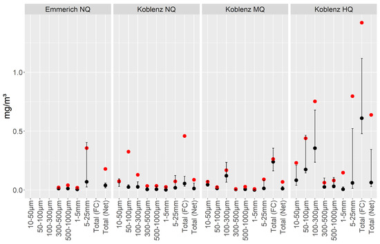
Figure 5.
Statistical overview of the sampled data, aggregated as mean values (red points), median values (black points), and 25% and 75% quantiles (black lines) from all polymer concentration values. Samples without MP content were excluded. Only polymers found are plotted. Data are shown for each size class and each sampling campaign. Values are given as concentration in mg/m3. Data < 1 mm stem from analysis with pyr-GC-MS, and data > 1 mm stem from ATR FT-IR analysis.
To account for the particle size differences within the concentrations and for a differentiation of variability among the polymers, we plotted the coefficient of variation within the cross-section for each size class and each polymer for all samples from the filter nets (each vertical) (Figure 6). A clear trend of increasing variability with increasing grain size is apparent for all polymers. This shows that for all sampling campaigns, smaller MP particles are more homogenously distributed than larger MP particles over (i) sampling position and (ii) discharge scenario. Additionally, in the larger fractions, a polymer was often found in only one depth, resulting in a similar coefficient of variation, regardless of the concentration of the polymer found (e.g., PE in the 5–25 mm fraction).
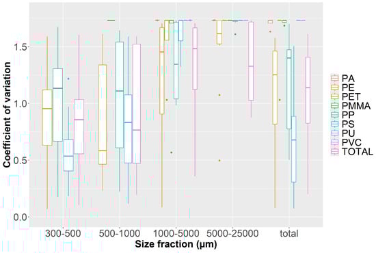
Figure 6.
Boxplots of the coefficients of variation from all filter net samples (all water depths and all four campaigns) as a measure of dimensionless variation of MP concentrations over the size fractions regarded. Data < 1 mm stem from analysis with pyr-GC-MS, and data > 1 mm stem from ATR FT-IR analysis. Dots represent outlier values with at least a 1.5-fold interquartile range above the 3rd or below the 1st quartile.
3.2. Vertical Gradients
MPs sampled at three depths show no consistent vertical trend of concentrations for various polymers (Figure 7). Most concentration values are very low, and only a few higher concentrations stand out. PE, PP, and PS show a higher number of findings, which can be partially attributed to the additional analysis method for the three smaller size classes for those polymers, contributing to a higher number of points in Figure 7. A trend of higher MP concentrations at the water surface and during HQ can be seen. In general, the picture seems to be complex, as most polymers are found in each depth and during each discharge scenario (for fractionated concentration profiles, see Figures S1–S4). Samples stemming from the filter cascade are in a comparable concentration range as those derived from the filter nets, with a few higher concentrations detected (e.g., PE during the flood campaign (5.05 mg/m3) and PS during the Koblenz NQ campaign (1.96 mg/m3)). This is in accordance with the values in Tables S2 and S3.
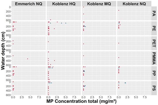
Figure 7.
Total MP concentrations (mg/m3) per water depth (cm), including all size fractions of all four campaigns. Blue triangles mark the samples obtained from the filter cascade, and red points are filter net samples. Samples without MPs content were excluded. Only polymers found are plotted. Data stem from both analysis via pyr-GC-MS and ATR FT-IR analysis.
Expected MPs concentration ratios at 10% and 90% above the channel bed derived from idealised Rouse profiles for different Rouse numbers are plotted in Figure 8. Here, we assumed that a ratio of > 0.8 is related to well-mixed conditions, which can be hardly detected using uncertainties of estimated MP concentrations larger than 20%. For the smallest size classes (400 µm and 750 µm), calculated Rouse numbers for the considered polymers are typically smaller, implying that is closer to one. Thus, differences between bottom and surface concentrations are hardly predicted considering combined sampling/analytical uncertainties > 20%. However, MP particles > 3 mm have Rouse numbers resulting in strong gradients and < 0.8, indicative of strong differences between top and bottom samples. These results are only partly congruent with our in situ data in Figure 7: although slight gradients can be observed with a few larger concentration values near the water surface for PE and PP, in general, particles are found throughout the whole water column.
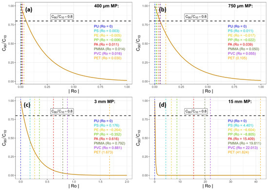
Figure 8.
Calculated Rouse numbers for all polymers regarded in this study and the respective ratio of turbulent mixing for each Rouse number: a concentration ratio of 10% and 90% above the river bed was regarded. The dotted horizontal line represents a ratio of 0.8, specified here as a threshold where a uniform concentration distribution is probable. Rouse numbers (dotted vertical lines) intersecting this line within the concentration ratio curves thus represent uniform MP concentrations within the water column, whereas Rouse numbers not intersecting the line represent concentration gradients within the water column. For PE and PP, Rouse numbers are negative due to their densities being lower than water. Thus, the ratio would be C2/C1 instead, meaning that for values < 1, the concentration near the water surface is higher than with increasing water depth. Subfigures (a–d) represent the median of our four size fractions (400 µm, 750 µm, 3 mm and 15 mm) respectively.
Figure 9 and Figure 10 show the ratio of the MPs concentration of the uppermost sample and the mean of all samples per vertical. Boxes include samples from all campaigns, separated by polymer type and particle size.
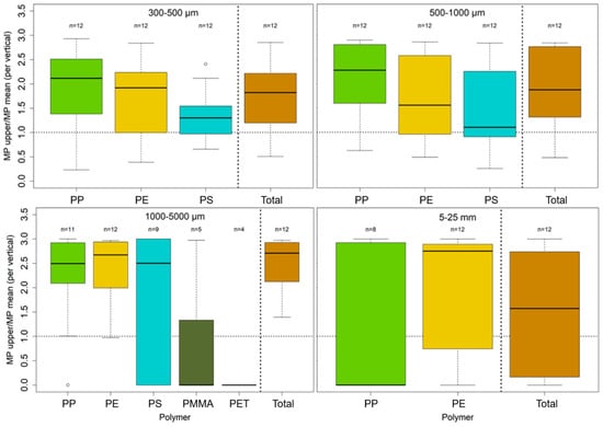
Figure 9.
Boxplot of the ratios of upper MPs concentration close to the water surface and mean concentration per vertical for each polymer and each size fraction. Dotted horizontal lines mark a ratio of 1, where the upper MPs concentration and the mean of the vertical are similar; values above represent higher concentrations at the water surface and vice versa. Unfilled dots represent outlier values with at least a 1.5-fold interquartile range above the 3rd or below the 1st quartile. Only values with n > 3 were plotted, meaning that data from at least three verticals were available for ratio calculation. The polymers on the x-axis are sorted by means of density in an ascending order from PP (0.92 g/cm3) to PET (1.38 g/cm3). Data < 1 mm stem from analysis with pyr-GC-MS, and data > 1 mm stem from ATR FT-IR analysis.
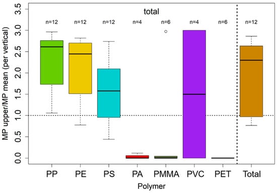
Figure 10.
Boxplot of the ratios of upper MPs concentration and mean MPs concentration per vertical for each polymer for the total fraction, aggregated over all size fractions. Dotted horizontal lines mark a ratio of 1, where the upper MPs concentration and the mean of the vertical are similar; values above represent higher concentrations at the water surface and vice versa. Unfilled dots represent outlier values with at least a 1.5-fold interquartile range above the 3rd or below the 1st quartile. Only values with n > 3 were plotted, meaning that data from at least three verticals were available for ratio calculation. The polymers on the x-axis are sorted by means of density in an ascending order from PP (0.92 g/cm3) to PET (1.38 g/cm3). Data stem from both analysis via pyr-GC-MS and ATR FT-IR analysis.
Except for a few cases, MP concentrations at the surface are higher than profile average concentrations. In general, PP with the lowest density (0.92 g/cm3) shows the highest surface/depth-average ratio, followed, in order and by polymer density, by PE and PS (0.94 g/cm3 and 1.04 g/cm3). For PP and PE, concentrations are 2 to 2.5-fold higher at the surface compared to the whole water column. For PA and PMMA, which both have densities > 1 g/cm3 (1.14 g/cm3 and 1.18 g/cm3), the ratio is smaller than one, indicating reduced surface concentrations. However, sample numbers of these polymers are relatively low, and results have to be treated with care. This is also true for particle sizes > 5 mm, which show strongly scattering concentrations that are strongly affected by single particles. In this context, the surface/depth-average ratio for PP for large particles strongly deviates from the results for particles < 5 mm.
From this comparison of theoretical approaches and sampling data (Figure 8 and Figure 9), it becomes clear that, opposed to the theoretical calculation using Rouse’s theory, vertical gradients seem to be pronounced even in smaller size classes. Possible explanations are the discrepancies between idealised raw-polymer densities and the more complex properties of MPs occurring in the environment, as many studies have shown pronounced effects of biofilm accumulation and weathering on both rising and settling velocities of MPs [58,60,61]. Although effects are complex and dependent on particle shape, an increase in the respective velocity is often described. In addition, it has been shown that especially small MPs < 162 µm tend to be incorporated into heteroaggregates [62,63], altering the effective grainsize and thus settling velocity during transport (see Equation (3)), leading to more pronounced gradients. Also, particle shapes of MPs are often far from round (which is the underlying theory of the theoretical approach), again altering settling and rising velocities [58,64,65].
3.3. Lateral and Discharge-Dependent Variability
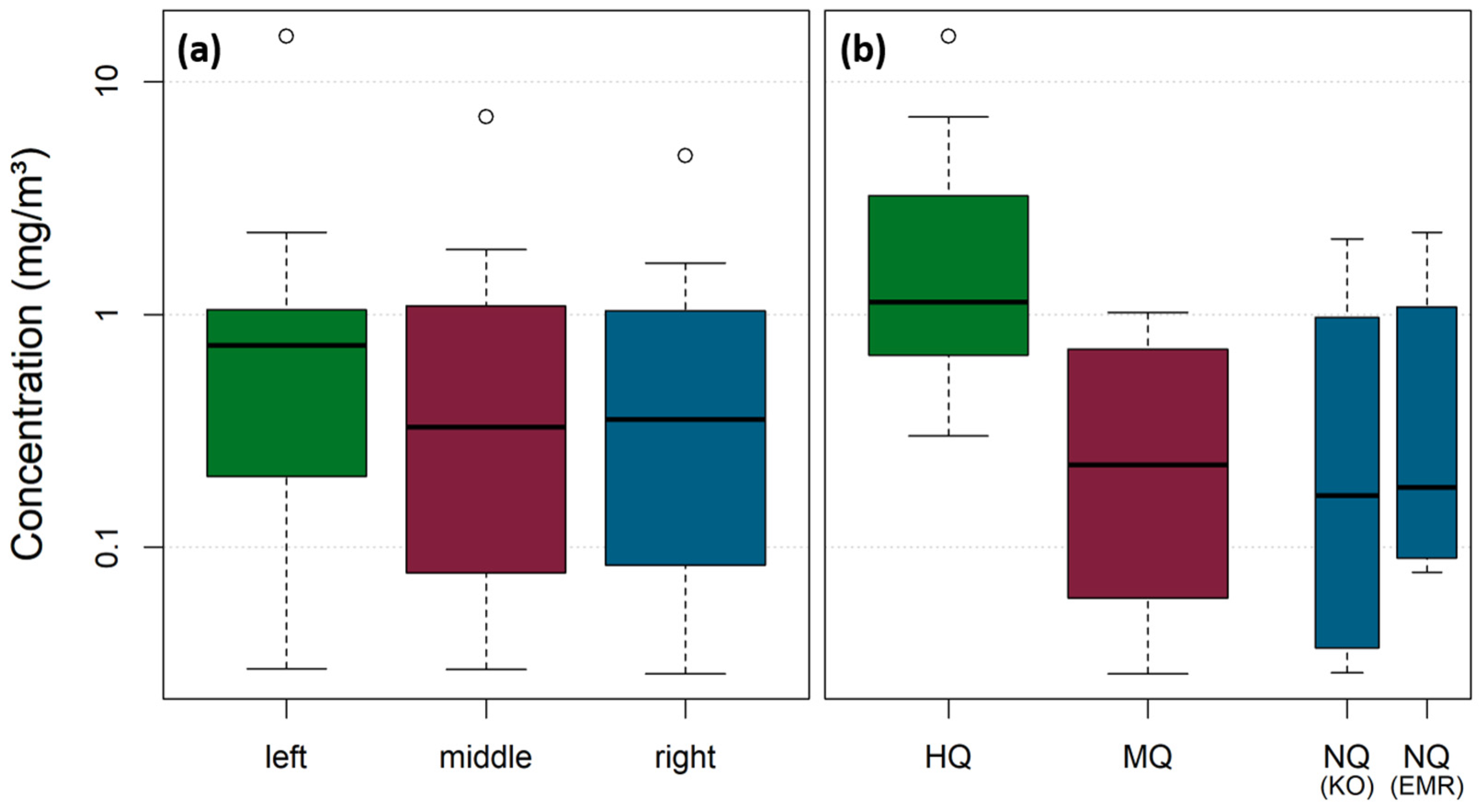
For samples stemming from the left river sides of the Rhine, marginally higher MP concentrations are apparent (median: 0.74 mg/m3), whereas middle and right samples are in a similar range (median: 0.33 mg/m3 and 0.35 mg/m3) (Figure 11a). These differences are not statistically significant with a significance level of 0.05 (Kruskal–Wallis Test, p-value = 0.73). However, during HQ, the MP concentrations increased significantly (median and standard error: 1.13 ± 1.30 mg/m3) compared to MQ (median and standard error: 0.23 ± 0.11 mg/m3) and NQ campaigns (Figure 11b). MP concentrations for both Koblenz (median and standard error: 0.17 ± 0.22 mg/m3) and Emmerich (median and standard error: 0.18 ± 0.25 mg/m3) were in a comparable range during NQ. The differences among the varying discharges are statistically significant with a significance level of 0.05 (Kruskal–Wallis Test, p-value = 0.006). An additional Wilcoxon test reveals that the differences between HQ-MQ and HQ-NQ are statistically significant (p = 0.004 and p = 0.02), whereas the differences between MQ and NQ are not statistically significant (p = 0.98).
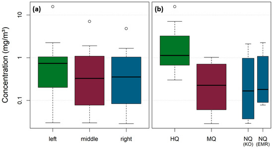
Figure 11.
Total concentration values of all filter net and cascade samplings in mg/m3 differentiated between lateral sampling position (left/middle/right) (a) and differentiated between discharge scenario (HQ/MQ/NQ) (b). For NQ campaigns, both Koblenz and Emmerich were plotted as separate boxes. The y-axis is plotted log-scaled for better visualization. Data stem from both analysis via pyr-GC-MS and ATR FT-IR analysis.
Both sampling sites are not located within strongly curved meanders. The Lahn River enters the Rhine River 4.3 km upstream of the sampling site in Koblenz, on the right river side (at Rhine km 585.7). As the Lahn River only contributes about 3% to the discharge of the Rhine at Koblenz, it is unlikely that the slightly higher MP concentrations from the left verticals over all campaigns and sites originate from diluting effects from the Lahn River, and they are rather random variations. This is underlined by the fact that no statistical significance could be detected among the lateral position (significance level of 0.05 (Kruskal–Wallis Test, p-value = 0.73)).
As expected from the literature and from Figure S5, MP concentrations during flood events are increased [7,12,14,26,36,41,46,66,67,68,69,70,71]. MP concentrations during low discharge conditions and during mean discharge conditions are in a comparable range in our study. In Emmerich, only net sampling was applied, influencing the NQ concentration because the share of larger MP particles for NQ is higher compared to the other campaigns, where a combination of net sampling and filter cascade sampling was applied. Larger particles occur less frequently but have a higher impact on the concentration due to their higher weight (see Table S4). Emmerich is situated downstream the Ruhr area (Rhine km 852) and 269 km downstream of the sampling site in Koblenz, and therefore, concentrations in Emmerich are likely to be higher than in Koblenz, as previously shown by Mani et al. [39]. When considering the SSC of the respective NQ and MQ sampling days, it can be seen that the turbidity values also were within a similar range (NQ: 9.6 mg/L, MQ: 9.8 mg/L), which implies that the suspended matter concentration in general might increase not before a distinct threshold, or more specific, that rating coefficients vary over the discharge range. This has been shown previously by Hoffmann et al. [45] and is supported for MP concentrations at Koblenz by Range et al. [72].
3.4. Limitations
During the sampling campaigns, shipping traffic was present, causing waves. In addition to strong turbulences due to the high flow velocities, it was difficult to keep the uppermost nets in a constant water depth at the surface despite the floating bodies mounted at the uppermost filter nets. This might have affected the flow-meters, which are positioned in the middle of the net openings: water may have entered the nets without the flow-meters measuring the volume correctly. This means that the uppermost sampling volumes are possibly slightly underestimated, and that the concentration values are possibly slightly overestimated with regard to the sampling volume. Another drawback inherent to the filter nets is a possible loss of fibres and other elongated particle forms, which may pass the mesh, resulting in a possible underestimation of the MP concentrations [31]. MP particles > 1 mm were removed by visual inspection of the sample. Due to a risk of missing MP particles, an underestimation of selected MP particles cannot be ruled out. For our theoretical approach to describe the depth distribution of the polymers, it has to be kept in mind that we used mean polymer density values. MP particles that occur in the environment are often characterised by different degrees of degradation or a combination with additives, resulting in a wide range of occurring densities [73]. This has not been covered in the calculated depth profiles, as knowledge about the density of MP particles in the environment is very limited and has not been estimated in this study. Despite the drawbacks, our study is a pilot study and, thus, it can serve as a basis for potential future MPs flux monitoring in large river systems. Still, future cross-sectional sampling campaigns need to address the problem of determining the correct sampling volume, either by additional flow velocity measurements or by reducing the height of the uppermost sample, so that a constant submergence can be guaranteed.
3.5. Implications
Our study is the first in the Rhine River performing multiple depth-distributed sampling campaigns to gather insights into the cross-sectional variability of MPs on mass-based analysis. As previous studies regarded particle counts instead of concentrations based on mass, a comparison to other studies within the Rhine River catchment is limited (Table 1). Nevertheless, our results show that in the Rhine River, at Koblenz and Emmerich, MPs occur over the whole water depth and can thus be considered ubiquitously distributed contaminants.
Cowger et al. [15] differentiated two common approaches in the literature regarding how conclusions from surface sampling are drawn: the surface load assumption, where a surface-only occurrence of MPs is assumed, and the wash load assumption, where a uniformly distributed MP concentration within the cross-section is assumed. Our results show that both approaches failed at our sampling sites, with the first approach leading to underestimations because of the neglect of MP particles below the water surface, and the second approach leading to overestimations for low-density and underestimations for high-density MPs because of diverging concentrations with increasing water depth.
Although we confirmed the outcome of a previous study showing that high discharge events result in higher MPs fluxes, MPs are constantly carried within the water column [72], also during mean and even low discharges. This constant flux inevitably implicates high MP loads, which ultimately enter the North Sea.
4. Conclusions
Within our study, we built two innovative sampling devices to gather insights into the cross-sectional variability of MPs in the Rhine River. As the first study applying depth-distributed and spatially high-resolution MPs sampling in the Rhine River, we were able to show that MPs can be considered as ubiquitous pollutants in Europe’s busiest waterway. Although we expected concentration depth profiles for different polymers within the water column due to theoretical calculations, we identified that the field data show a more complex image. At first glance, polymers seemed to be mixed over the whole water column, probably due to turbulent flow within the river. With the ratio of upper concentration against mean concentration per vertical, we could reveal that density seems to be more decisive for the vertical position of small MPs than expected from theory: even smaller particles’ ratio was sorted by the polymer density, with high ratios for light polymers and vice versa. This, in turn, verifies our hypothesis that sampling without including spatiotemporal knowledge may lead to errors, no matter whether a surface load assumption or a wash load assumption is assumed. On the basis of the coefficient of variation for the size fractions, we showed that for increasing particle size, variation within the river becomes more likely, which indicates that larger sampling volumes are needed. These aspects highlight the difficulty of acquiring representative data for larger MP particles both spatially and temporally.
No statistically significant lateral variations have been detected. For the respective discharge scenarios, it has been shown that a clear trend to higher MP concentrations is apparent during HQ events, and that MQ and NQ scenarios do not differ greatly. This is in agreement with findings in the literature.
On the basis of our findings, we suggest that MPs sampling within the Rhine River ideally is adapted to the addressed interest: If large MP particles are of interest, sampling techniques like filter nets are helpful, because they effectively sample large water volumes in a short period of time and can be adapted at different water depths. Smaller particles can be sampled more easily, e.g., with pump setups. Depending on specific questioning, spot tests might be sufficient; still, depth-distributed sampling seems to be the best practice for precise MP concentration determinations within river cross-sections. For sampling the whole spectrum of MP sizes, now, as before, a combination of different sampling methods seems to be promising in the future. On the basis of this study, being this the first one to comprehensively regard cross-sectional aspects during sampling and to address MP masses as a more robust unit in terms of MP quantification rather than item numbers in the Rhine River, we lay a foundation for future research and monitoring in this catchment: we could demonstrate that the sampling position and the sampling time do have an impact on the representativity of the sample, although MPs do occur ubiquitously in the Rhine River. Thus, with this study, we provide information for future sampling campaigns in terms of sampling design and even for potential future monitoring programmes in the Rhine River.
Supplementary Materials
The following supporting information can be downloaded at: https://www.mdpi.com/article/10.3390/microplastics4020027/s1, Figure S1: Plastic concentration within the water depth for the size fraction 5–25 mm for the polymers PA, PE, PMMA, PP, PS, PU and PVC; Figure S2: Plastic concentration within the water depth for the size fraction 1–5 mm for the polymers PA, PE, PMMA, PP, PS, PU, and PVC; Figure S3: Plastic concentration within the water depth for the size fraction 500–1000 µm for the polymers PA, PE, PMMA, PP, PS, PU, and PVC; Figure S4: Plastic concentration within the water depth for the size fraction 300–500 µm for the polymers PA, PE, PMMA, PP, PS, PU, and PVC; Figure S5: Lateral variation of MP concentrations and variation of MPs with discharge scenarios. Only Koblenz campaigns were taken for this plot; Table S1: Mean MP concentrations of all captured particle size classes over all sampling campaigns; Table S2: Statistical overview of MPs sampling data from the filter nets during the four sampling campaigns, both for each size fraction and for the total size fraction aggregated over all four size classes. Values are given as concentration in mg/m3, and values in brackets represent the standard deviation; Table S3: Statistical overview of MPs sampling data from the filter cascade during the three sampling campaigns, both for each size fraction and for the total size fraction aggregated over all three size classes. Values are given as concentration in mg/m3, and values in brackets represent the standard deviation; Table S4: Experimental parameters and instrumental parts of the Py-GC-MS system.
Author Contributions
Conceptualization, D.R. and T.H.; methodology, D.R., J.K. and G.D.; investigation, D.R.; data curation, D.R.; writing—original draft preparation, D.R.; writing—review and editing, D.R., J.K., G.D., T.T. and T.H.; visualization, D.R.; supervision, T.H.; project administration, T.T. All authors have read and agreed to the published version of the manuscript.
Funding
This study was part of the project ‘Monitoring and Budgeting of microplastics in the Rhine River’, which was funded by the German Environment Agency (Umweltbundesamt, Forschungskennzahl 3719 22 301 0). The authors are grateful to the Federal Ministry for Digital and Transport (BMDV) for their financial support.
Institutional Review Board Statement
Not applicable.
Informed Consent Statement
Not applicable.
Data Availability Statement
Dataset available upon request from the authors.
Acknowledgments
Authors would like to thank both reviewers for their constructive comments. Furthermore, authors would like to thank the WSV for the possibility to use the vessels during the sampling campaigns.
Conflicts of Interest
The authors declare no conflicts of interest.
Abbreviations
The following abbreviations are used in this manuscript:
| MP | microplastic |
| PE | Polyethylene |
| PP | Polypropylene |
| PS | Polystyrene |
| PMMA | Polymethylmethacrylate |
| PA | Polyamide |
| PU | Polyurethane |
| PVC | Polyvinyl chloride |
| PET | Polyethylene terepthalate |
| NQ | Low discharge |
| MQ | Mean-flow |
| HQ | Flood discharge |
| Pyr-GC-MS | Pyrolysis gas chromatography coupled with mass spectrometry |
References
- Wang, Z.; Zhang, Y.; Kang, S.; Yang, L.; Shi, H.; Tripathee, L.; Gao, T. Research progresses of microplastic pollution in freshwater systems. Sci. Total Environ. 2021, 795, 148888. [Google Scholar] [CrossRef] [PubMed]
- Petersen, F.; Hubbart, J.A. The occurrence and transport of microplastics: The state of the science. Sci. Total Environ. 2021, 758, 143936. [Google Scholar] [CrossRef]
- Kumar, R.; Sharma, P.; Verma, A.; Jha, P.K.; Singh, P.; Gupta, P.K.; Chandra, R.; Prasad, P.V.V. Effect of Physical Characteristics and Hydrodynamic Conditions on Transport and Deposition of Microplastics in Riverine Ecosystem. Water 2021, 13, 2710. [Google Scholar] [CrossRef]
- Wagner, M.; Scherer, C.; Alvarez-Munoz, D.; Brennholt, N.; Bourrain, X.; Buchinger, S.; Fries, E.; Grosbois, C.; Klasmeier, J.; Marti, T.; et al. Microplastics in freshwater ecosystems: What we know and what we need to know. Environ. Sci. Eur. 2014, 26, 12. [Google Scholar] [CrossRef]
- Hamm, T.; Lorenz, C.; Piehl, S. Microplastics in Aquatic Systems—Monitoring Methods and Biological Consequences; Springer: Cham, Switzerland, 2018; pp. 179–195. [Google Scholar]
- Frei, S.; Piehl, S.; Gilfedder, B.S.; Loder, M.G.J.; Krutzke, J.; Wilhelm, L.; Laforsch, C. Occurence of microplastics in the hyporheic zone of rivers. Sci. Rep. 2019, 9, 15256. [Google Scholar] [CrossRef]
- Rodrigues, S.M.; Almeida, C.M.R.; Silva, D.; Cunha, J.; Antunes, C.; Freitas, V.; Ramos, S. Microplastic contamination in an urban estuary: Abundance and distribution of microplastics and fish larvae in the Douro estuary. Sci. Total Environ. 2019, 659, 1071–1081. [Google Scholar] [CrossRef]
- Yan, M.; Wang, L.; Dai, Y.; Sun, H.; Liu, C. Behavior of Microplastics in Inland Waters: Aggregation, Settlement, and Transport. Bull. Environ. Contam. Toxicol. 2021, 107, 700–709. [Google Scholar] [CrossRef]
- Talbot, R.; Chang, H. Microplastics in freshwater: A global review of factors affecting spatial and temporal variations. Environ. Pollut. 2022, 292, 118393. [Google Scholar] [CrossRef]
- Waldschläger, K.; Brückner, M.Z.M.; Carney Almroth, B.; Hackney, C.R.; Adyel, T.M.; Alimi, O.S.; Belontz, S.L.; Cowger, W.; Doyle, D.; Gray, A.; et al. Learning from natural sediments to tackle microplastics challenges: A multidisciplinary perspective. Earth-Sci. Rev. 2022, 228. [Google Scholar] [CrossRef]
- Bai, M.; Lin, Y.; Hurley, R.R.; Zhu, L.; Li, D. Controlling Factors of Microplastic Riverine Flux and Implications for Reliable Monitoring Strategy. Environ. Sci. Technol. 2022, 56, 48–61. [Google Scholar] [CrossRef]
- de Carvalho, A.R.; Riem-Galliano, L.; Ter Halle, A.; Cucherousset, J. Interactive effect of urbanization and flood in modulating microplastic pollution in rivers. Environ. Pollut. 2022, 309, 119760. [Google Scholar] [CrossRef]
- Pessenlehner, S.; Gmeiner, P.; Habersack, H.; Liedermann, M. Understanding the spatio-temporal behaviour of riverine plastic transport and its significance for flux determination: Insights from direct measurements in the Austrian Danube River. Front. Earth Sci. 2024, 12, 1426158. [Google Scholar] [CrossRef]
- Eo, S.; Hong, S.H.; Song, Y.K.; Han, G.M.; Shim, W.J. Spatiotemporal distribution and annual load of microplastics in the Nakdong River, South Korea. Water Res. 2019, 160, 228–237. [Google Scholar] [CrossRef]
- Cowger, W.; Gray, A.B.; Guilinger, J.J.; Fong, B.; Waldschlager, K. Concentration Depth Profiles of Microplastic Particles in River Flow and Implications for Surface Sampling. Environ. Sci. Technol. 2021, 55, 6032–6041. [Google Scholar] [CrossRef]
- Kiss, T.; Gönczy, S.; Nagy, T.; Mesaroš, M.; Balla, A. Deposition and Mobilization of Microplastics in a Low-Energy Fluvial Environment from a Geomorphological Perspective. Appl. Sci. 2022, 12, 4367. [Google Scholar] [CrossRef]
- Range, D.; Scherer, C.; Stock, F.; Ternes, T.A.; Hoffmann, T.O. Hydro-geomorphic perspectives on microplastic distribution in freshwater river systems: A critical review. Water Res. 2023, 245, 120567. [Google Scholar] [CrossRef]
- Slabon, A.; Terweh, S.; Hoffmann, T.O. Vertical and Lateral Variability of Suspended Sediment Transport in the Rhine River. Hydrol. Process. 2025, 39, e70070. [Google Scholar] [CrossRef]
- Slabon, A.; Hoffmann, T. Vertical and lateral variability of suspended sediment in crosssections at the river Rhine. In Proceedings of the EGU General Assembly 2022, Vienna, Austria, 23–27 May 2022. [Google Scholar]
- Liedermann, M.; Gmeiner, P.; Pessenlehner, S.; Haimann, M.; Hohenblum, P.; Habersack, H. A Methodology for Measuring Microplastic Transport in Large or Medium Rivers. Water 2018, 10, 414. [Google Scholar] [CrossRef]
- Lenaker, P.L.; Baldwin, A.K.; Corsi, S.R.; Mason, S.A.; Reneau, P.C.; Scott, J.W. Vertical Distribution of Microplastics in the Water Column and Surficial Sediment from the Milwaukee River Basin to Lake Michigan. Environ. Sci. Technol. 2019, 53, 12227–12237. [Google Scholar] [CrossRef]
- Pasquier, G.; Doyen, P.; Dehaut, A.; Veillet, G.; Duflos, G.; Amara, R. Vertical distribution of microplastics in a river water column using an innovative sampling method. Environ. Monit. Assess. 2023, 195, 1302. [Google Scholar] [CrossRef]
- Procop, I.; Calmuc, M.; Pessenlehner, S.; Trifu, C.; Ceoromila, A.C.; Calmuc, V.A.; Fetecău, C.; Iticescu, C.; Musat, V.; Liedermann, M. The first spatio-temporal study of the microplastics and meso–macroplastics transport in the Romanian Danube. Environ. Sci. Eur. 2024, 36, 154. [Google Scholar] [CrossRef]
- Miao, L.; Gao, Y.; Adyel, T.M.; Huo, Z.; Liu, Z.; Wu, J.; Hou, J. Effects of biofilm colonization on the sinking of microplastics in three freshwater environments. J. Hazard. Mater. 2021, 413, 125370. [Google Scholar] [CrossRef]
- Andrady, A.L. Microplastics in the marine environment. Mar. Pollut. Bull. 2011, 62, 1596–1605. [Google Scholar] [CrossRef]
- Haberstroh, C.J.; Arias, M.E.; Yin, Z.; Wang, M.C. Effects of hydrodynamics on the cross-sectional distribution and transport of plastic in an urban coastal river. Water Environ. Res. 2021, 93, 186–200. [Google Scholar] [CrossRef]
- Gitto, A.B.; Venditti, J.G.; Kostaschuk, R.; Church, M. Representative point-integrated suspended sediment sampling in rivers. Water Resour. Res. 2017, 53, 2956–2971. [Google Scholar] [CrossRef]
- Liu, Y.; You, J.; Li, Y.; Zhang, J.; He, Y.; Breider, F.; Tao, S.; Liu, W. Insights into the horizontal and vertical profiles of microplastics in a river emptying into the sea affected by intensive anthropogenic activities in Northern China. Sci. Total Environ. 2021, 779, 146589. [Google Scholar] [CrossRef]
- Rodrigues, M.O.; Abrantes, N.; Goncalves, F.J.M.; Nogueira, H.; Marques, J.C.; Goncalves, A.M.M. Spatial and temporal distribution of microplastics in water and sediments of a freshwater system (Antua River, Portugal). Sci. Total Environ. 2018, 633, 1549–1559. [Google Scholar] [CrossRef]
- Koelmans, A.A.; Mohamed Nor, N.H.; Hermsen, E.; Kooi, M.; Mintenig, S.M.; De France, J. Microplastics in freshwaters and drinking water: Critical review and assessment of data quality. Water Res. 2019, 155, 410–422. [Google Scholar] [CrossRef]
- Campanale, C.; Savino, I.; Pojar, I.; Massarelli, C.; Uricchio, V.F. A Practical Overview of Methodologies for Sampling and Analysis of Microplastics in Riverine Environments. Sustainability 2020, 12, 6755. [Google Scholar] [CrossRef]
- Lu, H.-C.; Ziajahromi, S.; Neale, P.A.; Leusch, F.D.L. A systematic review of freshwater microplastics in water and sediments: Recommendations for harmonisation to enhance future study comparisons. Sci. Total Environ. 2021, 781, 146693. [Google Scholar] [CrossRef]
- Lebreton, L.C.M.; van der Zwet, J.; Damsteeg, J.W.; Slat, B.; Andrady, A.; Reisser, J. River plastic emissions to the world’s oceans. Nat. Commun. 2017, 8, 15611. [Google Scholar] [CrossRef] [PubMed]
- Kataoka, T.; Nihei, Y.; Kudou, K.; Hinata, H. Assessment of the sources and inflow processes of microplastics in the river environments of Japan. Environ. Pollut. 2019, 244, 958–965. [Google Scholar] [CrossRef]
- Whitehead, P.G.; Bussi, G.; Hughes, J.M.R.; Castro-Castellon, A.T.; Norling, M.D.; Jeffers, E.S.; Rampley, C.P.N.; Read, D.S.; Horton, A.A. Modelling Microplastics in the River Thames: Sources, Sinks and Policy Implications. Water 2021, 13, 861. [Google Scholar] [CrossRef]
- Schell, T.; Hurley, R.; Nizzetto, L.; Rico, A.; Vighi, M. Spatio-temporal distribution of microplastics in a Mediterranean river catchment: The importance of wastewater as an environmental pathway. J. Hazard. Mater. 2021, 420, 126481. [Google Scholar] [CrossRef]
- Simon, M.; van Alst, N.; Vollertsen, J. Quantification of microplastic mass and removal rates at wastewater treatment plants applying Focal Plane Array (FPA)-based Fourier Transform Infrared (FT-IR) imaging. Water Res. 2018, 142, 1–9. [Google Scholar] [CrossRef]
- Heß, M.; Diehl, P.; Mayer, J.; Rahm, H.; Reifenhäuser, W.; Stark, J.; Schwaiger, J.J.B.-ü.U.i.B.-W. Bayern, Hessen, Nordrhein-Westfalen und Rheinland-Pfalz. Teil. Mikroplastik in Binnengewässern Süd-und Westdeutschlands. Project Rep. 2018, 1, 84. Available online: https://www.lanuk.nrw.de/fileadmin/lanuvpubl/6_sonderreihen/L%c3%a4nderbericht_Mikroplastik_in_Binnengew%c3%a4ssern.pdf (accessed on 4 May 2025).
- Mani, T.; Hauk, A.; Walter, U.; Burkhardt-Holm, P. Microplastics profile along the Rhine River. Sci. Rep. 2015, 5, 17988. [Google Scholar] [CrossRef]
- Mani, T.; Blarer, P.; Storck, F.R.; Pittroff, M.; Wernicke, T.; Burkhardt-Holm, P. Repeated detection of polystyrene microbeads in the Lower Rhine River. Environ. Pollut. 2019, 245, 634–641. [Google Scholar] [CrossRef]
- Mani, T.; Burkhardt-Holm, P. Seasonal microplastics variation in nival and pluvial stretches of the Rhine River - From the Swiss catchment towards the North Sea. Sci. Total Environ. 2020, 707, 135579. [Google Scholar] [CrossRef]
- Schrank, I.; Löder, M.G.J.; Imhof, H.K.; Moses, S.R.; Heß, M.; Schwaiger, J.; Laforsch, C. Riverine microplastic contamination in southwest Germany: A large-scale survey. Front. Earth Sci. 2022, 10. [Google Scholar] [CrossRef]
- Schwandt, D.; Hübner, G. Informationsplattform Undine. Available online: https://undine.bafg.de/rhein/rheingebiet.html (accessed on 7 February 2022).
- Ministry of Environment, A. Conservation and Consumer Protection, State of North Rhine-Westphalia Flussgebiete NRW. Available online: https://www.flussgebiete.nrw.de/ (accessed on 15 January 2025).
- Hoffmann, T.O.; Baulig, Y.; Fischer, H.; Blöthe, J. Scale breaks of suspended sediment rating in large rivers in Germany induced by organic matter. Earth Surf. Dyn. 2020, 8, 661–678. [Google Scholar] [CrossRef]
- Campanale, C.; Stock, F.; Massarelli, C.; Kochleus, C.; Bagnuolo, G.; Reifferscheid, G.; Uricchio, V.F. Microplastics and their possible sources: The example of Ofanto river in southeast Italy. Environ. Pollut. 2020, 258, 113284. [Google Scholar] [CrossRef] [PubMed]
- Hernroth, L. Sampling and filtration efficiency of two commonly used plankton nets. A comparative study of the Nansen net and the Unesco WP 2 net. J. Plankton Res. 1987, 9, 719–728. [Google Scholar] [CrossRef]
- Smith, P.E.; Counts, R.C.; Clutter, R.I. Changes in Filtering Efficiency of Plankton Nets Due to Clogging Under Tow. ICES J. Mar. Sci. 1968, 32, 232–248. [Google Scholar] [CrossRef]
- Khatmullina, L.; Isachenko, I. Settling velocity of microplastic particles of regular shapes. Mar. Pollut. Bull. 2017, 114, 871–880. [Google Scholar] [CrossRef]
- Laermanns, H.; Reifferscheid, G.; Kruse, J.; Földi, C.; Dierkes, G.; Schaefer, D.; Scherer, C.; Bogner, C.; Stock, F. Microplastic in Water and Sediments at the Confluence of the Elbe and Mulde Rivers in Germany. Front. Environ. Sci. 2021, 9, 794895. [Google Scholar] [CrossRef]
- Bannick, C.G.; Szewzyk, R.; Ricking, M.; Schniegler, S.; Obermaier, N.; Barthel, A.K.; Altmann, K.; Eisentraut, P.; Braun, U. Development and testing of a fractionated filtration for sampling of microplastics in water. Water Res. 2019, 149, 650–658. [Google Scholar] [CrossRef]
- Arthur, C.; Baker, J.; Bamford, H. Proceedings of the International Research Workshop on the Occurrence, Effects, and Fate of Microplastic Marine Debris. In Proceedings of the NOAA Technical Memorandum NOS-OR&R-30, Tacoma, WA, USA, 9–11 September 2008. [Google Scholar]
- Xu, J.-L.; Thomas, K.V.; Luo, Z.; Gowen, A.A. FTIR and Raman imaging for microplastics analysis: State of the art, challenges and prospects. TrAC Trends Anal. Chem. 2019, 119, 115629. [Google Scholar] [CrossRef]
- Dierkes, G.; Lauschke, T.; Becher, S.; Schumacher, H.; Foldi, C.; Ternes, T. Quantification of microplastics in environmental samples via pressurized liquid extraction and pyrolysis-gas chromatography. Anal. Bioanal. Chem. 2019, 411, 6959–6968. [Google Scholar] [CrossRef]
- Bouchez, J.; Métivier, F.; Lupker, M.; Maurice, L.; Perez, M.; Gaillardet, J.; France-Lanord, C. Prediction of depth-integrated fluxes of suspended sediment in the Amazon River: Particle aggregation as a complicating factor. Hydrol. Process. 2010, 25, 778–794. [Google Scholar] [CrossRef]
- Rouse, H. Modern Conceptions of the Mechanics of Fluid Turbulence. Trans. Am. Soc. Civil. Eng. 1937, 102, 463–505. [Google Scholar] [CrossRef]
- Naden, P.S. The Fine-Sediment Cascade. In Sediment Cascades; Burt, T.P., Allison, R.J., Eds.; John Wiley & Sons Ltd.: Hoboken, NJ, USA, 2010; pp. 271–305. [Google Scholar]
- Waldschläger, K.; Born, M.; Cowger, W.; Gray, A.; Schüttrumpf, H. Settling and rising velocities of environmentally weathered micro- and macroplastic particles. Environ. Res. 2020, 191, 110192. [Google Scholar] [CrossRef]
- Stokes, G.G. On the Effect of the Internal Friction of Fluids on the Motion of Pendulum. Pitt. Press. 1851, 9. [Google Scholar] [CrossRef]
- Mendrik, F.; Fernández, R.; Hackney, C.R.; Waller, C.; Parsons, D.R. Non-buoyant microplastic settling velocity varies with biofilm growth and ambient water salinity. Commun. Earth Environ. 2023, 4, 30. [Google Scholar] [CrossRef]
- Jalon-Rojas, I.; Romero-Ramirez, A.; Fauquembergue, K.; Rossignol, L.; Cachot, J.; Sous, D.; Morin, B. Effects of Biofilms and Particle Physical Properties on the Rising and Settling Velocities of Microplastic Fibers and Sheets. Environ. Sci. Technol. 2022, 56, 8114–8123. [Google Scholar] [CrossRef]
- Parrella, F.; Brizzolara, S.; Holzner, M.; Mitrano, D.M. Impact of heteroaggregation between microplastics and algae on particle vertical transport. Nat. Water 2024, 2, 541–552. [Google Scholar] [CrossRef]
- Wu, N.; Grieve, S.W.D.; Manning, A.J.; Spencer, K.L. Flocs as vectors for microplastics in the aquatic environment. Nature Water 2024, 2, 1082–1090. [Google Scholar] [CrossRef]
- Francalanci, S.; Paris, E.; Solari, L. On the prediction of settling velocity for plastic particles of different shapes. Environ. Pollut. 2021, 290, 118068. [Google Scholar] [CrossRef] [PubMed]
- Waldschläger, K.; Schüttrumpf, H. Effects of Particle Properties on the Settling and Rise Velocities of Microplastics in Freshwater under Laboratory Conditions. Environ. Sci. Technol. 2019, 53, 1958–1966. [Google Scholar] [CrossRef]
- Faure, F.; Demars, C.; Wieser, O.; Kunz, M.; de Alencastro, L.F. Plastic pollution in Swiss surface waters: Nature and concentrations, interaction with pollutants. Environ. Chem. 2015, 12, 582–591. [Google Scholar] [CrossRef]
- Hohenblum, P.; Frischenschlager, H.; Reisinger, H.; Konecny, R.; Uhl, M.; Mühlegger, S.; Habersack, H.; Liedermann, M.; Gmeiner, P.; Weidenhiller, B. Plastik in der Donau-Untersuchung zum Vorkommen von Kunststoffen in der Donau in Österreich; Report REP-0547; Umweltbundesamt: Wien, Austria, 2015; pp. 1–120. [Google Scholar]
- Mintenig, S.M.; Kooi, M.; Erich, M.W.; Primpke, S.; Redondo-Hasselerharm, P.E.; Dekker, S.C.; Koelmans, A.A.; van Wezel, A.P. A systems approach to understand microplastic occurrence and variability in Dutch riverine surface waters. Water Res. 2020, 176, 115723. [Google Scholar] [CrossRef] [PubMed]
- Tamminga, M.; Hengstmann, E.; Deuke, A.K.; Fischer, E.K. Microplastic concentrations, characteristics, and fluxes in water bodies of the Tollense catchment, Germany, with regard to different sampling systems. Environ. Sci. Pollut. Res. Int. 2022, 29, 11345–11358. [Google Scholar] [CrossRef] [PubMed]
- Wong, G.; Lowemark, L.; Kunz, A. Microplastic pollution of the Tamsui River and its tributaries in northern Taiwan: Spatial heterogeneity and correlation with precipitation. Environ. Pollut. 2020, 260, 113935. [Google Scholar] [CrossRef]
- Wagner, S.; Klockner, P.; Stier, B.; Romer, M.; Seiwert, B.; Reemtsma, T.; Schmidt, C. Relationship between Discharge and River Plastic Concentrations in a Rural and an Urban Catchment. Environ. Sci. Technol. 2019, 53, 10082–10091. [Google Scholar] [CrossRef] [PubMed]
- Range, D.; Kamp, J.; Dierkes, G.; Hoffmann, T.O.; Ternes, T. A critical view on determination of annual microplastic loads in the Rhine River. Water Res. 2025. Under Review. [Google Scholar]
- Li, L.; Li, M.; Deng, H.; Cai, L.; Cai, H.; Yan, B.; Hu, J.; Shi, H. A straightforward method for measuring the range of apparent density of microplastics. Sci. Total Environ. 2018, 639, 367–373. [Google Scholar] [CrossRef]


Disclaimer/Publisher’s Note: The statements, opinions and data contained in all publications are solely those of the individual author(s) and contributor(s) and not of MDPI and/or the editor(s). MDPI and/or the editor(s) disclaim responsibility for any injury to people or property resulting from any ideas, methods, instructions or products referred to in the content. |
© 2025 by the authors. Licensee MDPI, Basel, Switzerland. This article is an open access article distributed under the terms and conditions of the Creative Commons Attribution (CC BY) license (https://creativecommons.org/licenses/by/4.0/).